Identification of Nonlinear Systems Using the Infinitesimal Generator of the Koopman Semigroup—A Numerical Implementation of the Mauroy–Goncalves Method

Abstract

Inferring the latent structure of complex nonlinear dynamical systems in a data driven setting is a challenging mathematical problem with an ever increasing spectrum of applications in sciences and engineering. Koopman operator-based linearization provides a powerful framework that is suitable for identification of nonlinear systems in various scenarios. A recently proposed method by Mauroy and Goncalves is based on lifting the data snapshots into a suitable finite dimensional function space and identification of the infinitesimal generator of the Koopman semigroup. This elegant and mathematically appealing approach has good analytical (convergence) properties, but numerical experiments show that software implementation of the method has certain limitations. More precisely, with the increased dimension that guarantees theoretically better approximation and ultimate convergence, the numerical implementation may become unstable and it may even break down. The main sources of numerical difficulties are the computations of the matrix representation of the compressed Koopman operator and its logarithm. This paper addresses the subtle numerical details and proposes a new implementation algorithm that alleviates these problems.

1. Introduction

Suppose that we have an autonomous dynamical system

$$\dot{\mathbf{x}}\left(t\right)=\mathbf{F}\left(\mathbf{x}\left(t\right)\right)\equiv \left(\begin{array}{c}{F}_1\left(\mathbf{x}\left(t\right)\right)\\ ⋮\\ F_n\left(\mathbf{x}\left(t\right)\right)\end{array}\right),\mathbf{x}\left(t\right)\in {\mathbb{R}}^n,$$

(1)

that is accessible only through snapshots from a sequence of trajectories with different (possibly unknown) initial conditions. More precisely,

$$({\mathbf{x}}_k,{\mathbf{y}}_k)\in {\mathbb{R}}^n\times {\mathbb{R}}^n,k=1,\dots ,K,\mathrm{where}{\mathbf{y}}_k={\phi }^t\left({\mathbf{x}}_k\right)$$

(2)

is the flow associated with (1). In a real application, t is a fixed time step, and it is possible that the time resolution precludes any approach based on estimating the derivatives; the dataset could also be scarce, sparsely collected from several trajectories/short bursts of the dynamics under study. The task is to identify $\mathbf{F}$ and express it analytically, using a suitably chosen class of functions. This is the essence of data-driven system identification, which is a powerful modeling technique in applied sciences and engineering—for a review see e.g., [1]. Approaches like that of SINDy [2] rely on numerical differentiation, which is a formidable task in cases of scarce and/or noisy data, and it requires special techniques such as e.g., total-variation regularization [3] or e.g., weak formulation [4]. With an appropriate ansatz (e.g., physics-informed) on the structure of the right hand side in (1), the identification process is computationally executed as sparse regression, see e.g., [2,5,6]. An alternative approach is machine learning techniques such as physics-informed neural networks, which proved a powerful tool for learning nonlinear partial differential equations [7].

Recently, Mauroy and Goncalves [8] proposed an elegant method for learning $\mathbf{F}$ from the data, based on the semigroup ${\mathbb{U}}^{t}f=f\circ {\phi }^t$ of Koopman operators acting on a space of suitably chosen scalar observables $f\in \mathcal{F}$. In the case of the main method proposed in [8], $\mathcal{F}$ is the space $L^2\left(\mathbf{X}\right)$, where $\mathbf{X}\subset {\mathbb{R}}^n$ is compact, forward invariant, and big enough to contain all data snapshots. The method has two main steps. First, a compression of ${\mathbb{U}}^t$ onto a suitable finite dimensional but rich enough subspace ${\mathcal{F}}_N$ of $\mathcal{F}$ is computed. On a convenient basis $\mathcal{B}=\{{\wp }_1,\dots ,{\wp }_N\}$ of ${\mathcal{F}}_N$, having only a limited number of snapshots (2), this compression is executed in the algebraic (discrete) least squares framework, yielding the matrix representation $U_N\in {\mathbb{R}}^{N\times N}$ of ${\mathbb{U}}^t$.

It can be shown that $U_N$ is an approximation of the matrix exponential $U_N\approx e^{L_{N}t}$, or equivalently $L_N\approx (1/t)log{U}_N$, where $L_N$ is a finite dimensional compression of the infinitesimal generator $\mathbb{L}$ defined by

$$\mathbb{L}f=\underset{t\to 0^{+}}{lim}\frac{U^{t}f-f}{t},\hspace{1em}f\in \mathcal{D}\left(\mathbb{L}\right).$$

(3)

Note that the infinitesimal generator is well-defined (on its domain $\mathcal{D}\left(\mathbb{L}\right)\subset L^2\left(X\right)$) since the Koopman semigroup of operators is strongly continuous in $L^2\left(\mathbf{X}\right)$ (i.e., ${lim}_{t\to 0^{+}}\parallel U^{t}f-f\parallel =0$, where $\parallel ·\parallel$ denotes the $L^2$ norm on X). We refer to [9] for more details on semigroups of operators and their properties, and to [10] for the theory and applications of the Koopman operator.

In the second step, the vector field is recovered by using the fact that $\mathbb{L}$ can also be expressed as (see e.g., [11])

$$\mathbb{L}f=\mathbf{F}·\nabla f=\sum _{i=1}^n{F}_i\frac{\partial f}{\partial x_i},\hspace{1em}f\in \mathcal{D}\left(\mathbb{L}\right).$$

(4)

If $F_i={\sum }_k{\varphi }_{ki}{\wp }_k$, then the action of $\mathbb{L}$ to the basis’s vectors ${\wp }_k$ can be computed, using (4), by straightforward calculus, and its matrix representation will, by comparison with $(1/t)log{U}_N$, reveal the coefficients ${\varphi }_{ki}$. Of course, in real applications, the quality of the computed approximations will heavily depend on the information content in the supplied data snapshots. Finer sampling (smaller time resolution) and more trajectories with different initial data are certainly desirable. If $N>K$, then a modification, called a dual method, is based on the logarithm of a $K\times K$ matrix $U_K$. Mauroy and Goncalves [8] proved the convergence (with probability one as $t\to 0$, $N\to \infty$, $K\to \infty$) and illustrated the performances of the method (including the dual formulation) on a series of numerical examples.

In this paper, we consider numerical aspects of the method and study its potential as a robust software tool. Our main thesis is that a seemingly simple implementation based on the off-the-shelf software components has certain limitations. For instance, with the increased dimension that guarantees theoretically better approximation and ultimate convergence, the numerical implementation, due to severe ill-conditioning, may become unstable and eventually it may break down. In other words, it can happen that with more data the potentially better approximation does not materialize in the computation. This is an undesirable chasm between analytical properties and numerical finite precision realization of the method. Hence, more numerical analysis work is needed before the method becomes mature enough to be implemented as a robust and reliable software tool.

Contributions and Organisation of the Paper

We identify, analyze and resolve the two main sources of numerical instability of the original method [8]. First, for a given time lag t, numerical computation of the matrix representation $U_N$ of a compression of the Koopman operator ${\mathbb{U}}^t$ on a (finite) N-dimensional subspace may not be computed accurately enough. Secondly, even if computed accurately, the matrix $U_N$ may be so ill-conditioned as to preclude stable computation of the logarithm. Both issues are analyzed in detail, and we propose a new numerical algorithm that implements the method.

This material can be considered a numerical supplement to [8], and as an instructive case study for numerical software development. Moreover, the techniques developed here are used in the computational part of the recently developed framework [12]. The infinitesimal generator approach has also been successfully used for learning stochastic models from aggregated trajectory data [13,14], as well as for inverse modelling of Markov jump processes [15]. The stochastic framework is not considered in this paper, but its results apply to systems defined by stochastic differential equations as described in [8]. The stochastic setting contains many challenging problems and requires sophisticated tools, based e.g., on the Kolmogorov backward equation [8], the forward and adjoint Fokker–Planck equations [16,17,18], or the Koopman operator fitting [19].

The rest of paper is organized as follows. In Section 2 we set the stage and setup a numerical linear algebra framework for the analysis of subtle details related to numerical implementation of the method. This is standard, well known material and it is included for the reader’s convenience and to introduce necessary notation. In particular, we give detailed description of a finite dimensional compression (in a discrete least squares sense) of the Koopman operator (Section 2.1), and we review the basic properties of the matrix logarithm (Section 2.3). Then, in Section 3, we review the details of the Mauroy–Goncalves method, including a particular choice of the monomial basis $\mathcal{B}$ and in Section 3.2 the details on the corresponding matrix representation of the generator (4). A case study example that illustrates the problem of numerical ill-conditioning is provided in Section 4. In Section 5, we propose a preconditioning step that allows for a more accurate computation of the logarithm $log{U}_N$ in the case $K\ge N$. In Section 6 we consider the dual method for the case $N>K$, and formulate it as a compression of $\mathbb{U}$ onto a particular K dimensional subspace of ${\mathcal{F}}_N$. This formulation is then generalized in Section 7, where we introduce a new algorithm that (out of a given N) selects a prescribed number of (at most K) basis functions that are most linearly independent, as seen on the discrete set of data snapshots. The proposed algorithm, designated as basis pruning, can be used in both the dual and the main method, and it can be combined with the preconditioning introduced in Section 5.

2. Preliminaries: Finite Dimensional Compression of $\mathbb{U}$ and Its Logarithm

To set up the stage, in Section 2.1 we first describe matrix representation $U_N$ of the Koopman operator compressed to a finite dimensional subspace ${\mathcal{F}}_N\subset \mathcal{F}$. Some details of the numerical computation of $U_N$ are discussed in Section 2.2. In Section 2.3, we briefly review the matrix logarithm from the numerical linear algebra perspective.

2.1. Compression of ${\mathbb{U}}^t$ and the Anatomy of Its Matrix Representation

Given ${\mathbb{U}}^t:\mathcal{F}⟶\mathcal{F}$ and an N-dimensional subspace ${\mathcal{F}}_N\subset \mathcal{F}$, we want to compress ${\mathbb{U}}^t$ to ${\mathcal{F}}_N$ and to work with a finite dimensional approximation ${\Phi }_N{\mathbb{U}}_{|{\mathcal{F}}_N}^t:{\mathcal{F}}_N⟶{\mathcal{F}}_N$, where ${\Phi }_N:\mathcal{F}⟶{\mathcal{F}}_N$ is an appropriate projection. The subspace ${\mathcal{F}}_N$ contains functions that are simple for computation, but it is rich enough to provide good approximations for the functions in $\mathcal{F}$; it will be materialized through an ordered basis $\mathcal{B}=\{{\wp }_1,\dots ,{\wp }_N\}$. If an $f\in {\mathcal{F}}_N$ is expressed as $f={\sum }_{i=1}^N{\mathsf{f}}_i{\wp }_i$, then the coordinates of f in the basis $\mathcal{B}$ are written as ${\left[f\right]}_{\mathcal{B}}={\left(\begin{array}{c}{\mathsf{f}}_1,\dots ,{\mathsf{f}}_N\end{array}\right)}^T$. The ambient space $\mathcal{F}$ is equipped with the Hilbert space structure.

2.1.1. Discrete Least Squares Projection ${\Phi }_N:\mathcal{F}⟶{\mathcal{F}}_N$

Since in a data-driven setting the function is known only at the points ${\mathbf{x}}_k$, an operator compression will be defined using discrete least squares projection. For $g\in \mathcal{F}$, the projection ${\Phi }_{N}g={\sum }_{i=1}^N{\widehat{\mathsf{g}}}_i{\wp }_i\in {\mathcal{F}}_N$ of g is defined so that the ${\widehat{g}}_i$’s solve the problem

$$\frac{1}{K}\sum _{k=1}^K{\omega }_k^2\parallel \left({\Phi }_{N}g\right)\left({\mathbf{x}}_k\right)-g\left({\mathbf{x}}_k\right){\parallel }_2^2=\frac{1}{K}\sum _{k=1}^K{\omega }_k^2{\parallel \sum _{i=1}^N{\widehat{\mathsf{g}}}_i{\wp }_i\left({\mathbf{x}}_k\right)-g\left({\mathbf{x}}_k\right)\parallel }_2^2⟶\underset{{\widehat{g}}_i}{min},$$

(5)

where ${\omega }_k\ge 0$ is a weight attached to each sample ${\mathbf{x}}_k$, and ${\parallel ·\parallel }_2$ is the Euclidean norm. This is a $L^2$ residual with respect to the empirical measure ${\delta }_K$ defined as the sum of the Dirac measures concentrated at the ${\mathbf{x}}_k$’s, ${\delta }_K=(1/K){\sum }_{k=1}^K{\delta }_{{\mathbf{x}}_k}$. The weighting will be important in the case of noisy data; it can also be used in connection with a quadrature formula so that (5) mimics a continuous norm (defined by an integral) approximation in $\mathcal{F}$. In the unweighted case ${\omega }_k=1$ for all k. The objective function (5) can be written as

$${\parallel W^{\frac{1}{2}}\left[\right(\begin{array}{ccc}{\wp }_1\left({\mathbf{x}}_1\right)& \dots & {\wp }_N\left({\mathbf{x}}_1\right)\\ ⋮& \dots & ⋮\\ {\wp }_1\left({\mathbf{x}}_K\right)& \dots & {\wp }_N\left({\mathbf{x}}_K\right)\end{array}\left)\right(\begin{array}{c}{\widehat{\mathsf{g}}}_1\\ ⋮\\ {\widehat{\mathsf{g}}}_N\end{array})-(\begin{array}{c}g\left({\mathbf{x}}_1\right)\\ ⋮\\ g\left({\mathbf{x}}_K\right)\end{array}\left)\right]\parallel }_2^2\equiv {\parallel W^{\frac{1}{2}}[O_X{\left({\widehat{\mathsf{g}}}_i\right)}_{i=1}^N-{\left(g\left({\mathbf{x}}_k\right)\right)}_{k=1}^K]\parallel }_2^2,$$

where $W=\mathrm{diag}{\left({\omega }_k^2\right)}_{k=1}^K$, ${\left(O_X\right)}_{ij}={\wp }_j\left({\mathbf{x}}_i\right)$. More generally, W can be a suitable positive definite (e.g., inverse of the noise covariance) matrix. In a numerical computation the positive definite square root $W^{1/2}$ is replaced, equivalently, with the Cholesky factor: if $W=L{L}^T$ is the Cholesky factorization with the unique lower triangular factor L, then $\Phi =H^{1/2}{L}^{-T}$ must be orthogonal and when we replace $W^{1/2}$ with $\Phi L^T$, we can omit $\Phi$ because the norm in the above objective function is invariant under orthogonal transformations.

At this point we assume that the $K\times N$ matrix $O_X$ is of full column rank N; this requires $K\ge N$. (The rank deficient case will be discussed later.) This full column rank assumption yields the unique least squares solution

$$\left(\begin{array}{c}{\widehat{\mathsf{g}}}_1\\ ⋮\\ {\widehat{\mathsf{g}}}_N\end{array}\right)={\left(O_X^{T}W{O}_X\right)}^{-1}{O}_X^{T}W\left(\begin{array}{c}g\left({\mathbf{x}}_1\right)\\ ⋮\\ g\left({\mathbf{x}}_K\right)\end{array}\right)={\left[{\Phi }_{N}g\right]}_{\mathcal{B}},$$

(6)

which defines the projection ${\Phi }_N$. If $g\in {\mathcal{F}}_N$, then ${\left[{\Phi }_{N}g\right]}_{\mathcal{B}}={\left[g\right]}_{\mathcal{B}}$. In the unweighted case, $W={\mathbb{I}}_K$, we have ${\left[{\Phi }_{N}g\right]}_{\mathcal{B}}=O_X^{†}{\left(g\left({\mathbf{x}}_i\right)\right)}_{i=1}^K$.

2.1.2. Matrix Representation of ${\Phi }_N{\mathbb{U}}_{|{\mathcal{F}}_N}^t:{\mathcal{F}}_N⟶{\mathcal{F}}_N$

To describe the action of ${\mathbb{U}}^t$ in ${\mathcal{F}}_N$, we first consider how it changes the basis vectors: ${\mathbb{U}}^t{\wp }_i$ can be split as a sum of a component belonging to ${\mathcal{F}}_N$, and a residual,

$$\left({\mathbb{U}}^t{\wp }_i\right)\left(\mathbf{x}\right)={\wp }_i\left({\phi }^t\left(\mathbf{x}\right)\right)=\sum _{j=1}^N{\mathsf{u}}_{ji}{\wp }_j\left(\mathbf{x}\right)+{\rho }_i\left(\mathbf{x}\right).$$

Given the limited information (only the snapshot pairs $({\mathbf{x}}_k,{\mathbf{y}}_k)$), the coefficients ${\mathsf{u}}_{ji}$ are determined so that the residual ${\rho }_i$ is small over the data ${\mathbf{x}}_k$. Since ${\phi }^t\left({\mathbf{x}}_k\right)={\mathbf{y}}_k$, we have

$${\rho }_i\left({\mathbf{x}}_k\right)={\wp }_i\left({\mathbf{y}}_k\right)-\sum _{j=1}^N{\mathsf{u}}_{ji}{\wp }_j\left({\mathbf{x}}_k\right),k=1,\dots ,K,$$

and we can select the ${\mathsf{u}}_{ji}$’s to minimize

$$\sum _{k=1}^K{\omega }_k^2{\parallel \sum _{j=1}^N{\mathsf{u}}_{ji}{\wp }_j\left({\mathbf{x}}_k\right)-{\wp }_i\left({\mathbf{y}}_k\right)\parallel }_2^2={\parallel W^{\frac{1}{2}}\left[\right(\begin{array}{ccc}{\wp }_1\left({\mathbf{x}}_1\right)& \dots & {\wp }_N\left({\mathbf{x}}_1\right)\\ ⋮& \dots & ⋮\\ {\wp }_1\left({\mathbf{x}}_K\right)& \dots & {\wp }_N\left({\mathbf{x}}_K\right)\end{array}\left)\right(\begin{array}{c}{\mathsf{u}}_{1i}\\ ⋮\\ {\mathsf{u}}_{Ni}\end{array})-(\begin{array}{c}{\wp }_i\left({\mathbf{y}}_1\right)\\ ⋮\\ {\wp }_i\left({\mathbf{y}}_K\right)\end{array}\left)\right]\parallel }_2^2.$$

(7)

The solution is the projection (see e.g., ([20], §2.1.3, §2.7.4))

$$\left(\begin{array}{c}{\mathsf{u}}_{1i}\\ ⋮\\ {\mathsf{u}}_{Ni}\end{array}\right)={\left(O_X^{T}W{O}_X\right)}^{-1}{O}_X^{T}W\left(\begin{array}{c}{\wp }_i\left({\mathbf{y}}_1\right)\\ ⋮\\ {\wp }_i\left({\mathbf{y}}_K\right)\end{array}\right)\equiv {\left(O_X^{T}W{O}_X\right)}^{-1}{O}_X^{T}W\left(\begin{array}{c}\left({\mathbb{U}}^t{\wp }_i\right)\left({\mathbf{x}}_1\right)\\ ⋮\\ \left({\mathbb{U}}^t{\wp }_i\right)\left({\mathbf{x}}_K\right)\end{array}\right)={\left[{\Phi }_N{\mathbb{U}}^t{\wp }_i\right]}_{\mathcal{B}}.$$

Then, for any $f={\sum }_{i=1}^N{\mathsf{f}}_i{\wp }_i\in {\mathcal{F}}_N$, we have

$$\begin{array}{ccc}\hfill g\left(\mathbf{x}\right)& =& {\mathbb{U}}^{t}f\left(\mathbf{x}\right)=\sum _{i=1}^N{\mathsf{f}}_i[\sum _{j=1}^N{\mathsf{u}}_{ji}{\wp }_j\left(\mathbf{x}\right)+{\rho }_i\left(\mathbf{x}\right)]=\sum _{j=1}^N{\wp }_j\left(\mathbf{x}\right)\sum _{i=1}^N{\mathsf{u}}_{ji}{\mathsf{f}}_i+\sum _{i=1}^N{\mathsf{f}}_i{\rho }_i\left(\mathbf{x}\right)\hfill \\ & =& \sum _{j=1}^N{\wp }_j\left(\mathbf{x}\right){\mathsf{g}}_j+\sum _{i=1}^N{\mathsf{f}}_i{\rho }_i\left(\mathbf{x}\right),\mathrm{where}{\mathsf{g}}_j=\sum _{i=1}^N{\mathsf{u}}_{ji}{\mathsf{f}}_i,\mathrm{i}.\mathrm{e}.,\left(\begin{array}{c}{\mathsf{g}}_1\\ ⋮\\ {\mathsf{g}}_N\end{array}\right)=U_N\left(\begin{array}{c}{\mathsf{f}}_1\\ ⋮\\ {\mathsf{f}}_N\end{array}\right).\hfill \end{array}$$

Hence, ${\Phi }_N{\mathbb{U}}_{|{\mathcal{F}}_N}^t:{\mathcal{F}}_N⟶{\mathcal{F}}_N$ is on the basis $\mathcal{B}$ represented by the matrix

$$\begin{array}{ccc}\hfill & & {\left[{\Phi }_N{\mathbb{U}}_{|{\mathcal{F}}_N}^t\right]}_{\mathcal{B}}=O_X^{†}{O}_Y\equiv U_N,\hspace{1em}\hspace{1em}\hspace{1em}\hspace{1em}\hspace{1em}\hspace{1em}\hspace{1em}\hspace{1em}\hspace{1em}\hspace{1em}\hspace{1em} \hfill \end{array}$$

(8)

$$\begin{array}{ccc}& & {\Phi }_N{\mathbb{U}}_{|{\mathcal{F}}_N}^t(\begin{array}{ccc}{\wp }_1(x)& \dots & {\wp }_N(x)\end{array})\left(\begin{array}{c}{\mathsf{f}}_1\\ ⋮\\ {\mathsf{f}}_N\end{array}\right)=(\begin{array}{ccc}{\wp }_1(x)& \dots & {\wp }_N(x)\end{array})(U_N(\begin{array}{c}{\mathsf{f}}_1\\ ⋮\\ {\mathsf{f}}_N\end{array})),\hfill \end{array}$$

(9)

where we use $W={\mathbb{I}}_K$ for the sake of technical simplicity, and $O_X^{†}$ is the Moore–Penrose generalized inverse. If $W\ne {\mathbb{I}}_K$, then ${\left[{\Phi }_N{\mathbb{U}}_{|{\mathcal{F}}_N}^t\right]}_{\mathcal{B}}={\left(O_X^{T}W{O}_X\right)}^{-1}{O}_X^{T}W{O}_Y\equiv U_N$.

2.1.3. When Is $U_N$ Nonsingular?

If both $O_X$ and $O_Y$ are of full column rank N, then the rank of $U_N$ depends on the canonical angles between the ranges of $O_X$ and $O_Y$. Indeed, if $O_X=Q_X{R}_X$, $O_Y=Q_Y{R}_Y$ are the thin QR factorizations, then $U_N=R_X^{-1}{Q}_X^T{Q}_Y{R}_Y$, where the singular values of $Q_X^T{Q}_Y$ can be written in terms of the canonical angles $0\le {\theta }_1\le \cdots \le {\theta }_N\le \pi /2$ as $cos{\theta }_1\ge \cdots \ge cos{\theta }_N$. Hence, in the case of full column rank of $O_X$ and $O_Y$, nonsingularity of $U_N$ is equivalent to $cos{\theta }_N>0$. To visualize this condition, $U_N$ will be nonsigular if none of the ranges of $O_X$ and $O_Y$ contain a direction that is orthogonal to the other one. If the basis function and the flow map are well behaved and the sampling time is reasonable, it is reasonable to expect ${\theta }_N<\pi /2$.

2.1.4. Relations with the DMD

In the DMD framework, ${\wp }_1,\dots ,{\wp }_N$ are the scalar components of a $N\times 1$ vector valued observable evaluated at the sequence of snapshots ${\mathbf{x}}_1,\dots ,{\mathbf{x}}_K$, and it is customary to arrange them in a $N\times K$ matrix, i.e., $O_X^T$. Similarly, the values of the observables at the ${\mathbf{y}}_k$’s are in the matrix $O_Y^T$. The Exact DMD matrix is then $A=O_Y^T{\left(O_X^T\right)}^{†}=U_N^T$. For more details on this connection we refer to [21,22].

2.2. On the Numerical Solution of $\parallel O_X{U}_N-O_Y{\parallel }_F\to min$

In general, the least squares projection $O_X{U}_N=O_X{O}_X^{†}{O}_Y$ is uniquely determined, but, unless $O_X$ is of full column rank N, the solution $U_N$ of the problem $\parallel O_X{U}_N-O_Y{\parallel }_F\to min$ is not unique—each of its columns is from a linear manifold determined by the null-space of $O_X$ and we can vary them independently by adding to them arbitrary vectors from the null space of $O_X$. Furthermore, even when $O_X$ is of rank N but ill-conditioned, a typical numerical least squares solver will detect the ill-conditioning by revealing that the matrix is close to singular matrices and it will treat it as numerically rank deficient. Then, the computed solution $U_N$ becomes non-unique, the concrete result depends on the least squares solution algorithm, and it may be rank deficient. This calls for caution when computing $U_N$ and $log{U}_N$ numerically.

We discuss this in Section 2.2.1, and illustrate the problems in practice using a case study example in Section 4.

2.2.1. Least Squares Solution in Case of Numerical Rank Deficiency

If $O_X$ is not of full column rank N, then $O_X^{†}{O}_Y$ is one of infinitely many solutions to the least squares problem for the matrix $U_N$ that is used to represent the operator compression. Furthermore, since it is necessarily singular, its logarithm does not exist and identifying a matrix approximation of the infinitesimal generator is not feasible. This is certainly the case when $K<N$ (recall that in this case a dual form of the method is used; see Section 6), and in the case $K\ge N$, considered here, the matrix $O_X$ can be numerically rank deficient and the software solution will return a solution that depends on a particular algorithm for solving the least squares problem.

Let $O_X=\Phi \Sigma {\Psi }^T$ be the SVD of $O_X$ and let r be the rank of $O_X$ such that $r<min(K,N)$. Let ${\Sigma }_r=\mathrm{diag}{\left({\sigma }_i\right)}_{i=1}^r$, where ${\sigma }_1\ge \cdots \ge {\sigma }_r>0$ are the nonzero singular values. Partition the singular vector matrices as $\Phi =({\Phi }_r,{\Phi }_0)$, $\Psi =({\Psi }_r,{\Psi }_0)$, where ${\Phi }_r$ and ${\Psi }_r$ have r columns, so that $O_X={\Phi }_r{\Sigma }_r{\Psi }_r^T$, $O_X^{†}={\Psi }_r{\Sigma }_r^{-1}{\Phi }_r^T$. Recall that the columns of the $N\times (N-r)$ matrix ${\Psi }_0$ are an orthonormal basis for the null space of $O_X$.

In the rank deficient case, the solution set for the least squares problem $\parallel O_X{U}_N-O_Y{\parallel }_F\to {min}_{U_N}$ is a linear manifold—in this case of the form

$$\mathcal{N}=\{O_X^{†}{O}_Y+{\Psi }_0\Xi ,\hspace{1em}\Xi \in {\mathbb{R}}^{(N-r)\times N}\}.$$

(10)

Clearly $O_X(O_X^{†}{O}_Y+{\Psi }_0\Xi )=O_X{O}_X^{†}{O}_Y={\Phi }_r{\Phi }_r^T{O}_Y$.

The particular choice $U_N=O_X^{†}{O}_Y={\Psi }_r{\Sigma }_r^{-1}{\Phi }_r^T{O}_Y$, as (8), is distinguished by being of minimal Frobenius norm, because $\parallel O_X^{†}{O}_Y+{\Psi }_0{\Xi \parallel }_F^2=\parallel O_X^{†}{O}_Y{\parallel }_F^2+{\parallel \Xi \parallel }_F^2.$ The minimality of the Euclidean norm is one criterion to pinpoint the unique solution and uniquely define the pseudo-inverse. Such minimal norm solution, which is of rank at most r, may indeed be desirable in some applications, but here it is useless if $r<N$, because we cannot proceed with computing $log{U}_N$.

It remains an interesting question whether in the rank deficient cases we can explore the solution set (10) and with some additional constraints define a meaningful matrix representation. In general, a matrix representation should as much as possible reproduce the behaviour of the operator in that subspace. For example, if $O_X$ is of full column rank N (i.e., we have sufficiently large K and well selected observables) and the first basis function is constant, ${\wp }_1\left(x\right)\equiv 1$, then the first columns of $O_X$ and $O_Y$ are $e={(1,\dots ,1)}^T$ and simple argument implies that in (8) the first column of $U_N$ is the first canonical vector $e_1={(1,\dots ,0)}^T$ and

$${\left[{\Phi }_N{\mathbb{U}}_{|{\mathcal{F}}_N}^t\right]}_{\mathcal{B}}{\left[{\wp }_1\right]}_{\mathcal{B}}\equiv U_N{e}_1=e_1=1·{\left[{\wp }_1\right]}_{\mathcal{B}},$$

(11)

which corresponds to ${\mathbb{U}}^t{\wp }_1=1·{\wp }_1$. If $r<N$ (so that $O_X$ has a nontrivial null space), then we do not expect $U_N{e}_1=e_1$, but we can show that $\mathcal{N}$ contains a matrix ${\widehat{U}}_N$ such that ${\widehat{U}}_N{e}_1=e_1$.

Proposition 1.

If ${\wp }_1\left(x\right)\equiv 1$, then we can choose an ${\widehat{U}}_N\in \mathcal{N}$ such that ${\widehat{U}}_N{e}_1=e_1$.

Proof. 

To satisfy $(O_X^{†}{O}_Y+{\Psi }_0\Xi )e_1=e_1$, $\Xi$ must be such that ${\Psi }_0\Xi e_1=e_1-U_N{e}_1$. Note that $e_1-U_N{e}_1$ is in the null-space of $O_X$:

$$O_X(e_1-O_X^{†}{O}_Y{e}_1)=O_X{e}_1-O_X{O}_X^{†}{O}_Y{e}_1=e-O_X{O}_X^{†}e=e-e=\mathbf{0}.$$

Hence, $\Xi (:,1)={\Psi }_0^T(e_1-U_N{e}_1)={\Psi }_0^T{e}_1$, and $\Xi (:,2:n)$ can be set e.g., to zero to obtain $\Xi$ of minimal Frobenius norm. Here also $\Xi ={\Psi }_0^T$ is an interesting choice, but we omit the details because, in this paper, following [8], we treat the rank deficiency by a form of dual method as described in Section 6 and Section 7. □

Remark 1.

The global non-uniqueness in form of the additive term ${\Psi }_0\Xi$ is non-essential when instead of $U_N$ we use its compression in a certain subspace. For instance, if $r=K<N$ the Rayleigh quotient of $U_N$ with respect to the range of $O_X^T$ remains unchanged, see Section 6.

In practice, the least squares solution using the SVD and the formula for the pseudo-inverse are often replaced by a more efficient method based on the column pivoted (rank revealing) QR factorization. For instance, the factorization [23] uses a greedy matrix volume maximizing scheme to determine a permutation $\mathsf{\Pi }$ such that in the QR factorization

$$O_X\mathsf{\Pi }=QR,Q\in {\mathbb{R}}^{K\times N},Q^{T}Q={\mathbb{I}}_N,R\in {\mathbb{R}}^{N\times N}\mathrm{upper} \mathrm{triangular},$$

(12)

the triangular factor R has a strong diagonal dominance of the form

$$|R_{ii}|\ge \sqrt{\sum _{k=i}^j{\left|R_{kj}\right|}^2},1\le i\le j\le N.$$

(13)

If $O_X$ is of rank $r<N$, then $R(1:r,1:r)$ is nonsingular and $R(r+1:N,r+1:N)=\mathbf{0}$, and the least squares solution of $\parallel O_X{z-b\parallel }_2\to {min}_z$ is computed as

$$z=\mathsf{\Pi }\left(\begin{array}{c}R{(1:r,1:r)}^{-1}Q{(1:K,1:r)}^{T}b\\ {\mathbf{0}}_{N-r,1}\end{array}\right).$$

In a nearly rank deficient (i.e., ill-conditioned) case, the index r is determined so that setting $R(r+1:N,r+1:N)$ to zero introduces error below a tolerance that is of order of machine precision. This is the solution returned by the backslash operator in Matlab. Hence, in the numerical rank deficient cases, the solution will have at least $N-r$ zero components, and it will be in general different from the solution obtained using the pseudo-inverse. Here too, some additional constraints can be satisfied under some conditions, as shown in the following:

Proposition 2.

Let $O_X\mathsf{\Pi }=QR$ be the column pivoted QR factorization in the first step of the backslash operator when solving the least squares problem $\parallel O_X{U}_N-O_Y{\parallel }_F\to min$, where $r=\mathrm{rank}\left(O_X\right)<N$ and $O_X(:,1)=O_Y(:,1)$. If the first column of $O_X$ is selected among the leading k pivotal columns in the permutation matrix Π, then $U_N(:,1)=e_1$.

2.3. Computing the Logarithm $log{O}_X^{†}{O}_Y$

The key element of the Mauroy–Goncalves method is that $U_N\approx e^{L_{N}t}$, where $L_N$ is a matrix representation of a compression of the infinitesimal generator (3), that is computed as $L_N=(1/t)log{U}_N$. Hence, to use the matrix $L_N$ as an ingredient of the identification method, it is necessary that $U_N=O_X^{†}{O}_Y$ is nonsingular; otherwise $log{U}_N$ does not exist. Furthermore, to achieve the primary value of the logarithm (as a primary matrix function, i.e., the same branch of the logarithm used in all Jordan blocks), the matrix must not have any real negative eigenvalues. Only under those conditions we can obtain a real (assuming real $U_N$) logarithm as the primary function.

For the reader’s convenience, we summarize the key properties of the matrix logarithm and refer to [24] for proofs and more details.

Theorem 1.

Let A be real nonsingular matrix. Then A has real logarithm if and only if A has an even number of Jordan blocks of each size for every negative eigenvalue.

Theorem 2.

Let A be real nonsingular matrix. Then A has a unique real logarithm if and only if all eigenvalues of A are positive real and no eigenvalue has more than one Jordan block in the Jordan normal form of A.

Theorem 3.

Suppose that the $n\times n$ complex A has no eigenvalue on $(-\infty ,0]$. Then a unique logarithm of A can be defined with eigenvalues in the strip $\{z\in \mathbb{C}:-\pi <\Im (z)<\pi \}$. It is called the principal logarithm and denoted by $logA$. If A is real, then its principal logarithm is real as well.

In an application, the matrix $U_N=O_X^{†}{O}_Y$ may be difficult to compute accurately and it may be so severely ill-conditioned that in the finite precision computations it could appear numerically rank deficient (recall the discussion in Section 2.2). Thus, from the numerical point of view, the most critical part of the method is computing $U_N$ and its logarithm. For a detailed analysis of numerical methods for computing the matrix logarithm we refer the reader to ([25], Chapter 11).

3. Identification Method

To introduce the new numerical implementation, we need more detailed description of the method [8] and its concrete realization. In Section 3.1, we select the subspace ${\mathcal{F}}_N$ as the span of the monomials in n variables. The key idea of the method, to explore the connection ${\mathbb{U}}^t=e^{\mathbb{L}t}$ in the framework of finite dimensional compressions of ${\mathbb{U}}^t$ and $\mathbb{L}$, is reviewed in detail in Section 3.2. This is a rather challenging step, both in terms of theoretical justification of the approximation (including convergence when $N,K\to \infty$, $t\to 0$) and the numerical realization. As an interesting detail, we point out in Section 3.3.1 that a structure aware reconstruction/identification can be naturally formulated for e.g., the important class of quadratic systems. This generates an interesting structured least squares problem.

3.1. The Choice of the Basis $\mathcal{B}$—Monomials

For a concrete application, the choice of a suitable basis depends on the assumption on the structure of $\mathbf{F}$. The monomial basis is convenient if $\mathbf{F}$ is a polynomial field, or if it can be well approximated by polynomials. We assume that

$$\mathbf{F}\left(\mathbf{x}\right)=\left(\begin{array}{c}{\sum }_{k=1}^{N_F}{\varphi }_{k1}{x}_1^{s_1^{\left(k\right)}}{x}_2^{s_2^{\left(k\right)}}\cdots x_n^{s_n^{\left(k\right)}}\\ ⋮\\ {\sum }_{k=1}^{N_F}{\varphi }_{kn}{x}_1^{s_1^{\left(k\right)}}{x}_2^{s_2^{\left(k\right)}}\cdots x_n^{s_n^{\left(k\right)}}\end{array}\right)=\left(\begin{array}{c}{F}_1\left(\mathbf{x}\right)\\ ⋮\\ F_n\left(\mathbf{x}\right)\end{array}\right),F_j\left(\mathbf{x}\right)=\sum _{k=1}^{N_F}{\varphi }_{kj}{\mathbf{x}}^{{\mathbf{s}}^{\left(k\right)}},$$

(14)

where ${\mathbf{x}}^{{\mathbf{s}}^{\left(k\right)}}=x_1^{s_1^{\left(k\right)}}{x}_2^{s_2^{\left(k\right)}}\cdots x_n^{s_n^{\left(k\right)}}$ are monomials written in multi-index notation and have a total degree of at most $m_F$. In that case, ${\mathcal{F}}_N$ is chosen as the space of polynomials up to some total degree m, $m\ge m_F$ i.e., ${\mathcal{F}}_N=\mathrm{span}\left(\mathcal{B}\right)$, where

$$\mathcal{B}=\{x_1^{s_1}{x}_2^{s_2}\cdots x_n^{s_n}:s_i\in {\mathbb{N}}_0,s_1+s_2+\dots +s_n\le m\},N=\left(\genfrac{}{}{0pt}{}{n+m}{n}\right)\ge N_F.$$

(15)

To facilitate automatic and relatively simple matrix representation of linear operators acting on ${\mathcal{F}}_N$, we choose graded lexicographic ordering (grlex) of $\mathcal{B}$, which is one of the standard procedures in the multivariate polynomial framework. Grlex orders the basis so that it first divides the monomials in groups with same total degree; the groups are listed with increasing total degree and inside each group the monomials are ordered so that their exponents $\mathbf{s}=(s_1,\dots ,s_n)\in {\mathbb{N}}_0^n$ are lexicographically ordered. For example, if $n=3$, $m=2$, we have the order as follows (read the tables in (16) column-wise; each column corresponds to the monomials of the same total degree, ordered lexicographically):

$$\left[\begin{array}{ccc}\hfill 1\left(000\right)& \hfill x_3\left(001\right)& \hfill x_3^2\left(002\right)\\ \hfill & \hfill x_2\left(010\right)& \hfill x_2{x}_3\left(011\right)\\ \hfill & \hfill x_1\left(100\right)& \hfill x_2^2\left(020\right)\\ \hfill & \hfill & \hfill x_1{x}_3\left(101\right)\\ \hfill & \hfill & \hfill x_1{x}_2\left(110\right)\\ \hfill & \hfill & \hfill x_1^2\left(200\right)\end{array}\right](s_1,\dots ,s_n)\rightleftarrows k\left[\begin{array}{ccc}1& 2& 5\\ & 3& 6\\ & 4& 7\\ & & 8\\ & & 9\\ & & 10\end{array}\right].$$

(16)

If we want to emphasize that $\mathbf{s}=(s_1,\dots ,s_n)$ is at the kth position in this ordering, we write ${\mathbf{s}}^{\left(k\right)}=(s_1^{\left(k\right)},\dots ,s_n^{\left(k\right)})$, and the corresponding monomial is written as ${\mathbf{x}}^{{\mathbf{s}}^{\left(k\right)}}\equiv x_1^{s_1^{\left(k\right)}}{x}_2^{s_2^{\left(k\right)}}\cdots x_n^{s_n^{\left(k\right)}}$. An advantage of grlex in our setting is that it allows simple extraction of the operator compression to a subspace spanned by monomials of lower total degree.

It should be noted that the dimension N grows extremely fast with increased n and m, which is the source of many computational difficulties, in particular when combined with the requirement $K\ge N$ which is a necessary condition for the non-singularity of $U_N$. (This difficulty is alleviated by the dual method.)

Even though polynomial basis is not always the best choice, it serves well for the purposes of this paper because, with increased total degree, it generates highly ill-conditioned numerical examples that are good stress test cases for development, testing and analysis of numerical implementation.

3.2. Compression of $\mathbb{L}$ in the Monomial Basis

Consider now the action of $\mathbb{L}$ to the vectors of the monomial basis $\mathcal{B}$. It is a straightforward and technically tedious task to identify the columns of the corresponding matrix ${\left[L_N\right]}_{\mathcal{B}}$, whose approximation can also be computed as $\frac{1}{t}log{U}_N$. Since we are interested only in the coefficients ${\varphi }_{kj}$ in (14), it is enough to compute only some selected columns of ${\left[L_N\right]}_{\mathcal{B}}$.

Let ℓ be the index of $x_j$ in the grlex ordering, i.e., ${\wp }_{\ell }\left(\mathbf{x}\right)=x_j$; $\ell =n+2-j$ (see the scheme (16)). Then the application of (4) to ${\wp }_{\ell }$ reads

$$\left(\mathbb{L}{\wp }_{\ell }\right)\left(\mathbf{x}\right)=(\mathbf{F}·\nabla {\wp }_{\ell })\left(\mathbf{x}\right)=\sum _{i=1}^n{F}_i\left(\mathbf{x}\right)\frac{\partial }{\partial x_i}{\wp }_{\ell }\left(\mathbf{x}\right)=F_j\left(\mathbf{x}\right)\equiv F_{n+2-\ell }\left(\mathbf{x}\right),\mathrm{i}.\mathrm{e}.,\mathbb{L}{\wp }_{\ell }=F_{n+2-\ell }.$$

If $L_N={\Phi }_N{\mathbb{L}}_{|{\mathcal{F}}_N}$, then also $L_N{\wp }_{\ell }=F_j$ (because of the assumption (14) $F_j\in {\mathcal{F}}_N$). Hence, in the basis $\mathcal{B}$ we have

$${\left[L_N\right]}_{\mathcal{B}}(:,\ell )={\left[{\Phi }_N\mathbb{L}{\wp }_{\ell }\right]}_{\mathcal{B}}={\left[F_j\right]}_{\mathcal{B}}=\left(\begin{array}{c}{\varphi }_{1j}\\ {\varphi }_{2j}\\ ⋮\\ {\varphi }_{N_{F}j}\\ {\mathbf{0}}_{N-N_F}\end{array}\right),\mathrm{where}j=n+2-\ell ,\ell =2,\dots ,n+1.$$

(17)

In other words, the coordinates of $F_j$ are encoded in ${\left[L_N\right]}_{\mathcal{B}}(:,n+2-j)$. Finally the entries of ${\left[L_N\right]}_{\mathcal{B}}$ can be obtained with the compression $U_N$ computed from data. Indeed, it is shown in [8] that

$$\underset{t\to 0^{+}}{lim}\parallel {\Phi }_N\mathbb{L}f-(1/t)log{\Phi }_N{\mathbb{U}}^{t}f\parallel =0,\hspace{1em}f\in {\mathcal{F}}_N.$$

Hence, provided that $\mathcal{B}$ contains independent basis functions, we have

$${\left[L_N\right]}_{\mathcal{B}}=\underset{t\to 0^{+}}{lim}\frac{1}{t}{[log{\Phi }_N{\mathbb{U}}_{|{\mathcal{F}}_N}^t]}_{\mathcal{B}}=\underset{t\to 0^{+}}{lim}\frac{1}{t}log{\left[{\Phi }_N{\mathbb{U}}_{|{\mathcal{F}}_N}^t\right]}_{\mathcal{B}},$$

and it follows that, for t small enough,

$${\left[L_N\right]}_{\mathcal{B}}\approx \frac{1}{t}log{U}_N\equiv \frac{1}{t}log{O}_X^{†}{O}_Y.$$

(18)

For each $F_j$, its coefficients in the expansion (14) are simply read off from the corresponding column of ${\left[L_N\right]}_{\mathcal{B}}$. Alternatively, we can identify additional columns and determine the coefficients by solving a least squares problem. For more details we refer to [8].

3.3. Imposing the Structure in the Reconstruction of F

Using (17), the values of $F_j$ at the ${\mathbf{x}}_k$’s can be approximated using the values

$$\left(\begin{array}{c}\widetilde{F_j\left({\mathbf{x}}_1\right)}\\ ⋮\\ \widetilde{F_j\left({\mathbf{x}}_K\right)}\end{array}\right)=\left(\begin{array}{ccc}{\wp }_1\left({\mathbf{x}}_1\right)& \dots & {\wp }_N\left({\mathbf{x}}_1\right)\\ ⋮& \dots & ⋮\\ {\wp }_1\left({\mathbf{x}}_K\right)& \dots & {\wp }_N\left({\mathbf{x}}_K\right)\end{array}\right)\left(\begin{array}{c}{\varphi }_{1j}\\ {\varphi }_{2j}\\ ⋮\\ {\varphi }_{N_{F}j}\\ {\mathbf{0}}_{N-N_F}\end{array}\right)=O_X·{\left[L_N\right]}_{\mathcal{B}}(:,n+2-j),j=1,\dots ,n.$$

(19)

These can be used for expressing $F_j$ using another suitable dictionary of functions $q_{ij}$ (e.g., rational) by decoupled least squares fitting for the functions $F_j$: with an ansatz $F_j={\sum }_{i=1}^{N_{F_j}}{\phi }_{ij}{q}_{ij}$, the coefficients ${\phi }_{ij}$ are determined to minimize

$$\parallel \left(\begin{array}{c}\widetilde{F_j\left({\mathbf{x}}_1\right)}\\ ⋮\\ \widetilde{F_j\left({\mathbf{x}}_K\right)}\end{array}\right)-\left(\begin{array}{cccc}{q}_{1j}\left({\mathbf{x}}_1\right)& q_{2j}\left({\mathbf{x}}_1\right)& \dots & q_{N_{F_j}j}\left({\mathbf{x}}_1\right)\\ ⋮& ⋮& \dots & ⋮\\ q_{1j}\left({\mathbf{x}}_K\right)& q_{2j}\left({\mathbf{x}}_K\right)& \dots & q_{N_{F_j}j}\left({\mathbf{x}}_K\right)\end{array}\right)\left(\begin{array}{c}{\phi }_{1j}\\ ⋮\\ {\phi }_{N_{F_j}j}\end{array}\right)\parallel ,$$

(20)

where $\parallel ·\parallel$ is an appropriate (possibly weighted) norm.

Remark 2.

Note that (20) is slightly more general than in [8]—we can use separate dictionaries for each coordinate function $F_j$, which allows fitting variables of different (physical, thus mathematical) nature separately, with most appropriate classes of basis functions.

In [8], it is recommended to solve the regression problem (20) with a sparsity promoting method, thus revealing the underlying structure. In many cases, the sparsity is known to be specially structured, and we can exploit that information. We illustrate our proposed approach using the quadratic systems.

3.3.1. Quadratic Systems

Suppose we know that the system under study is quadratic, i.e., $F\left(\mathbf{x}\right)=\mathsf{A}\mathbf{x}+\mathsf{G}(\mathbf{x}\otimes \mathbf{x})$. Quadratic systems are important class of dynamical systems, with many applications and interesting theoretical properties, see e.g., [26].

With the approximate field values $\widetilde{F\left({\mathbf{x}}_1\right)},\dots ,\widetilde{F\left({\mathbf{x}}_K\right)}$, we can seek $\mathsf{A}\in {\mathbb{R}}^{n\times n}$ and $\mathsf{G}\in {\mathbb{R}}^{n\times n^2}$ to achieve

$$\left(\begin{array}{ccc}\widetilde{F\left({\mathbf{x}}_1\right)}& \dots & \widetilde{F\left({\mathbf{x}}_K\right)}\end{array}\right)\approx \mathsf{A}\left(\begin{array}{ccc}{\mathbf{x}}_1& \dots & {\mathbf{x}}_K\end{array}\right)+\mathsf{G}\left(\begin{array}{ccc}{\mathbf{x}}_1\otimes {\mathbf{x}}_1& \dots & {\mathbf{x}}_K\otimes {\mathbf{x}}_K\end{array}\right).$$

(21)

If we set $\tilde{F}=\left(\begin{array}{ccc}\widetilde{F\left({\mathbf{x}}_1\right)}& \dots & \widetilde{F\left({\mathbf{x}}_K\right)}\end{array}\right)$, $X=\left(\begin{array}{ccc}{\mathbf{x}}_1& \dots & {\mathbf{x}}_K\end{array}\right)$, then the identification of the coefficient matrices $\mathsf{A}$ and $\mathsf{G}$ reduces to solve the matrix least squares problem

$${\parallel \left(\begin{array}{cc}{X}^T& {(X\odot X)}^T\end{array}\right)\left(\begin{array}{c}{\mathsf{A}}^T\\ {\mathsf{G}}^T\end{array}\right)-{\tilde{F}}^T\parallel }_F⟶\underset{\mathsf{A},\mathsf{G}}{min},$$

(22)

where $X\odot X=\left(\begin{array}{ccc}{\mathbf{x}}_1\otimes {\mathbf{x}}_1& \dots & {\mathbf{x}}_K\otimes {\mathbf{x}}_K\end{array}\right)\in {\mathbb{R}}^{n^2\times K}$ is the Khatri–Rao product. Here too, one can add a sparsity promoting regularization, with the implicitly defined underlying quadratic structure.

4. Numerical Implementation—A Case Study Analysis

When it comes to turning a numerical algorithm into software, it is often straightforward to write a few lines in Matlab, Python, Octave or some other software package and have a running implementation of a sophisticated procedure obtained by composition of building blocks (subroutines). However, one should keep in mind that the final numerical computation is in finite precision (machine) arithmetic, and that in some cases development of robust numerical software requires a more careful approach. In this section, we use a case study example that reveals difficulties from the numerical software point of view, and that motivates modifications to alleviate them.

4.1. An Example: Lorenz System

A good way to test robustness of a numerical algorithm is to push it to its limits. In this case, we choose a difficult test case and let the dimensions of the data matrices grow by increasing the total degree m of the polynomial basis (and thus the dimension N) and matching that with increased K so that $K>N$. The main goal is to provide a case study example.

Example 1.

Consider the Lorenz system

$$\left(\begin{array}{c}{\dot{x}}_1\\ {\dot{x}}_2\\ {\dot{x}}_3\end{array}\right)=\left(\begin{array}{ccc}-10& 10& 0\\ 28& -1& 0\\ 0& 0& -8/3\end{array}\right)\left(\begin{array}{c}{x}_1\\ x_2\\ x_3\end{array}\right)+\left(\begin{array}{c}0\\ -x_1{x}_3\\ x_1{x}_2\end{array}\right).$$

(23)

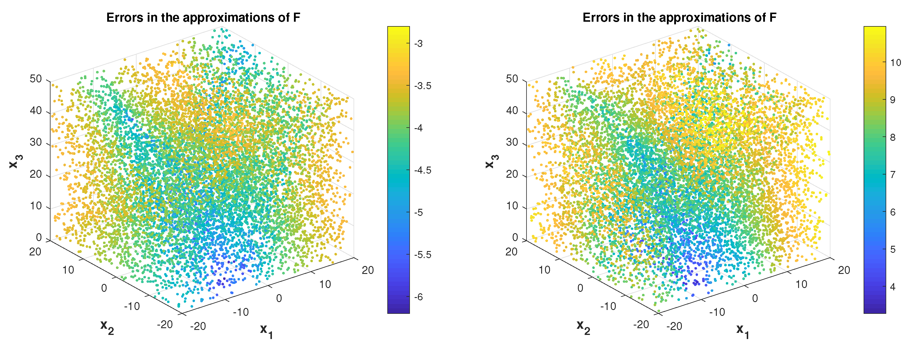
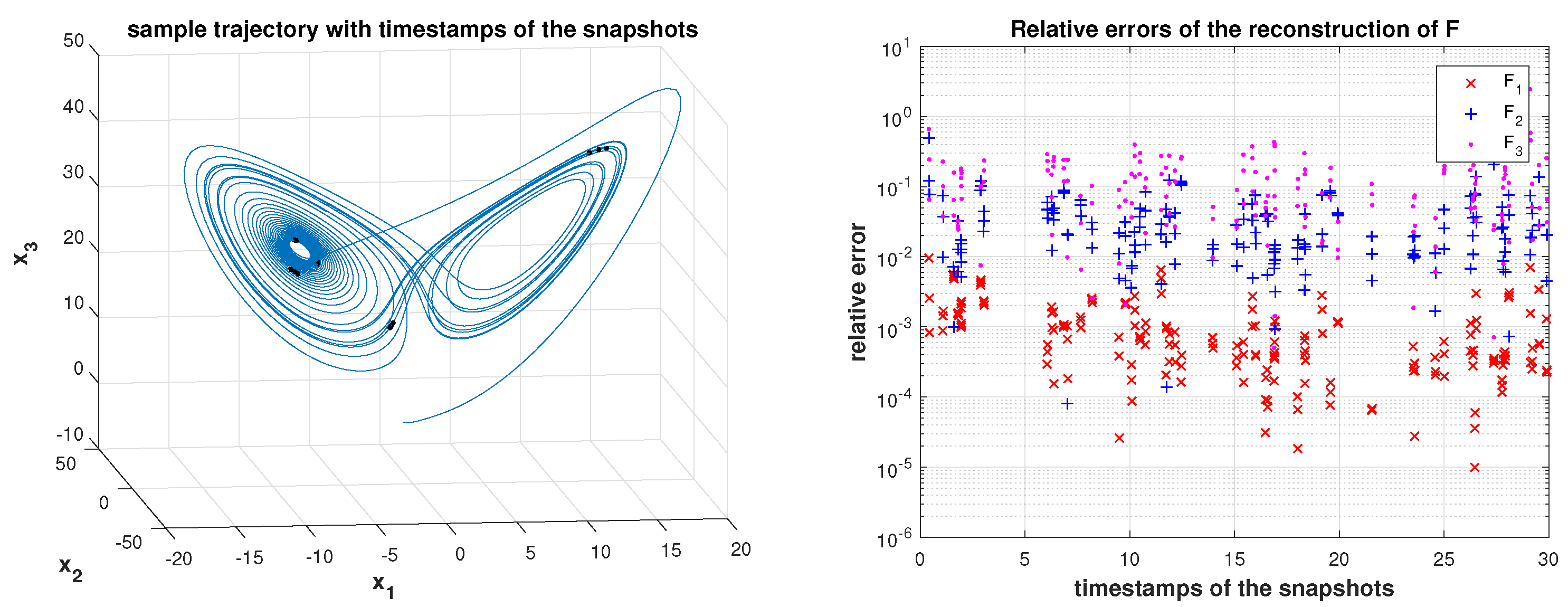
The exact coefficients, ordered to match the grlex ordering of the monomial basis are

$$\begin{array}{rrrrrrrrrrr}\hfill & 1& \hfill x_3& x_2& x_1& x_3^2& x_2{x}_3& x_2^2& x_1{x}_3& x_1{x}_2& x_1^2\\ \hfill F_1:& 0& \hfill 0& \mathbf{1}.\mathbf{0000}\times {\mathbf{10}}^{\mathbf{1}}& -\mathbf{1}.\mathbf{0000}\times {\mathbf{10}}^{\mathbf{1}}& 0& 0& 0& 0& 0& 0\\ \hfill F_2:& 0& \hfill 0& -\mathbf{1}.\mathbf{0000}\times {\mathbf{10}}^{\mathbf{0}}& \mathbf{2}.\mathbf{8000}\times {\mathbf{10}}^{\mathbf{1}}& 0& 0& 0& -\mathbf{1}.\mathbf{0000}\times {\mathbf{10}}^{\mathbf{0}}& 0& 0\\ \hfill F_3:& 0& \hfill -\mathbf{2}.\mathbf{6667}\times {\mathbf{10}}^{\mathbf{0}}& 0& 0& 0& 0& 0& 0& \mathbf{1}.\mathbf{0000}\times {\mathbf{10}}^{\mathbf{0}}& 0\end{array}.$$

To collect data, we ran simulations with 55 random initial conditions and from each trajectory we randomly (independently) selected 55 points, giving a total of $K=3025$ pairs $({\mathbf{x}}_k,{\mathbf{y}}_k)$. The simulations were performed in Matlab, using the ode45() solver in the time interval $[0,0.2]$ with the time step $\delta t={10}^{-3}$. In the key Formula (18), we computed the logarithm in Matlab in two ways, as logm (pinv $\left(O_X\right)\ast O_Y$) and as logm $(O_X\backslash O_Y)$ and obtained nearly the same matrix. Of course, using the pseudoinverse explicitly is not recommended. We will use it in this section for illustrative purposes; recall the discussion in Section 2.2. The computed approximations of the coefficients of (23), with $m=3$, $N=20$ and $m_F=2$, are

$$\begin{array}{rrrrrrrrrrr}\hfill & 1& \hfill x_3& x_2& x_1& x_3^2& x_2{x}_3& x_2^2& x_1{x}_3& x_1{x}_2& x_1^2\\ \hfill F_1:& 3.2\times {10}^{-5}& \hfill -2.5\times {10}^{-6}& \mathbf{1}.\mathbf{0000}\times {\mathbf{10}}^{\mathbf{1}}& -\mathbf{1}.\mathbf{0000}\times {\mathbf{10}}^{\mathbf{1}}& -7.5\times {10}^{-7}& -5.2\times {10}^{-6}& 1.5\times {10}^{-7}& 7.4\times {10}^{-6}& -1.6\times {10}^{-6}& 8.0\times {10}^{-7}\\ \hfill F_2:& -3.4\times {10}^{-5}& \hfill -8.7\times {10}^{-6}& -\mathbf{1}.\mathbf{0000}\times {\mathbf{10}}^{\mathbf{0}}& \mathbf{2}.\mathbf{8000}\times {\mathbf{10}}^{\mathbf{1}}& 4.7\times {10}^{-6}& 1.3\times {10}^{-5}& 8.7\times {10}^{-9}& -\mathbf{1}.\mathbf{0001}\times {\mathbf{10}}^{\mathbf{0}}& -6.1\times {10}^{-6}& 6.1\times {10}^{-6}\\ \hfill F_3:& 2.8\times {10}^{-4}& \hfill -\mathbf{2}.\mathbf{6667}\times {\mathbf{10}}^{\mathbf{0}}& -5.5\times {10}^{-6}& -6.9\times {10}^{-6}& -8.3\times {10}^{-6}& 2.9\times {10}^{-6}& 1.6\times {10}^{-8}& -1.0\times {10}^{-5}& \mathbf{1}.\mathbf{0000}\times {\mathbf{10}}^{\mathbf{0}}& 5.7\times {10}^{-6}\end{array}.$$

The nonzero coefficients are matched to five digits of accuracy, and the remaining coefficients are below $O\left({10}^{-5}\right)$. Nearly the same result is obtained if the samples from all trajectories have the same time stamps. Given the difficulty of the Lorenz example and the fact that the results are obtained by a low dimensional approximation of a nontrivial (numerically simulated) dynamics, the results are good. Analytical properties of the method indicate that increasing dimensions provides increased accuracy, ultimately yielding convergence.

Example 2.

Next, we illustrate the reconstruction of the function $\mathbf{F}$. We simulated the system in the interval $[0,4]$ with $\delta t=0.01$, and used the monomials with the total degree up to $m=3$. In the discrete time grid, we randomly selected 9 positions at which we took three consecutive values from each trajectory; in the second experiment 27 randomly selected values of ${\mathbf{x}}_k$ are taken from each trajectory. The total number of trajectories (with random initial conditions) was set to 150.

$\mathbf{F}$ is approximated using (19). For each ${\mathbf{x}}_k$, we compute the approximation error as

$${ϵ}_k=\underset{i=1,2,3}{max}\frac{|\widetilde{F_i\left({\mathbf{x}}_k\right)}-F_i\left({\mathbf{x}}_k\right)|}{\parallel \mathbf{F}\left({\mathbf{x}}_k\right){\parallel }_{\infty }}.$$

(24)

The sampling points and the values of ${ϵ}_k$ are shown in Figure 1.

Example 3.

Now we use the data snapshots from Example 1, and increase the total degree to $m=9$, thus increasing N from $N=20$ to $N=220$. Recall that $K=3025$. Surprisingly, the computed coefficients are all complex, and are completely off; their absolute values are (the euclidean norms of the real and the imaginary parts of the vector of the computed coefficients are $O\left({10}^6\right)$.

$$\begin{array}{rrrrrrrrrrr}\hfill & 1& \hfill x_3& x_2& x_1& x_3^2& x_2{x}_3& x_2^2& x_1{x}_3& x_1{x}_2& x_1^2\\ \hfill F_1:& 4.6\times {10}^3& \hfill 1.6\times {10}^6& \mathbf{3}.\mathbf{6}\times {\mathbf{10}}^{\mathbf{5}}& \mathbf{3}.\mathbf{0}\times {\mathbf{10}}^{\mathbf{4}}& 1.5\times {10}^4& 1.2\times {10}^4& 4.3\times {10}^3& 1.0\times {10}^4& 9.1\times {10}^3& 1.0\times {10}^4\\ \hfill F_2:& 3.0\times {10}^4& \hfill 1.2\times {10}^6& \mathbf{2}.\mathbf{8}\times {\mathbf{10}}^{\mathbf{5}}& \mathbf{1}.\mathbf{0}\times {\mathbf{10}}^{\mathbf{4}}& 9.6\times {10}^3& 1.2\times {10}^4& 7.6\times {10}^3& \mathbf{2}.\mathbf{1}\times {\mathbf{10}}^{\mathbf{4}}& 9.5\times {10}^3& 5.5\times {10}^3\\ \hfill F_3:& 6.8\times {10}^3& \hfill \mathbf{2}.\mathbf{4}\times {\mathbf{10}}^{\mathbf{5}}& 5.5\times {10}^4& 2.2\times {10}^3& 1.9\times {10}^3& 2.6\times {10}^3& 1.6\times {10}^3& 4.5\times {10}^3& \mathbf{2}.\mathbf{0}\times {\mathbf{10}}^{\mathbf{3}}& 1.1\times {10}^3\end{array}.$$

The approximation of $\mathbf{F}$ is also bad, see Figure 2. Increasing the number of trajectories and samples per trajectory to obtain $K=$ 24,025 did not bring any improvement.

Although increasing N, with correspondingly large K, should be the step toward better approximation, the numerical implementation breaks down. In situation like this one, it is important to find out and understand the sources of the problem.

4.2. What Went Wrong

It is clear that in this computation the most sensitive part is computation of the matrix logarithm, and that this is the most likely source of problems. Indeed, in the last run in Example 3 a warning was issued by the logm() function:

• Warning: the principal matrix logarithm is not defined for A with nonpositive real eigenvalues. A non-principal matrix logarithm is returned.

A closer inspection of the eigenvalues of $U_N$, shown in Figure 3 confirms that $U_N$ indeed has problematic (real negative) eigenvalues.

Although Figure 3 and Figure 4 show numerically computed eigenvalues, by a backward stability analysis argument one can argue that $U_N$ is certainly close to matrices with eigenvalues that preclude computing the logarithm in finite precision arithmetic. Hence, computation of the logarithm must be ill-conditioned as the ill-conditioning is essentially measured as the inverse distance to singularity [27].

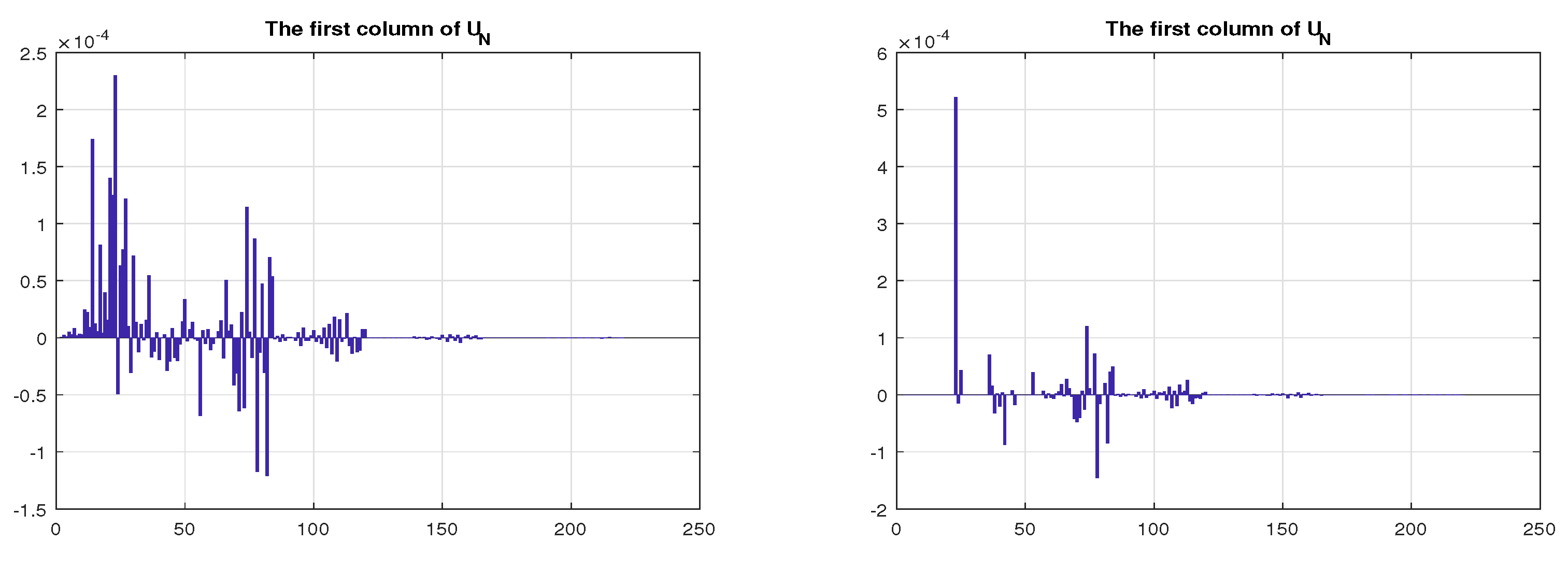
Another look at $U_N$ reveals that its first column is not what it should be. In this example we use monomials and the first basis vector is the constant. Since ${\mathbb{U}}^t{\wp }_1=1·{\wp }_1$, we expect ${\left[{\Phi }_N{\mathbb{U}}_{|{\mathcal{F}}_N}^t\right]}_{\mathcal{B}}{\left[{\wp }_1\right]}_{\mathcal{B}}\equiv U_N{e}_1=e_1=1·{\left[{\wp }_1\right]}_{\mathcal{B}}$, which clearly follows from the solution of the least squares problem (7), if the coefficient matrix is of full column rank. On the other hand, the first column of $U_N$ is computed as shown in Figure 5.

Two conclusions are immediate. First, $O_X$ is considered (by the software) numerically rank deficient. Secondly, two different software solutions of the same problem return two different solutions. For the data shown in Figure 3 and Figure 4, we computed $U_N$ as $\mathtt{pinv}\left(O_X\right)\ast O_Y$. This is in general not a good idea for solving least squares problems; nevertheless, it can be often seen in the literature and software implementations as a textbook-style numerical method for least squares problems, albeit a wrong one. We included it here for instructive purposes. 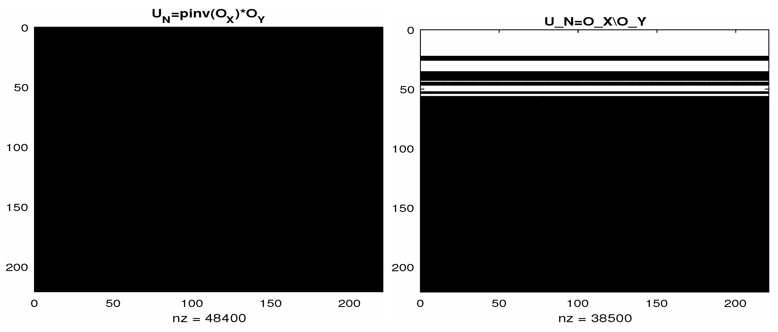If we repeat the experiment with the backslash operator, $O_X\backslash O_Y$, the results are, unfortunately, not better. One conspicuous difference is that, instead of the cluster of absolutely small eigenvalues of $\mathtt{pinv}\left(O_X\right)\ast O_Y$ (see Figure 4), $O_X\backslash O_Y$ has a zero eigenvalue of multiplicity 45. This multiple zero eigenvalue is a consequence of the sparsity structure of $O_X\backslash O_Y$, see Figure 6.

In the course of solving the least squares problem, in both methods (explicit use of the pseudoinverse or the backslash operator), the coefficient matrix $O_X$ is truncated (small singular values are set to zero if $\mathtt{pinv}\left(O_X\right)$ is used; the upper triangular factor is truncated in the case of backslash, which uses a rank revealing QR factorization) and the computed $U_N$, due to rounding errors, is small a perturbation of a rank-deficient matrix with a number of eigenvalues in the vicinity of zero. As a result, the matrix logarithm function fails.

The data shown in Figure 7 are instructive. The condition number of $O_X$ and the distribution of its singular values are nicely revealed by the column norms of $O_X$. The LS solver automatically truncates small singular values that originate from small columns (small basis function values over the snapshots ${\mathbf{x}}_k$) and not necessarily from collinearity in the sense of small angles between basis functions.

Look at the singular values ${\sigma }_1\left(U_N\right)\ge \cdots \ge {\sigma }_N\left(U_N\right)$ in the right panel, in particular the gap ${\sigma }_{176}\left(U_N\right)\approx 1.4058\times {10}^{-6}\gg {\sigma }_{177}\left(U_N\right)\approx 3.9261\times {10}^{-10}$. The numerical rank of $U_N$ is determined as 176 because ${\sigma }_{176}\left(U_N\right)$ is the smallest singular value that is above the threshold $N·\mathtt{eps}·{\sigma }_1\left(U_N\right)\approx 4.6543\times {10}^{-8}$. The index 176 originates in the numerical rank of $O_X$ which is determined in Matlab ($\mathtt{rank}\left(O_X\right)$ returns 176) by the default tolerance. Note that there is no such visible gap (cliff) in the ordered singular values of $O_X$.

Remark 3.

It should be also mentioned here that the cosines of the canonical angles between the ranges of $O_X$ and $O_Y$ are between 0.988 and one (cf. Section 2.1.3), and that we expect the spectrum of $U_N$ not to be too far away from the unit circle. The intuition is that (in the process of computation of $O_X^{†}{O}_Y$) the truncated part of $O_X$ did not (could not) cancel the corresponding part in $O_Y$, which resulted in the problematic cluster of eigenvalues near zero. (In Figure 3, the number of eigenvalues in the cluster around zero is 44, which is the numerical rank deficiency, because the numerical rank is determined (from the singular values) as 176.)

Remark 4.

In the computations pinv $\left(O_X\right)\ast O_Y$ and $O_X\backslash O_Y$, the truncation is conducted based on the SVD and the rank revealing QR factorization, respectively, of $O_X$, independent of $O_Y$. It is more appropriate to solve each LS problem (7) separately (for the corresponding column of $U_N$), and use the truncation strategy following Rust [28]. Note that this is a more general issue because the matrix $O_X^{†}{O}_Y$ is often used in the Koopman/DMD setting. (See [29] for a detailed numerical analysis of the DMD and its variations.) Furthermore, the problem can become even more difficult if we have weighting matrix W with scaling factors that spread over several orders of magnitude. (In this paper, we work with $W={\mathbb{I}}_K$ for the sake of brevity.)

Remark 5.

In the case of noisy data, it might be advantageous to replace the least squares fit with the total least squares ([20], §2.7.6). This is an important issue and we leave it for our future work.

5. Computing ${\left[{\mathit{L}}_{\mathit{N}}\right]}_{\mathcal{B}}$ with Preconditioning

Numerical examples in Section 4 show that implementation of the method in state of the art packages such as Matlab which is straightforward and effortless: the key computation is coded as $\mathtt{logm}(O_X\backslash O_Y)$ or as $\mathtt{logm}(\mathtt{pinv}\left(O_X\right)\ast O_Y)$. However, the results are not always satisfactory, and the problems are both in the computation of $U_N$ (solving the least squares problem) and in computing the matrix logarithm. In this section, we use the structure of the least squares problem solver (reviewed in Section 2.2.1) to introduce a simple modification and then to construct preconditioned computations of $log{U}_N$. These techniques can be combined with the dual method that is analyzed in detail in Section 6 and Section 7.

5.1. A Simple Modification

The first attempt to avoid some of the problems illustrated in Section 4 is to prevent truncation when computing $O_X^{†}{O}_Y$. So we simply run the procedure used in the backslash solver (see Section 2.2.1), but without truncation. More precisely, using the column pivoted QR factorization $O_X\mathsf{\Pi }=QR$, $U_N$ is computed as $U_N=\mathsf{\Pi }{R}^{-1}{Q}^T{O}_Y$.

With $m=9$ and same setting as in Example 1, the computation of the logarithm of $U_N$ was successful. (Matlab function logm() computed a real valued logarithm, without an error/warning message) and the coefficients of (23) are recovered to four digits of accuracy, which is satisfactory. The remaining coefficients are below $O\left({10}^{-4}\right)$ and are discarded in the Formula (19) for reconstructing $\mathbf{F}$. The first column of $U_N$ was $e_1$ up to an error of the order of the roundoff.

The results shown in Figure 8 are encouraging, because they show that the data contain information that can be turned into more accurate output, provided that the algorithm successfully curbs the ill-conditioning. Furthermore, test with $m=10$ (${\kappa }_2\left(U_N\right)\approx 2.9\times {10}^{20}$) showed nearly the same four digit accuracy; with $m=11$ (${\kappa }_2\left(U_N\right)\approx 2.2\times {10}^{24}$) the accuracy dropped to two digits (but the logarithm was successfully computed); with $m=12$ (${\kappa }_2\left(U_N\right)\approx 7.7\times {10}^{26}$) the logarithm is still computed as real matrix, but the accuracy of the computed coefficients drops to $O\left({10}^{-1}\right)$ and the reconstruction of $\mathbf{F}$ fails. However, if we increase K to 24,025 (by sampling more points from more trajectories) the accuracy rebounds to at least for digits both in the coefficients and the reconstruction of $\mathbf{F}$. At $m=16$ ($N=969$ and $K=$ 24,025, or $K=3025$) the accuracy is lost. The condition number of $U_N$ is greater than ${10}^{37}$.

Our adversarial testing is used to expose potential weaknesses of the computational steps in a software implementation of the algorithm. Of course, all these outcomes may vary, depending on the number of trajectories, initial conditions, sampling resolution; in some examples it is possible that the computation of the matrix logarithm breaks down even for smaller values of m. ( Moreover, numerical accuracy, i.e., the conditioning of the problem, heavily depends on the underlying dynamics). In any case, at this point we have to conclude that using the $log{O}_X^{†}{O}_Y$ is a source of nontrivial numerical difficulties that preclude efficient and robust deployment of the Mauroy–Goncalves method. The theoretical convergence (as $N,K\to \infty$, $t\to 0$) is not matched by numerical convergence of a straightforward implementation of the method in finite precision computation.

5.2. Preconditioning the Logarithm of $O_X^{†}{O}_Y$

The discussion in Section 4.2 and Section 5.1 is only one step toward more robust computation—it merely identifies the problem and shows how small changes in an implementation substantially change the final result. Clearly, sufficiently accurate computation of $U_N$ is among the necessary conditions for successful computation of the matrix algorithms. However, this is not sufficient; even if we compute $U_N$ accurately, computation of the logarithm may fail if the matrix is ill-conditioned.

We now introduce a new scheme that uses functional calculus-based preconditioning. If S is any nonsingular matrix, then

$$log\left(O_X^{†}{O}_Y\right)=Slog\left(S^{-1}\left(O_X^{†}{O}_Y\right)S\right)S^{-1}\equiv Slog\left({\left(O_{X}S\right)}^{†}{O}_{Y}S\right)S^{-1}.$$

(25)

Note that replacing $O_X^{†}{O}_Y$ with the similar matrix $S^{-1}\left(O_X^{†}{O}_Y\right)S$ corresponds to changing the basis for matrix representation of the compressed Koopman operator. With the experience from Section 4.2, it is clear that the key is to compute the preconditioned matrix $S^{-1}\left(O_X^{†}{O}_Y\right)S$ without first computing $O_X^{†}{O}_Y$. (Once we compute $O_X^{†}{O}_Y$ explicitly in floating point arithmetic and store it in the machine memory, it may be then too late even for exact computation.)

The conditions on S are:

(i)

Tt should facilitate more accurate computation of the argument $S^{-1}\left(O_X^{†}{O}_Y\right)S={\left(O_{X}S\right)}^{†}{O}_{Y}S$ for the matrix logarithm;

(ii)

It should have preconditioning effect for computing the logarithm of $S^{-1}\left(O_X^{†}{O}_Y\right)S$;

(iii)

The application of S and $S^{-1}$ should be efficient and numerically stable.

Example 4.

To test the concept, we use the same data as in Example 1 with $m=9$, and for the matrix S we take $S=\mathrm{diag}(1/\parallel O_X(:,i){{\parallel }_2)}_{i=1}^N$ and compute

$$L_N=\frac{1}{t}Slog\left({\left(O_{X}S\right)}^{†}\left(O_{Y}S\right)\right)S^{-1}.$$

(26)

Contrary to the failure of the formula $L_N=(1/t)log\left(O_X^{†}{O}_Y\right)$, (26) computes the real logarithm of the explicitly computed ${\left(O_{X}S\right)}^{†}\left(O_{Y}S\right)$, and recovers the coefficients with an $O\left({10}^{-5}\right)$ relative error. That is, we scale $O_X$ and $O_Y$ by $\mathrm{diag}(1/\parallel O_X(:,i){{\parallel }_2)}_{i=1}^N$, and then proceed by solving the least squares problem with the thus scaled matrices. To understand the positive result, we first note that the condition number of $O_{X}S$ is ${\kappa }_2\left(O_{X}S\right)\approx 1.3\times {10}^9$, so the least squares solution is computed without truncation. The condition number of ${\left(O_{X}S\right)}^{†}\left(O_{Y}S\right)$ was ${\kappa }_2\left({\left(O_{X}S\right)}^{†}\left(O_{Y}S\right)\right)\approx 6.4\times {10}^5$. (The condition number of $O_X^{†}{O}_Y$ is $O\left({10}^{20}\right)$ so that the matrix is considered numerically rank deficient.) With $m=12$ we had $\kappa \left(U_N\right)\approx 6.9\times {10}^{61}$ and ${\kappa }_2\left({\left(O_{X}S\right)}^{†}\left(O_{Y}S\right)\right)\approx 1.4\times {10}^{13}$; the coefficients are recovered to three accurate digits and approximation of $\mathbf{F}$ is with error slightly larger than the one in the right panel of Figure 8.

However, as m increases, the diagonal scaling cannot cope with the increased condition number; already at $m=15$, a complex non-principal value of the logarithm is computed, with some eigenvalues whose imaginary parts are equal $\pi /\delta t$. The computed $U_N$ has a cluster of eigenvalues around zero. For the record, ${\kappa }_2\left(U_N\right)\approx 2.2\times {10}^{220}$, ${\kappa }_2\left({\left(O_{X}S\right)}^{†}\left(O_{Y}S\right)\right)\approx 6.7\times {10}^{78}$. Surprisingly, the approximate coefficients, although complex, have small imaginary parts (of the order of the roundoff) and their real parts still provide reasonably good approximations of the true coefficients.

5.2.1. Scaled QR Factorization Based Preconditioner

To develop a stronger preconditioner, we start with the following observation: No matter how ill-conditioned $O_X$ and $O_Y$ may be (in the sense of badly scaled columns), the distance between the ranges of $O_X$ and $O_Y$, as measured by the canonical angles between the subspaces, should not be too big. (Intuitively, $O_Y$ contains the observables evaluated at the states ${\mathbf{y}}_k$ downstream in time $\delta t$ from the ${\mathbf{x}}_k$’s used in $O_X$. Recall Remark 3.)

Hence, if we compute the QR factorization of $O_X$, the inverse of its triangular factor will have a preconditioning effect on $O_Y$ by postmultiplication. This leads to Algorithm 1.

Algorithm 1  $\left[L_N\right]=\mathrm{Inf}\_\mathrm{Generator}\_\mathrm{QRSC}(O_X,O_Y,T)$

Input:  $O_X\in {\mathbb{C}}^{K\times N}$, $O_Y\in {\mathbb{C}}^{K\times N}$, $T>0$   1: $S=\mathrm{diag}(1/\parallel O_X(:,i){{\parallel }_2)}_{i=1}^N$   2: $[Q_X,{\widehat{R}}_X]=\mathrm{qr}\left(O_{X}S\right)${QR factorization}   3: ${\widehat{U}}_N=Q_X^T\left(O_{Y}S\right){\widehat{R}}_X^{-1}$ {${\widehat{U}}_N$ is similar to $O_X^{†}{O}_Y$.}   4: ${\widehat{L}}_N=log\left({\widehat{U}}_N\right)$   5: $L_N=(1/T)S\left({\widehat{R}}_X^{-1}{\widehat{L}}_N{\widehat{R}}_X\right)S^{-1}$ Output:  $L_N$. {$L_N=(1/T)log\left(O_X^{†}{O}_Y\right)$}

Example 5.

To test this algorithm, we use the data from Example 1, take $m=15$ and increase the number of snapshots to K = 24,025. The matrix ${\widehat{U}}_N$ is well conditioned, ${\kappa }_2\left({\widehat{U}}_N\right)\approx 1.2\times {10}^2$, and computing the matrix logarithm is successful. The coefficients are recovered to four digits of accuracy, and the reconstruction of $\mathbf{F}$ is slightly better than the one shown in the right panel in Figure 8.

This example, as a test of the proposed approach, is encouraging. Our next task is to further develop the method along the lines of Algorithm 1, and to provide a robust method with accompanying numerical analysis, and finally to implement it as a reliable software toolbox.

5.2.2. Pivoted QR Factorization Based Preconditioner

Since in this approach the matrix logarithm is the most critical and numerically most difficult computational task, the preprocessing/preconditioning aims to ensure successful completion of that particular step in the method. The back application of the similarity is also an important step. In Algorithm 1, the main preconditioning is performed by an upper triangular factor from the QR factorization, and by its inverse. For a numerically robust computation, it is important that the QR factorization is computed accurately even in the case of wildly scaled data, and, moreover, that the resulting triangular factor is rank revealing and well structured. These goals can be accomplished by pivoting. In this subsection we outline the main principles along which the idea of QR factorization-based preconditioned computation of the matrix $L_N$ (matrix representation of a compression of the infinitesimal generator) can be further pursued.

The column pivoting has the rank revealing property and the triangular factor is diagonally dominant in a very strong sense, see e.g., [23,30] and (13).

In the case of Businger–Golub pivoting, we know that $R_X={\mathsf{\Delta }}_X{T}_X$, where ${\mathsf{\Delta }}_X=\mathrm{diag}\left(\right|{\left(R_X\right)}_{ii}{\left|\right)}_{i=1}^N$ and $T_X$ is well conditioned. Hence, $R_X^{-1}=T_X^{-1}{\mathsf{\Delta }}_X^{-1}$, and after Line 3 in Algorithm 2 one can insert another preconditioning with ${\mathsf{\Delta }}_X$. We omit the details for the sake of brevity. Instead, we conclude this theme with few remarks that should be useful for further study and implementation.

Algorithm 2  $\left[L_N\right]=\mathrm{Inf}\_\mathrm{Generator}\_\mathrm{QRCP}(O_X,O_Y,T)$

Input:  $O_X\in {\mathbb{C}}^{K\times N}$, $O_Y\in {\mathbb{C}}^{K\times N}$, $T>0$   1: Reorder the snapshots by simultaneous row permutation of $O_X$ and $O_Y$; see Remark 6.   2: $[Q_X,R_X,{\mathsf{\Pi }}_X]=\mathrm{qr}\left(O_X\right)${Rank revealing QR factorization with column pivoting}   3: ${\widehat{U}}_N=Q_X^T\left(O_Y{\mathsf{\Pi }}_X\right)R_X^{-1}$ {${\widehat{U}}_N$ is similar to $O_X^{†}{O}_Y$.}   4: ${\widehat{L}}_N=log\left({\widehat{U}}_N\right)$   5: $L_N=(1/T){\mathsf{\Pi }}_X\left(R_X^{-1}{\widehat{L}}_N{R}_X\right){\mathsf{\Pi }}_X^T$ Output:  $L_N$. {$L_N=(1/T)log\left(O_X^{†}{O}_Y\right)$}

Remark 6.

For the numerical accuracy of the QR factorization, an additional row pivoting may be needed to obtain that the rows are ordered so that their ${\ell }_{\infty }$ norms are decreasing, see [31,32]. If Ψ is a permutation matrix that encodes the row pivoting, then ${(\Psi O_X)}^{†}=O_X^{†}{\Psi }^T$, so that ${(\Psi O_X)}^{†}(\Psi O_Y)=O_X^{†}{O}_Y$. This means that using the additional row pivoting in the QR factorization in Algorithm 2 is equivalent to a particular ordering of the data snapshots. The column pivoting corresponds to reordering the basis’ functions. Both reorders of the data are allowed operations and can thus be used to enhance numerical robustness of the computation.

Remark 7.

If $K\gg 2N$ then it pays off to change the coordinates by computing the QR factorization

$$\left(\begin{array}{cc}{Q}_X& Q_Y\end{array}\right)=\mathcal{Q}\left(\begin{array}{c}\mathcal{R}\\ \mathbf{0}\end{array}\right),$$

and use the corresponding columns of $\mathcal{R}$ instead of $O_X$ and $O_Y$. This follows the idea of the QR-compressed DMD [29].

Remark 8.

The key assumption in the above described method is that $K\gg N$, i.e., that both $O_X$ and $O_Y$ are tall matrices; their columns are in a high dimensional space and with suitable transformation S in the column spaces ($O_X\mapsto O_{X}S$, $O_Y\mapsto O_{Y}S$) we can improve the condition numbers. By the (variational) monotonicity principle, supplying more snapshots (increasing K) moves the singular values of $O_X$ and $O_Y$ to the right, thus improving the condition numbers of both matrices. Since, by the underlying continuity, the canonical angles between the ranges of $O_X$ and $O_Y$ are expected to be away from $\pi /2$, and $U_N=O_X^{†}{O}_Y$ is going to be nonsingular. Moreover, the overall condition number of the computation can be controlled using our proposed modifications that are designed to ensure stable computation of the matrix logarithm.

6. Dual Method

It is clear that the values of N linearly independent functions ${\wp }_1,\dots ,{\wp }_N$ over the discrete set ${\mathbf{x}}_1,\dots ,{\mathbf{x}}_K$ of $K<N$ snapshots (that is, with only the tabulated values in the $K\times N$ matrices $O_X$, $O_Y$) contain redundancy. On the other hand, increasing the space dimension N is a way to lift the data to higher dimensional space; more observables improve both the DMD and KMD analyses. Note that, in the case $N>K$, both the compression $U_N={\left[{\Phi }_N{\mathbb{U}}_{|{\mathcal{F}}_N}^t\right]}_{\mathcal{B}}=O_X^{†}{O}_Y$ and the EDMD matrix ($U_N^T$) are rank deficient; unfortunately, the infinitesimal generator identification framework cannot work in that setting because the matrix logarithm is not defined. It should be stressed here that, e.g., in the DMD setting, the action of the operator given by the data is restricted to an at most K-dimensional subspace in the N dimensional space, and that the approximations of the Koopman modes are obtained by a Rayleigh–Ritz extraction. Hence, any operator (matrix) function of $U_N$ only makes sense and has a practical usability in the context of an approximation from the subspace defined by the data.

In [8], a dual method is proposed, which instead of $U_N=O_X^{†}{O}_Y$ works with the logarithm of $U_K=O_Y{O}_X^{†}$. In this section we first provide, in Section 6.1, a detailed linear algebra description of the dual method that will facilitate a more general formulation that allows for modifications which may lead to better numerical algorithms. In fact, we show in Section 7 that the dual method of [8] is but a special case of subspace projection methods, and we show how to exploit this for design of numerically better schemes.

6.1. A Rayleigh Quotient Formulation

In the dual formulation, the transition from $U_N$ to $U_K$ can be formulated as another compression of ${\mathbb{U}}^t$ onto a particular K-dimensional subspace of ${\mathcal{F}}_N$.

Proposition 3.

If we define $\left(\begin{array}{ccc}{\mathit{\psi }}_1\left(x\right)& \dots & {\mathit{\psi }}_K\left(x\right)\end{array}\right)=\left(\begin{array}{ccc}{\wp }_1\left(x\right)& \dots & {\wp }_N\left(x\right)\end{array}\right)O_X^{†}$, then (assuming $O_X$ is of full row rank K), ${\mathcal{B}}_K=\{{\mathit{\psi }}_1,\dots ,{\mathit{\psi }}_K\}$ is a basis of the K dimensional subspace ${\mathcal{F}}_K\subset {\mathcal{F}}_N$, and $U_K=O_Y{O}_X^{†}$ is the matrix representation of the Rayleigh quotient ${\Phi }_K{\mathbb{U}}_{|{\mathcal{F}}_K}^t$ in which ${\Phi }_K:\mathcal{F}\to {\mathcal{F}}_K$ is the least squares projection as in Section 2.1.1. The matrix $U_K$ is the matrix Rayleigh quotient of $U_N$ with respect to the range of $O_X^{†}$, i.e., $U_K=O_X{U}_N{O}_X^{†}$ and $U_N{O}_X^{†}=O_X^{†}{U}_K$. Furthermore, the Rayleigh quotient with respect to $O_X^{†}$ is the same for all matrices from the set $\mathcal{N}$ (see (10)):

$$O_X(O_X^{†}{O}_Y+{\Psi }_0\Xi )O_X^{†}=O_Y{O}_X^{†}.(Note here that{\left(O_X^{†}\right)}^{†}=O_X.)$$

(27)

Proof. 

First, note that the basis functions ${\mathit{\psi }}_1,\dots ,{\mathit{\psi }}_K$ evaluated at ${\mathbf{x}}_1,\dots ,{\mathbf{x}}_K$ can be tabulated as the matrix

$$O_{X,K}=\left(\begin{array}{cccc}{\mathit{\psi }}_1\left({\mathbf{x}}_1\right)& {\mathit{\psi }}_2\left({\mathbf{x}}_1\right)& \dots & {\mathit{\psi }}_K\left({\mathbf{x}}_1\right)\\ ⋮& ⋮& \dots & ⋮\\ {\mathit{\psi }}_1\left({\mathbf{x}}_K\right)& {\mathit{\psi }}_2\left({\mathbf{x}}_K\right)& \dots & {\mathit{\psi }}_K\left({\mathbf{x}}_K\right)\end{array}\right)=O_X{O}_X^{†}={\mathbb{I}}_K,$$

and that for a $g\in {\mathcal{F}}_K$, its representation in the basis ${\mathcal{B}}_K$ is ${\left[g\right]}_{{\mathcal{B}}_K}={\left(\begin{array}{c}g\left({\mathbf{x}}_1\right),\dots ,g\left({\mathbf{x}}_K\right)\end{array}\right)}^T$; see (6), where we take $W=\mathbb{I}$ for the sake of simplicity. Similarly, $({\mathbb{U}}^t{\mathit{\psi }}_1,\dots ,{\mathbb{U}}^t{\mathit{\psi }}_K)$ evaluated at ${\mathbf{x}}_1,\dots ,{\mathbf{x}}_K$ yields the matrix $O_{Y,K}=O_Y{O}_X^{†}$. Now, as in Section 2.1.2, $U_K=O_{X,K}^{†}{O}_{Y,K}=O_Y{O}_X^{†}$. Relation (27) is easily checked. □

If $U_K$ is nonsingular then the identification scheme should be recast in terms of $log{U}_K$. In the basis ${\mathcal{B}}_K$ we have then the following representations of the Rayleigh quotient ${\Phi }_K{\mathbb{U}}_{|{\mathcal{F}}_K}^t$ and its logarithm.

Corollary 1.

The matrix representations of the compressed ${\mathbb{U}}^t$ and its logarithm (if defined) are as follows: For any ${({\mathsf{g}}_1,\dots ,{\mathsf{g}}_K)}^T\in {\mathbb{C}}^K$,

$$\begin{array}{ccc}\hfill {\Phi }_K{\mathbb{U}}_{|{\mathcal{F}}_K}^t((\begin{array}{ccc}{\mathit{\psi }}_1(x)& \dots & {\mathit{\psi }}_K(x)\end{array})(\begin{array}{c}{\mathsf{g}}_1\\ ⋮\\ {\mathsf{g}}_K\end{array}))& =& (\begin{array}{ccc}{\mathit{\psi }}_1(x)& \dots & {\mathit{\psi }}_K(x)\end{array})(U_K(\begin{array}{c}{\mathsf{g}}_1\\ ⋮\\ {\mathsf{g}}_K\end{array})),\hfill \\ \hfill log({\Phi }_K{\mathbb{U}}_{|{\mathcal{F}}_K}^t)((\begin{array}{ccc}{\mathit{\psi }}_1(x)& \dots & {\mathit{\psi }}_K(x)\end{array})(\begin{array}{c}{\mathsf{g}}_1\\ ⋮\\ {\mathsf{g}}_K\end{array}))& =& (\begin{array}{ccc}{\mathit{\psi }}_1(x)& \dots & {\mathit{\psi }}_K(x)\end{array})(log\left(U_K\right)(\begin{array}{c}{\mathsf{g}}_1\\ ⋮\\ {\mathsf{g}}_K\end{array})).\hfill \end{array}$$

Next, we consider function evaluation at ${\mathbf{y}}_k={\phi }^t\left({\mathbf{x}}_k\right)$, $k=1,\dots ,K$.

Proposition 4.

Let $f={\sum }_{i=1}^N{\mathsf{f}}_i{\wp }_i\in {\mathcal{F}}_N$. Then

$$\left(\begin{array}{c}{\mathbb{U}}^{t}f\left({\mathbf{x}}_1\right)\\ ⋮\\ {\mathbb{U}}^{t}f\left({\mathbf{x}}_K\right)\end{array}\right)=\left(\begin{array}{c}f\left({\mathbf{y}}_1\right)\\ ⋮\\ f\left({\mathbf{y}}_K\right)\end{array}\right)=O_Y{O}_X^{†}\left(\begin{array}{c}f\left({\mathbf{x}}_1\right)\\ ⋮\\ f\left({\mathbf{x}}_K\right)\end{array}\right)+O_Y({\mathbb{I}}_N-O_X^{†}{O}_X)\left(\begin{array}{c}{\mathsf{f}}_1\\ ⋮\\ {\mathsf{f}}_N\end{array}\right).$$

(28)

If ${\mathbb{I}}_N\ne O_X^{†}{O}_X$, then the second term on the right hand side in (28) is zero if and only if the ${\mathsf{f}}_i$’s are of the form ${\left(\begin{array}{c}{\mathsf{f}}_i\end{array}\right)}_{i=1}^N=O_X^{†}{\left(\begin{array}{c}{\mathsf{g}}_k\end{array}\right)}_{k=1}^K$ with arbitrary ${\mathsf{g}}_k$’s. Furthermore, if $g={\sum }_{i=1}^K{\mathsf{g}}_i{\mathit{\psi }}_i\in {\mathcal{F}}_K\subset {\mathcal{F}}_N$, then ${\mathsf{g}}_i=g\left({\mathbf{x}}_i\right)$ and

$$\left(\begin{array}{c}{\mathbb{U}}^{t}g\left({\mathbf{x}}_1\right)\\ ⋮\\ {\mathbb{U}}^{t}g\left({\mathbf{x}}_K\right)\end{array}\right)=O_Y{O}_X^{†}\left(\begin{array}{c}g\left({\mathbf{x}}_1\right)\\ ⋮\\ g\left({\mathbf{x}}_K\right)\end{array}\right),\left(\begin{array}{c}log\left({\Phi }_K{\mathbb{U}}_{|{\mathcal{F}}_K}^t\right)g\left({\mathbf{x}}_1\right)\\ ⋮\\ log\left({\Phi }_K{\mathbb{U}}_{|{\mathcal{F}}_K}^t\right)g\left({\mathbf{x}}_K\right)\end{array}\right)=log\left(O_Y{O}_X^{†}\right)\left(\begin{array}{c}g\left({\mathbf{x}}_1\right)\\ ⋮\\ g\left({\mathbf{x}}_K\right)\end{array}\right).$$

(29)

Proof. 

For (28), it suffices to write

$$\left(\begin{array}{c}f\left({\mathbf{y}}_1\right)\\ ⋮\\ f\left({\mathbf{y}}_K\right)\end{array}\right)=O_Y\left(\begin{array}{c}{\mathsf{f}}_1\\ ⋮\\ {\mathsf{f}}_N\end{array}\right)=O_Y(O_X^{†}{O}_X+{\mathbb{I}}_N-O_X^{†}{O}_X)\left(\begin{array}{c}{\mathsf{f}}_1\\ ⋮\\ {\mathsf{f}}_N\end{array}\right).$$

For the first relation in (29), note that $g={\sum }_{i=1}^K{\mathsf{g}}_i{\mathit{\psi }}_i$ evaluated at ${\mathbf{y}}_1,\dots ,{\mathbf{y}}_K$ reads

$$\left(\begin{array}{c}g\left({\mathbf{y}}_1\right)\\ ⋮\\ g\left({\mathbf{y}}_K\right)\end{array}\right)=O_Y{O}_X^{†}\left(\begin{array}{c}{\mathsf{g}}_1\\ ⋮\\ {\mathsf{g}}_K\end{array}\right),\mathrm{where}{\mathsf{g}}_i=g\left({\mathbf{x}}_i\right)\mathrm{because} O_{X,K}={\mathbb{I}}_K.$$

 □

Hence, using the last relation and $\mathbb{L}=\mathbf{F}·\nabla \approx (1/t)log\left({\Phi }_K{\mathbb{U}}_{|{\mathcal{F}}_K}^t\right)$ in ${\mathcal{F}}_K$ (evaluated at the snapshots ${\mathbf{x}}_i$), we have

$$\left(\begin{array}{c}\mathbf{F}·\nabla g\left({\mathbf{x}}_1\right)\\ ⋮\\ \mathbf{F}·\nabla g\left({\mathbf{x}}_K\right)\end{array}\right)\approx \frac{1}{t}log\left(O_Y{O}_X^{†}\right)\left(\begin{array}{c}g\left({\mathbf{x}}_1\right)\\ ⋮\\ g\left({\mathbf{x}}_K\right)\end{array}\right).$$

(30)

If we choose $g\left(\mathbf{x}\right)=x_j$, $j=1,\dots ,n$, respectively, (where $\mathbf{x}={(x_1,\dots ,x_n)}^T$) then $\mathbf{F}·\nabla g\left(\mathbf{x}\right)=F_j\left(\mathbf{x}\right)$ and we obtain approximate filed values $\widetilde{\mathbf{F}\left({\mathbf{x}}_i\right)}$ defined as

$$\left(\begin{array}{c}{\widetilde{\mathbf{F}\left({\mathbf{x}}_1\right)}}^T\\ ⋮\\ {\widetilde{\mathbf{F}\left({\mathbf{x}}_K\right)}}^T\end{array}\right)=\frac{1}{t}log\left(O_Y{O}_X^{†}\right)\left(\begin{array}{c}{\mathbf{x}}_1^T\\ ⋮\\ {\mathbf{x}}_K^T\end{array}\right).$$

(31)

Note however that (30), (31) require that $g\in {\mathcal{F}}_K$. Furthermore, the approximations of $\mathbf{F}$ are given only at the sequence ${\mathbf{x}}_1,\dots ,{\mathbf{x}}_K$.

Global Identification of $\mathbf{F}$

After identifying the values $\mathbf{F}\left({\mathbf{x}}_k\right)$, the idea is to use the ansatz

$$\mathbf{F}\left(x\right)=\left(\begin{array}{c}{F}_1\left(x\right)\\ ⋮\\ F_n\left(x\right)\end{array}\right),F_j\left(x\right)=\sum _{k=1}^{N_F}{\phi }_{kj}{h}_j\left(x\right),$$

(32)

where $h_1,\dots ,h_{N_F}$ are chosen from a dictionary of functions, possibly different from the basis used to lift the data and identify the compression of the infinitesimal generator. Then we obtain the sequence of least squares problems

$${\parallel \left(\begin{array}{ccc}{h}_1\left({\mathbf{x}}_1\right)& \dots & h_{N_F}\left({\mathbf{x}}_1\right)\\ h_1\left({\mathbf{x}}_2\right)& \dots & h_{N_F}\left({\mathbf{x}}_2\right)\\ ⋮& \dots & ⋮\\ h_1\left({\mathbf{x}}_K\right)& \dots & h_{N_F}\left({\mathbf{x}}_K\right)\end{array}\right)\left(\begin{array}{c}{\phi }_{1j}\\ {\phi }_{2j}\\ ⋮\\ {\phi }_{N_{F}j}\end{array}\right)-\left(\begin{array}{c}{\tilde{F}}_j\left({\mathbf{x}}_1\right)\\ {\tilde{F}}_j\left({\mathbf{x}}_2\right)\\ ⋮\\ {\tilde{F}}_j\left({\mathbf{x}}_K\right)\end{array}\right)\parallel }_2^2⟶\underset{{\phi }_{1j}\dots {\phi }_{N_{F}j}}{min},j=1,\dots ,n,$$

(33)

that can also be equipped with a regularization factor that promotes sparse solution.

6.2. A Numerical Example

As in Section 4, a simple but difficult example can be used to explore the numerical feasibility of the derived scheme. It has been shown in [8] that the method works well for the Lorenz system on small time intervals. In the following example, we increase the time domain and test the accuracy of the reconstruction of $\mathbf{F}$. An ill-conditioned problem is obtained by taking the total degree of the polynomials to be 12. Although this may seem artificial, it is useful because it provides numerically difficult cases that expose the weaknesses of the computational scheme and excellent case studies for better understanding and further development.

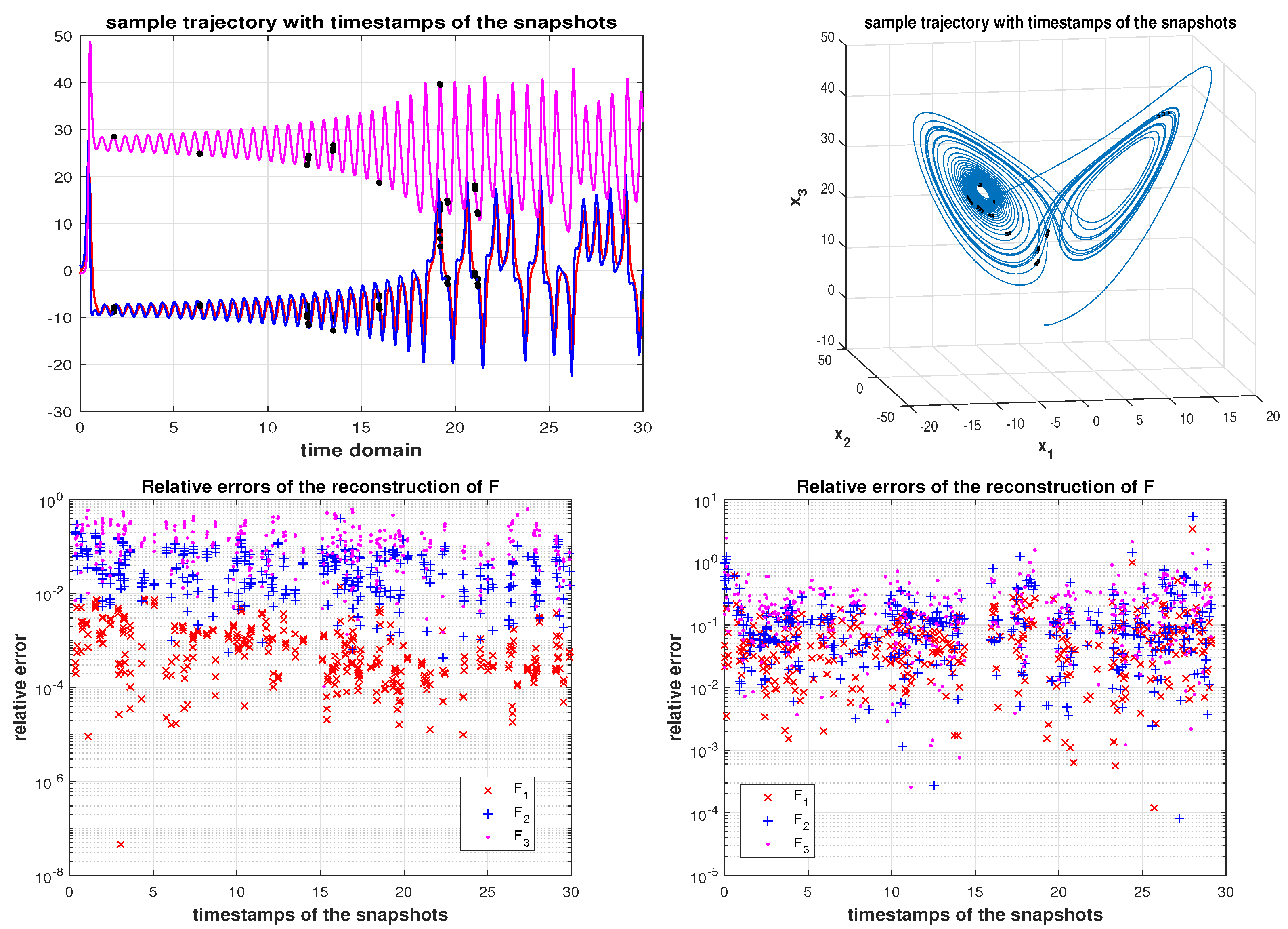
Example 6.

In this example we run simulation of the Lorenz system with time resolution $\delta t={10}^{-3}$ on the intervals $[0,0.1]$, $[0,0.18]$ and $[0,0.19]$. The basis functions ${\wp }_i$ are the monomials with total degree up to $m=12$. We generate 12 trajectories with random initial conditions, and from each trajectory we sample three consecutive snapshots at ten randomly selected positions; the matrices $O_X$, $O_Y$ are thus $360\times 455$. In the reconstruction Formula (31), the matrix logarithm is computed in Matlab as logm(OY/OX); in all three runs, logm() issued a warning that a non-principal value of the algorithm was computed. The reconstruction error is measured component-wise and snapshot-wise as

$${ϵ}_k^{\left(i\right)}=\frac{|\widetilde{F_i\left({\mathbf{x}}_k\right)}-F_i\left({\mathbf{x}}_k\right)|}{\parallel \mathbf{F}\left({\mathbf{x}}_k\right){\parallel }_{\infty }},i=1,\dots n;k=1,\dots ,K.$$

(34)

In addition, we measure the total error of the tabulated values in the Frobenius norm as

$$\tau =\parallel {\left(\widetilde{F_i\left({\mathbf{x}}_k\right)}\right)}_{k,i=1}^{K,n}-{\left(F_i\left({\mathbf{x}}_k\right)\right)}_{k,i=1}^{K,N}{\parallel }_F/{\parallel {\left(F_i\left({\mathbf{x}}_k\right)\right)}_{k,i=1}^{K,N}\parallel }_F.$$

(35)

In Figure 9, we show the errors ${ϵ}_k^{\left(i\right)}$ for the intervals $[0,0.1]$ and $[0,0.18]$; in the case of the time interval $[0,0.19]$, the method broke down and the reconstructed values were computed as NaN’s.

The results depend on the initial conditions used to generate sample trajectories. In the above experiments, each initial condition is taken as a normally distributed $3\times 1$ vector generated in Matlab using randn. If we generate the initial conditions as uniformly distributed inside the sphere of radius $0.1$, centered at the origin, then for all three test intervals the error τ was $O\left({10}^{-3}\right)$. With such initialization, the same level of accuracy is then maintained for larger time intervals, up to $[0,0.4]$; for $[0,0.41]$ the error increased to $\tau \approx 0.1$ and for $[0,0.42]$ the result was NaN.

This example shows that numerical (software) implementation of the dual method requires additional analysis and modifications, similar to the main method. In the next section we explore numerical linear algebra techniques that could facilitate a more robust implementation.

7. Subspace Selection

The approximation (31) is based on a particular K-dimensional subspace of ${\mathcal{F}}_N=\mathrm{span}({\wp }_1,\dots ,{\wp }_N)$, where (in the case of monomial basis) the choice of the new basis functions precludes direct coefficient comparisons with (17), (19). Instead, the identification procedure follows the lines of (30)–(33).

We can set up a more general framework: independent of the ratio $N/K$ (and independent of the formulation—original or dual) we can seek other suitable subspaces of ${\mathcal{F}}_N$, and not necessarily of dimension K. The selection criterion is numerical: both the subspace and its dimension $\widehat{N}$ should be determined with respect to the numerical conditioning of the matrix representations at the finite sequence ${\mathbf{x}}_1,\dots ,{\mathbf{x}}_K$. A basis of such a $\widehat{N}$-dimensional subspace ${\mathcal{F}}_{\widehat{N}}$ of ${\mathcal{F}}_N$ is written as $({\mathit{\psi }}_1,\dots ,{\mathit{\psi }}_{\widehat{N}})=({\wp }_1,\dots ,{\wp }_N)\mathcal{S}$, where $\mathcal{S}$ is $N\times \widehat{N}$ selection operator, i.e., matrix, of rank $\widehat{N}$. The tabulated values of $({\mathit{\psi }}_1,\dots ,{\mathit{\psi }}_{\widehat{N}})$ at ${\mathbf{x}}_1,\dots ,{\mathbf{x}}_K$ are easily computed as $O_{X,\mathcal{S}}=O_X\mathcal{S}$. Similarly, the tabulated values of $({\mathbb{U}}^t{\mathit{\psi }}_1,\dots ,{\mathbb{U}}^t{\mathit{\psi }}_{\widehat{N}})$ are $O_{Y,\mathcal{S}}=O_Y\mathcal{S}$.

Certainly, $\widehat{N}\le min(K,N)$. If e.g., $K<N$, we aim at $\widehat{N}=K$, but we will have option that a numerical algorithm decides whether that choice is feasible, depending on the level of ill-conditioning.

The subspace selection operator $\mathcal{S}$ should ensure that, if needed, the constructed basis of ${\mathcal{F}}_{\widehat{N}}$ contains $\ell <\widehat{N}$ a priori selected functions ${\wp }_{i_1},\dots ,{\wp }_{i_{\ell }}$ (recall the identification procedure outlined in Section 3.2) and that $O_{X,\mathcal{S}}$ is well conditioned. This implicitly restricts ℓ to be at most K, and in practice $\ell \ll K$. Furthermore, the remaining $\widehat{N}-\ell$ basis functions should be selected among the ${\wp }_j$’s. In other words, we seek $\mathcal{S}$ as a selection of $\widehat{N}$ columns of the identity ${\mathbb{I}}_N$. This is achieved by the following two step procedure:

• (Optional) Define ${\mathcal{S}}_0$ as the $N\times N$ permutation matrix that moves the selected functions to the leading positions, i.e., such that $({\wp }_1,\dots ,{\wp }_N){\mathcal{S}}_0=({\wp }_{i_1},\dots ,{\wp }_{i_{\ell }},\dots )$.
• Add to these ℓ functions a selection of $\widehat{N}-\ell$ functions that are most linearly independent in the orthogonal complement of $\mathrm{span}({\wp }_{i_1},\dots ,{\wp }_{i_{\ell }})$ as seen on the discrete points ${\mathbf{x}}_1,\dots ,{\mathbf{x}}_K$.

The second step, which can be designated as basis pruning, is based on the numerical rank revealing techniques.

7.1. Pruning the Basis $({\wp }_1,\dots ,{\wp }_N)$

Removing the basis functions ${\wp }_j$ that carry numerically redundant information on the set ${\mathbf{x}}_1,\dots ,{\mathbf{x}}_K$ can be automated using the rank revealing QR factorization [23] as follows. First, compute the QR factorization of the selected functions, with an optional column pivoting

$$\left(O_X{\mathcal{S}}_0\right)(:,1:\ell ){\mathsf{\Pi }}_1=Q_1\left(\begin{array}{c}{R}_{11}\\ \mathbf{0}\end{array}\right)=\left(\begin{array}{ccccc}.& .& .& .& .\\ .& .& .& .& .\\ .& .& .& .& .\\ .& .& .& .& .\\ .& .& .& .& .\end{array}\right)\left(\begin{array}{cc}*& *\\ 0& *\\ 0& 0\\ 0& 0\\ 0& 0\end{array}\right),$$

(36)

and then apply $Q_1^{*}$ to the remaining $N-\ell$ columns to obtain

$$Q_1^{*}{O}_X{\mathcal{S}}_0({\mathsf{\Pi }}_1\oplus {\mathbb{I}}_{N-\ell })=\left(\begin{array}{cc}{R}_{11}& {\tilde{R}}_{12}\\ \mathbf{0}& {\tilde{R}}_{22}\end{array}\right)=\left(\begin{array}{cccccccc}*& *& \times & \times & \times & \times & \times & \times \\ 0& *& \times & \times & \times & \times & \times & \times \\ 0& 0& +& +& +& +& +& +\\ 0& 0& +& +& +& +& +& +\\ 0& 0& +& +& +& +& +& +\end{array}\right).$$

(37)

(The structure of the computed matrices is illustrated in (36), (37) for $K=5$, $N=8$, $\ell =2$.) Now, the columns of ${\tilde{R}}_{22}$ are the coordinates of the projection of the trailing $N-\ell$ columns of $O_X{\mathcal{S}}_0$ onto the $K-\ell$ dimensional orthogonal complement of the span of the leading ℓ columns (of $O_X{\mathcal{S}}_0$, at this moment assumed linearly independent). A well conditioned selection of $\widehat{N}-\ell$ columns can be computed by another column pivoted (rank revealing) QR factorization

$${\tilde{R}}_{22}{\mathsf{\Pi }}_2=\left(\begin{array}{cccccc}+& +& +& +& +& +\\ +& +& +& +& +& +\\ +& +& +& +& +& +\end{array}\right){\mathsf{\Pi }}_2=Q_2(\begin{array}{cc}{R}_{22}& R_{23}\end{array})=Q_2\left(\begin{array}{cccccc}🟉& 🟉& 🟉& x& x& x\\ 0& 🟉& 🟉& x& x& x\\ 0& 0& 🟉& x& x& x\end{array}\right).$$

(38)

Altogether, we have the factorization

$$\left(\begin{array}{cc}{\mathbb{I}}_{\ell }& \mathbf{0}\\ \mathbf{0}& Q_2^{*}\end{array}\right)Q_1^{*}{O}_X{\mathcal{S}}_0\left(\begin{array}{cc}{\mathsf{\Pi }}_1& \mathbf{0}\\ \mathbf{0}& {\mathbb{I}}_{N-\ell }\end{array}\right)\left(\begin{array}{cc}{\mathbb{I}}_{\ell }& \mathbf{0}\\ \mathbf{0}& {\mathsf{\Pi }}_2\end{array}\right)=\left(\begin{array}{ccc}{R}_{11}& R_{12}& R_{13}\\ \mathbf{0}& R_{22}& R_{23}\end{array}\right)=\left(\begin{array}{cccccccc}*& *& \times & \times & \times & \times & \times & \times \\ 0& *& \times & \times & \times & \times & \times & \times \\ 0& 0& 🟉& 🟉& 🟉& x& x& x\\ 0& 0& 0& 🟉& 🟉& x& x& x\\ 0& 0& 0& 0& 🟉& x& x& x\end{array}\right),$$

and the leading $\widehat{N}$ columns of $O_X{\mathcal{S}}_0(\mathbb{I}\oplus {\mathsf{\Pi }}_2)$ are the desired selection. Note that in this formula we have not used the permutation $({\mathsf{\Pi }}_1\oplus {\mathbb{I}}_{N-\ell })$ of the first ℓ columns (here assumed independent so that $R_{11}$ is nonsingular), to respect the requested ordering ${\wp }_{i_1},\dots ,{\wp }_{i_{\ell }}$ encoded in ${\mathcal{S}}_0$

7.2. Well Conditioned Selection by Basis Pruning—General Case

In Section 7.1 we assumed that it was indeed possible to select $\widehat{N}$ linearly independent columns from $O_X$. This may not be the case; moreover, the mere linear independence in finite precision numerical computation is not enough. We need well-conditioned selection of the columns of $O_X$, i.e., well conditioned matrix $O_{X,\mathcal{S}}$, but also well conditioned $O_{Y,\mathcal{S}}$. The rank revealing pivoting (materialized in the permutation matrices ${\mathsf{\Pi }}_1$, ${\mathsf{\Pi }}_2$) will provide relevant information.

If the initially selected ℓ functions are nearly linearly dependent on the supplied snapshots, but $\widehat{\ell }<\ell$ of them can be considered well conditioned, then on the diagonal of $R_{11}$ we will see that $|{\left(R_{11}\right)}_{\widehat{\ell }\widehat{\ell }}|>\mathtt{tol}|{\left(R_{11}\right)}_{\widehat{\ell }+1,\widehat{\ell }+1}|$. In that case, we set $\left(R_{11}\right)(\widehat{\ell }+1:\ell ,\widehat{\ell }+1:\ell )=\mathbf{0}$, and the submatrix ${\tilde{R}}_{22}$ is now defined as the subarray at the positions $(\widehat{\ell }+1:K,\widehat{\ell }+1:N)$. Since its first column is now zero, the pivoting ${\mathsf{\Pi }}_2$ will eliminate it from further selections (unless the entire ${\tilde{R}}_{22}$ is zero). To illustrate, assume that in (37) the $(2,2)$ position carries a value $ϵ$ that is smaller than a prescribed threshold. Then, we have

$$Q_1^{*}{O}_X{\mathcal{S}}_0({\mathsf{\Pi }}_1\oplus {\mathbb{I}}_{N-\ell })=\left(\begin{array}{cc}{R}_{11}& {\tilde{R}}_{12}\\ \mathbf{0}& {\tilde{R}}_{22}\end{array}\right)=\left(\begin{array}{cccccccc}*& *& \times & \times & \times & \times & \times & \times \\ 0& ϵ& +& +& +& +& +& +\\ 0& 0& +& +& +& +& +& +\\ 0& 0& +& +& +& +& +& +\\ 0& 0& +& +& +& +& +& +\end{array}\right)\approx \left(\begin{array}{cccccccc}*& *& \times & \times & \times & \times & \times & \times \\ 0& \mathbf{0}& +& +& +& +& +& +\\ 0& 0& +& +& +& +& +& +\\ 0& 0& +& +& +& +& +& +\\ 0& 0& +& +& +& +& +& +\end{array}\right).$$

(39)

Altogether, this discussion can be summarized in Algorithm 3.

Algorithm 3  $[\mathcal{S},\widehat{\ell },\widehat{r},{\mathsf{\Pi }}_1,{\mathsf{\Pi }}_2]=\mathrm{Subspace}\_\mathrm{Selection}(O_X,{\mathcal{S}}_0,\widehat{N},\mathtt{tol})$

Input:  $O_X\in {\mathbb{C}}^{K\times N}$, ${\mathcal{S}}_0$, $\widehat{N}$, $\mathtt{tol}$   1: (Optional) Reorder the snapshots by simultaneous row permutation of $O_X$ and $O_Y$; see Remark 6.   2: Bring the selected functions forward to the leading ℓ positions: $Q_X=Q_X{\mathcal{S}}_0$. Implement ${\mathcal{S}}_0$ as a sequence of swaps to avoid excess data movement (in the case of large dimensions).   3: $[Q_1,R_1,{\mathsf{\Pi }}_1]=\mathrm{qr}\left(O_X(:,1:\ell )\right)$ {Rank revealing QR factorization with column pivoting. Overwrite $R_1={(R_{11}^T,\mathbf{0})}^T$ over the leading ℓ columns of $O_X$. See (36).}   4: Determine the numerical rank $\widehat{\ell }$ of $R_{11}$ and in the case $\widehat{\ell }<\ell$ set $R_{11}(\widehat{\ell }+1:\ell ,\widehat{\ell }+1:\ell )=\mathbf{0}$.   5: $O_X(:,\ell +1:N)=Q_1^{*}{O}_X(:,\ell +1:N)$.   6: $[Q_2,R_2,{\mathsf{\Pi }}_2]=\mathtt{qr}\left(O_X(\widehat{\ell }+1:K,\widehat{\ell }+1:N)\right)$. {Rank revealing QR factorization with column pivoting. $R_2=(R_{22},R_{23})$ overwrites $O_X(\widehat{\ell }+1:K,\widehat{\ell }+1:N)$}   7: Determine the numerical rank $\widehat{r}$ of $R_{22}$. Set $\tilde{N}=\widehat{\ell }+\widehat{r}$.   8: $\mathcal{S}=\left({\mathcal{S}}_0({\mathsf{\Pi }}_1\oplus {\mathbb{I}}_{N-\ell })({\mathbb{I}}_{\widehat{\ell }}\oplus {\mathsf{\Pi }}_2)\right)(:,1:min(\widehat{N},\tilde{N}))$; Output:  $\mathcal{S},\widehat{\ell },\widehat{r},{\mathsf{\Pi }}_1,{\mathsf{\Pi }}_2$.

7.3. Implementation Details

Remark 9.

Note that the case $\widehat{\ell }<\ell$ triggers an exception if the selected ℓ functions are essential in the overall computation, as for example in (17), (19), (30), (31). In the examples used in this paper $\widehat{\ell }=\ell$, so that no additional action is needed.

Remark 10.

The columns of $O_X$ can be severely ill-conditioned and the rank revealing QR factorization should be carefully implemented [33]. The thresholding strategy can vary from soft, mild, to hard, depending on the the concrete example, see [34]. Algorithm 3 can be used to determine the numerical rank but also to ensure that the condition number of the selected columns of $O_X$ is the below specified value. This can be efficiently implemented using incremental condition estimators tailored for triangular matrices.

Remark 11.

If the column dimension $min(\widehat{N},\tilde{N})$ of ${\widehat{O}}_X=O_X\mathcal{S}$ and ${\widehat{O}}_Y=O_Y\mathcal{S}$ is at most K, then we can also apply the original approach from Section 2. Furthermore, the pruning scheme can be also directly applied to the original method.

Remark 12.

Suppose that $N\gg K$ and that K is moderate or also big. Then computational complexity is an issue and the algorithm can be modified as follows:

In Line 3, ℓ is expected to be small or moderate compared to K, so that this step can be efficiently implemented using LAPACK (the functions xGEQRF and xGEQP3) or ScaLAPACK using PxGEQPF (but using the most recent implementation [35]). In the second part of the algorithm, we need a well-conditioned submatrix of a $(K-\widehat{\ell })\times (N-\widehat{\ell })$ submatrix of $Q_1^{*}{O}_X(:,\ell +1:N)$. To do that, we do not need to compute the whole matrix. We can apply the scheme from [36] and sample the columns of $Q_1^{*}{O}_X(:,\ell +1:N)$ until we form a well-conditioned $R_{22}$.

7.4. Numerical Experiments with the Dictionary Pruning Algorithm

Example 7.

(Continuation of Example 6) We use the same data as in Example 6, but instead of $O_X$ and $O_Y$ we use K-column submatrices $O_{X,\mathcal{S}}$, $O_{Y,\mathcal{S}}$, selected by Algorithm 3 with the requirement that ${\wp }_1,\dots ,{\wp }_{n+1}$ must be kept in the subspace ${\mathcal{F}}_K$. More precisely, we set $\widehat{N}=K$, and the numerical rank is determined with $\mathtt{tol}=0$, so that $\tilde{N}=\widehat{N}=K$. The results shown in Figure 10 show a significant improvement.

Example 8.

The purpose of this example is to illustrate the robustness of the proposed algorithm: we take the sampling interval as big as $[0,30]$ or $[0,50]$ with the resolution of the numerical simulation $\delta t=0.01$ and $\delta t=0.1$, and the samples are taken, as before, at randomly selected time instances. For illustration, the time stamps of the snapshots are marked on the first generated trajectory (with $\delta t=0.01$) and shown in the first row in Figure 11.

The accuracy is satisfactory, given the length of the interval ($[0,30]$), the discretization step of the simulation ($\delta t=0.01$, $\delta t=0.1$) and the number of samples. Next, we increase the interval to $[0,50]$; the results are in Figure 12.

Now, we reduce the number of samples—from each trajectory we sample at five positions (instead of ten), giving the total of 180 instead of 360 snapshots ${\mathbf{x}}_k$. The results are summarized in Figure 13.

In all examples, the rank revealing was conducted with a hard threshold, with no attempt in the direction of strong rank revealing, which could further improve the numerical accuracy. The details are omitted for the sake of brevity and will be available in our future work.

8. Concluding Remarks

In this work we provided the first steps towards a robust numerical software implementation of the method [8] for identification of dynamical systems using the infinitesimal generator of the Koopman semigroup. An adversarial testing using polynomial bases revealed critical numerical issues that we addressed in detail. We proposed two techniques: preconditioning and basis pruning. These are a basis for a new software implementation that will include other choices of basis functions, including data-driven/empirical constructions of the bases. This is subject of our ongoing and planned future work, including stochastic models.