Experimental and Numerical Analysis of Mode I Fracture Process of Rock by Semi-Circular Bend Specimen

Abstract

The semi-circular bend (SCB) specimen is widely used to measure fracture toughness of brittle materials such as rock. In this work, the stress field, fracture process zone (FPZ), and crack propagation velocity of SCB specimen are analyzed during the fracture process of rock specimens. The FPZ of specimen is obtained by experimental and numerical methods under a three-point bend test. The stress concentration zones of specimen present a heart shape at peak load points. FPZ forms before macro fracture occurs. The macro fracture form inside FPZ in a post-peak region of a load–displacement curve. The crack propagation process of specimen include two stages, namely the rapid crack initial development stage, and the final crack splitting stage. The maximum crack propagation velocity of specimen is about 267 m/s, and the average crack propagation velocity is about 111 m/s.

1. Introduction

Fracture toughness is defined to describe the capacity of materials to resist crack propagation, which include three categories under different loading statuses [1]. Crack propagation in brittle materials such as rock and concrete can be easily produced by mode I loading because tensile strength of these materials is lower than compressive strength. In addition, Mode I fracture toughness of rock is proportional to tensile strength under quasi-static and low-rate impact loads [2]. Therefore, most studies of rock fracture toughness focus on mode I [3,4,5,6,7,8,9,10]. Since the semi-circular bend (SCB) specimen is easy to fabricate and is convenient to test, it has been suggested to determine mode I fracture toughness by the International Society for Rock Mechanics [11]. It is widely used in testing fracture toughness of brittle materials such as rock. Kuruppu et al. [12] believed that the SCB specimen can be well used to measure dynamic fracture toughness of rocks. Funatsu et al. [13] obtained effects of temperature and confining pressure on mixed-mode (I–II) toughness of SCB specimens. Gao et al. [14] calculated the fracture initiation toughness and fracture propagation toughness of SCB specimens by using the digital image correlation method. Wei et al. [15] predicted SCB specimen’s fracture using the maximum tangential strain criterion.

However, it is not easy to fabricate sharp enough notch tips for the SCB specimen made of fine-grained hard rocks, and the notch tip is often an arc which may lead to the change of crack initiation position. In the numerical model, there is an angle at the notch tip to ensure that the crack initiation position is in the center of tip because the model size can be accurately determined by coordinates. Xu et al. [16] calculated fracture initiation toughness and fracture energy of SCB specimens by the discrete element method. Dai et al. [17] regarded that the fracture of the SCB specimen agreed with the measuring principle by numerical investigation. Wei et al. [18] observed the fracture process zone of SCB specimens by both acoustic emission monitoring and numerical simulation. On the other hand, the rock is transferred from continuum to fractured dis-continuum due to the crack initiation and propagation. The fracture process can be better reproduced by a numerical tool that can couple this transition from the continuum to the dis-continuum state [19,20,21,22]. The FDEM numerical method (coupled finite element and discrete element method) has provided a way for both continuous and dis-continuous problems [23,24].

Based on the above consideration, SCB specimens under mode I condition are studied by both the laboratory test and the FDEM numerical method. The digital image correlation (DIC) method [25,26,27,28,29,30,31] is used to record and analyze deformation and the fracture process of specimens in laboratory tests. The FDEM numerical method is adopted to further reveal details such as the stress field, fracture process zone, and crack propagation velocity, which are difficult obtained in laboratory tests.

2. Experimental Tests

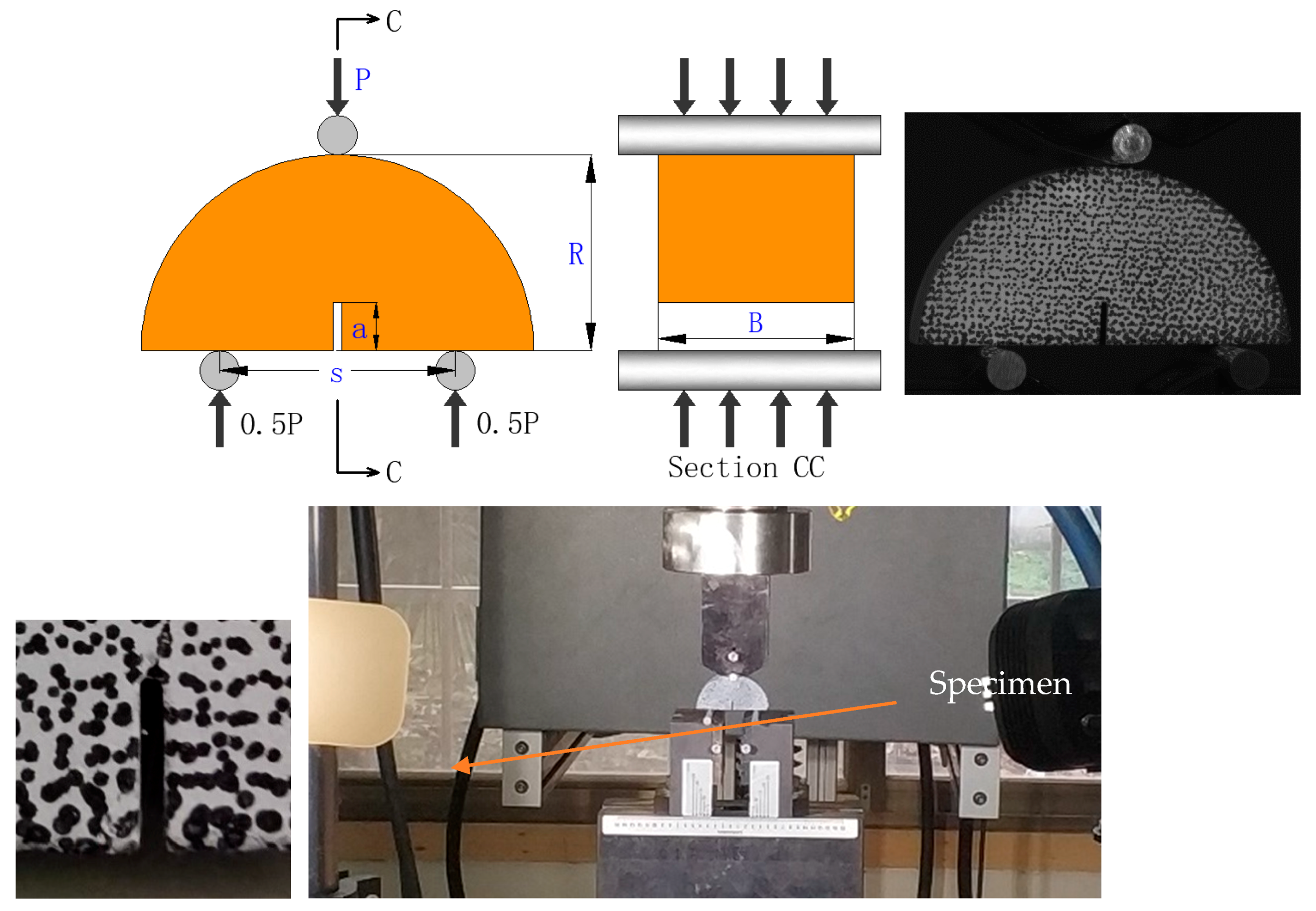
2.1. Specimen and Test Method

The granite material is obtained from Changtai County, Fujian Province, China. The mechanical properties of the granite are shown in

Table 1. Mechanical properties of the granite.

Young’s Modulus	Density	Poisson’s Ratio	P-Wave Velocity	Indirect Tensile Strength	Uniaxial Compressive Strength
40.71 GPa	2790.3 kg/m3	0.23	5345.36 m/s	12.5 MPa	183.3 MPa

.

The loading diagram of SCB granite specimen is shown in Figure 1. A 5 mm long notch is machined at the bottom of the specimen with a cutting machine and the radius of notch tip is 0.5 mm. The corresponding geometric parameters of specimen are listed in

Table 2. Geometrical sizes of granite specimens.

Specimen No.	Radius/mm	Thickness B/mm	Notch Length a/mm	s/mm	${\mathit{Y}}^{\prime } \left(\mathrm{SIF}\right)$
SCB-1	23.37	25.28	5.85	30	3.501
SCB-2	23.56	25.24	5.93	30	3.457
SCB-3	23.64	24.94	6.11	30	3.449

. Test is carried out on MTS Landmark electro-hydraulic servo control material testing machine at Central South University. Load velocity is 1 mm/min.

In addition, the DIC method is applied to record the fracture process of granite specimens. White paint is sprayed on the surface of specimen, and then black speckle is brushed. Speckle diameter on the specimen surface is 0.33 mm (0.013 inches). Two CMOS cameras (GS3-U3-123S6M-C) are used to capture the failure process of granite specimens. The photography frequency is set to 10 fps and takes a picture every 0.1 s. The speckle displacement change is analyzed by a software (Vic-2D 6.0) to determine the evolution of the strain field of the specimen surface. The two cameras are arranged on the left and right sides, and the photos taken by the camera may make it feel that the loading pin is not in the notch line. It can be seen from the last figure in Figure 1 that the loading pin is in notch line.

The calculation formula and processing of test data are based on the suggested method by ISRM. Fracture toughness K_IC of SCB specimen is calculated by Equation (1) [11]:

$${\mathrm{K}}_{\mathrm{IC}}=Y^{\prime }\frac{P_{\max }\sqrt{\pi a}}{2RB},$$

(1)

where

$$Y^{\prime }=-1.297+9.516\frac{s}{2R}-(0.47+16.457\frac{s}{2\mathrm{R}})\frac{a}{R}+(1.071+34.401\frac{s}{2R})\frac{a^2}{R^2}$$

(2)

$P_{\max }$ is the peak load of specimen failure; and $Y^{\prime }$ is dimensionless stress intensity factor.

2.2. Experimental Results

Table 3. The results of Mode I fracture toughness of the granite by the three-point bend test.

Specimen No.	Peak Displacement/mm	Peak Load/KN	KIC/$\mathrm{MPa}\cdot {\mathrm{m}}^{1/2}$	Average of KIC
SCB-1	0.096	4.05	1.627	1.603
SCB-2	0.108	4.00	1.586
SCB-3	0.117	3.94	1.597

lists test results of three SCB specimens, where the peak displacement is displacement corresponding to peak load. The fracture toughness is 1.627, 1.586, and 1.597 $\mathrm{MPa}\cdot {\mathrm{m}}^{1/2}$, respectively, indicating that fracture toughness of the granite is relatively homogeneous. It provides a basis for subsequent numerical simulation.

Figure 2 shows the load–displacement curve of three specimens. The load–displacement curve of three specimens are slightly different due to the difference in geometrical dimensions, but their general shape and variation trend are same. It can be seen that the slope of curve is small during initial loading, and increases significantly with the increase of displacement (after about 0.03 mm). When reaching the peak load point, specimens suddenly fail and load capacity suddenly drops to zero. It is difficult to get a post-peak curve of specimens due to the sudden failure of granite, which is supplemented in the next numerical results.

The post processing of the DIC procedure is as follows: firstly, a study area is selected on the surface of specimen; then, the region is divided into several subsets, and the initial displacements of these subsets are calculated; the corresponding subset is searched based on assumption, and the displacement is calculated; finally, the deformation field of specimen is obtained by processing. The calculation configurations of VIC-2D 6.0 software in DIC post-processing are as follows [32]: subset: 15, step: 4, subset weights: Gaussian weights, error estimation: about 26 $\mathsf{\mu }\mathsf{\epsilon }$, correlation criterion: normalized squared differences.

Figure 3 shows the maximum principal strain evolution process of specimen SCB-1 during the test. It can be seen from Figure 3b,c that the tensile strain zone first occurs at the tip of the notch (indicated by red in the figure), and then tensile strain zone develops rapidly upward, resulting in instantaneous failure of the specimen. When strain reaches about 0.5% (0.005), this area can be regarded as damaged, so the blue-enclosed part in Figure 3c can be considered as the fracture process zone. Figure 3d shows the final failure mode of the specimen; therefore, there is no colorbar. Figure 3e,f show the fracture surface of the specimen.

Due to the rapid failure process of specimen, the static CMOS camera captures a few pictures (10 fps) during the crack propagation process of specimens. The failure process and crack propagation speed are very difficult to obtain accurately, and stress field of the specimen cannot be obtained by the present experiment. Therefore, the FDEM numerical simulation is used in this study to reveal more details during the failure process. The FDEM numerical method has been well applied in rock mechanics. Mahabadi et al. [19] used a coupled finite-discrete element method to simulate behavior of Brazilian disk specimens under dynamic loading. Li et al. [33] studied mechanical properties and the failure process of marble rings under static and dynamic loads by finite-discrete element. The FDEM numerical method can well simulate mechanical properties and the failure process of rocks under external load.

3. Numerical Simulation

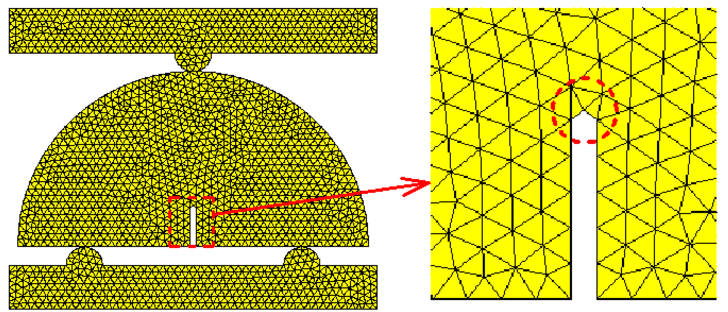
3.1. Numerical Model and Results

The FDEM numerical modeling is performed by software ELFEN. The modeling geometric size is set according to specimen SCB-1 as shown in Figure 4. The radius, thickness, and notch length are 23.37 mm, 25.28 mm, and 5.85 mm, respectively. The model is subdivided into triangular meshes with a side length of 1 mm, and the end of prefabricated notch is sharpened. The international society of rock mechanics and rock engineering recommends that the specimen diameter be more than 10 times the material particle size [11]. The specimen diameter in the numerical model is about 50 mm, larger than 10 times of the mesh size (10 mm), which basically meets the requirements. In addition, the influence of the mesh size on the loading curves is discussed in Appendix A.

The material parameters in model are the same as the granite’s. The material properties and discrete contact parameters are listed in

Table 4. Material properties adopted in the numerical model.

Name	Granite	Loading Platen
Mechanical parameters
Young’s modulus (E, GPa)	40.71	211.00
Poisson’s ratio (μ)	0.23	0.29
Shear modulus (G, Gpa)	16.48	---
Density (ρ,Ns2/mm4)	2.79 × 109	7.84 × 109
Friction angle ($\phi$)	34°
Cohesion (c, MPa)	50
Tensile strength (σt, MPa)	12.5	---
Fracture energy (Gf, N/mm)	0.08	---
Normal penalty (Pn, N/mm2)	8142	211,000
Tangential penalty(Pt, N/mm2)	814	21,100
Discrete contact parameters
Friction of newly generated cracks (γ)	0.65	---
Mesh element size (mm)	1	1
Smallest element size (mm)	0.5	0.5
Contact type	Node-Edge	Node-Edge

. The Mohr–Coulomb criterion with tension cut-off is used to judge the material’s damage as shown in Figure 5, which can judge both tensile and shear fracture of rock. The fracture energy of hard and brittle materials is usually between 0.01 and 0.3 N/mm [19]. Based on previous research, 0.08 N/mm is suitable to describe the hard and brittle granite in this work.

Displacement control is applied on top loading platen. Constant velocity is 0.3 mm/s and strain rate is about 0.012 s⁻¹. Bottom platen is a fixed in the model. Upper platen is a non-fixed with an applied constant velocity.

Figure 6 shows a load–displacement curve of specimens in laboratory and numerical models. The two curves agree well with each other. It indicates that the numerical model can simulate the mechanical properties of granite specimens quite well. Therefore, the numerical simulation is reliable, and it can provide us with more details about the mechanical behavior of specimens.

The simulation is performed quasi-static. The crack is produced when the tensile stress exceeds the tensile strength, and the strain energy reaches the energy required for failure. The length of crack propagation is equal to the strain energy released of the notch divided by the failure energy per unit area of the material. As shown in Figure 7, initial crack is generated from the tip of notch of the specimen, and then grows zigzag toward the top. Eventually, the specimen split into two halves along the middle. Numerical simulation results reproduce failure process of the SCB specimen.

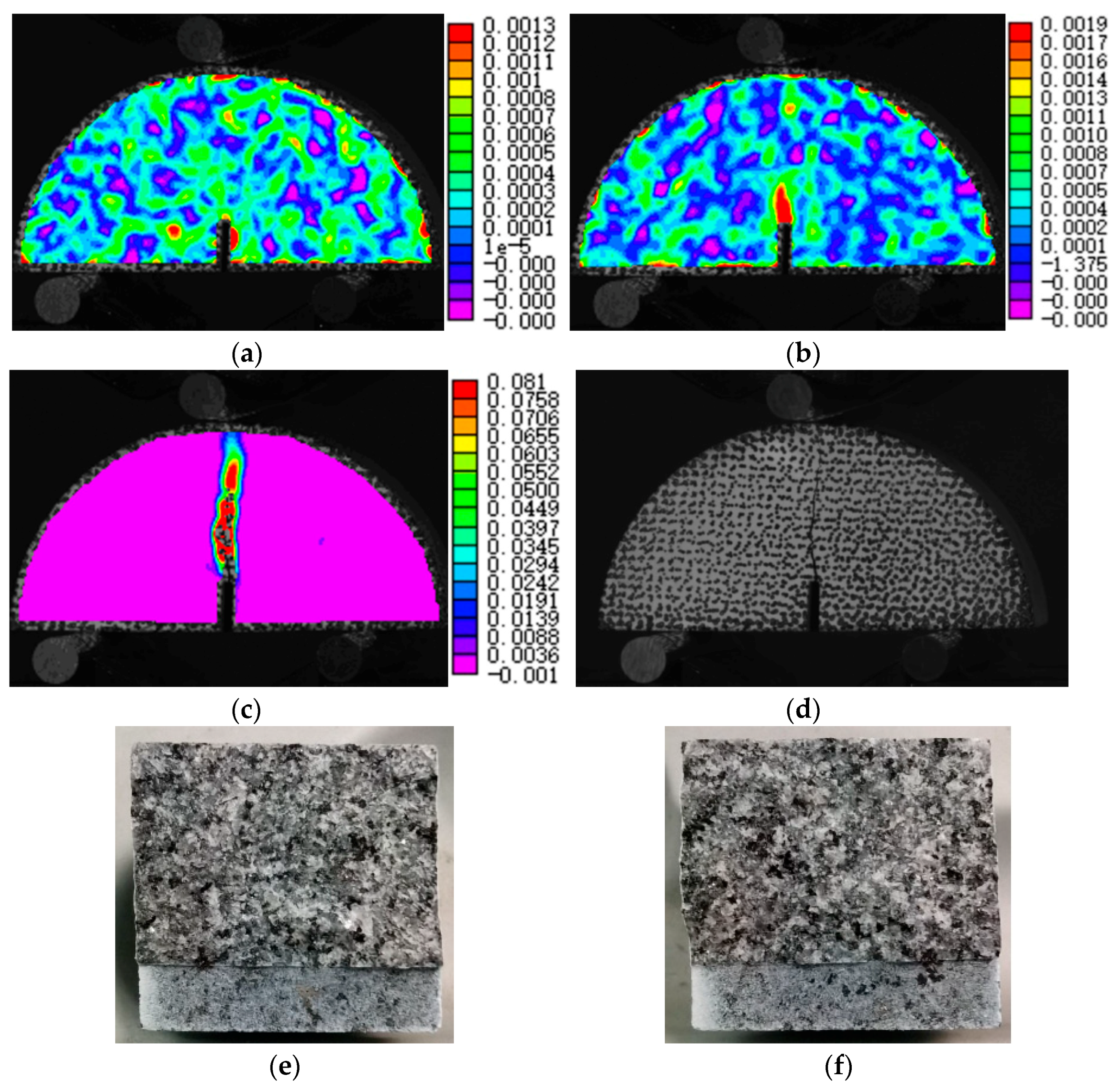
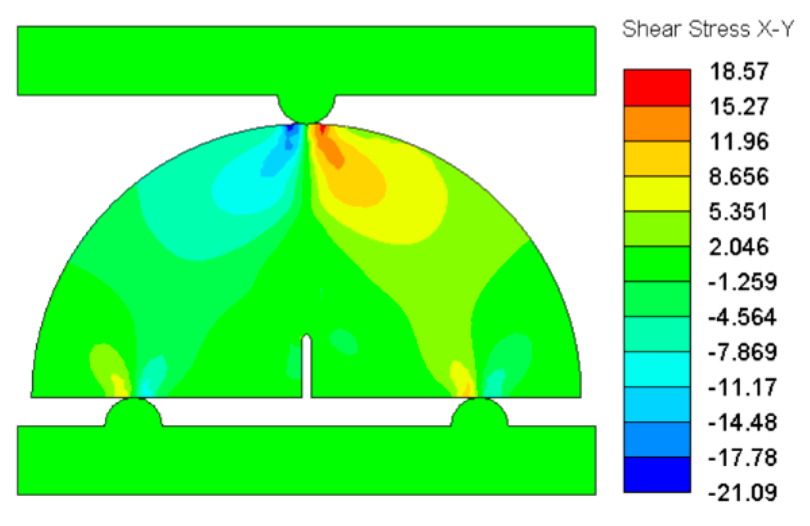
3.2. Stress Field Evolution

During loading process, the stress field on specimen surface can be used to judge the local stress concentration and the overall stress distribution, which is an important information to judge whether the specimen is damaged or not. It is difficult to get the stress field on the surface of specimens in laboratory tests, but the information of the stress field on the surface of specimens can be well obtained in the numerical calculation software.

As shown in Figure 6 and Figure 8, the peak load is 4357 N with the maximum vertical displacement of 0.097 mm under numerical simulation. The specimen is in the tensile state, except the part in contact with platen. The tensile stress concentration is initially created at the tip of pre-notch as shown in Figure 8a. The tensile stress concentration zone of the specimen presents a heart shape at the peak stress point as shown in Figure 8c. After the crack is generated (shown in Figure 8d–f), the maximum tensile stress concentration zone moves up with the crack and expands upward until the crack penetrates the specimen.

For Mode I dominated problems, the failure of rock is dominated by the formation of tensile cracks (Mode I) when the tensile stress exceeds the tensile strength of the material. It can be seen from Figure 9 that the shear stress is concentrated on the top of the specimen and does not cause cracking. The cracks and branches are caused by tensile stress; they are all Mode I crack.

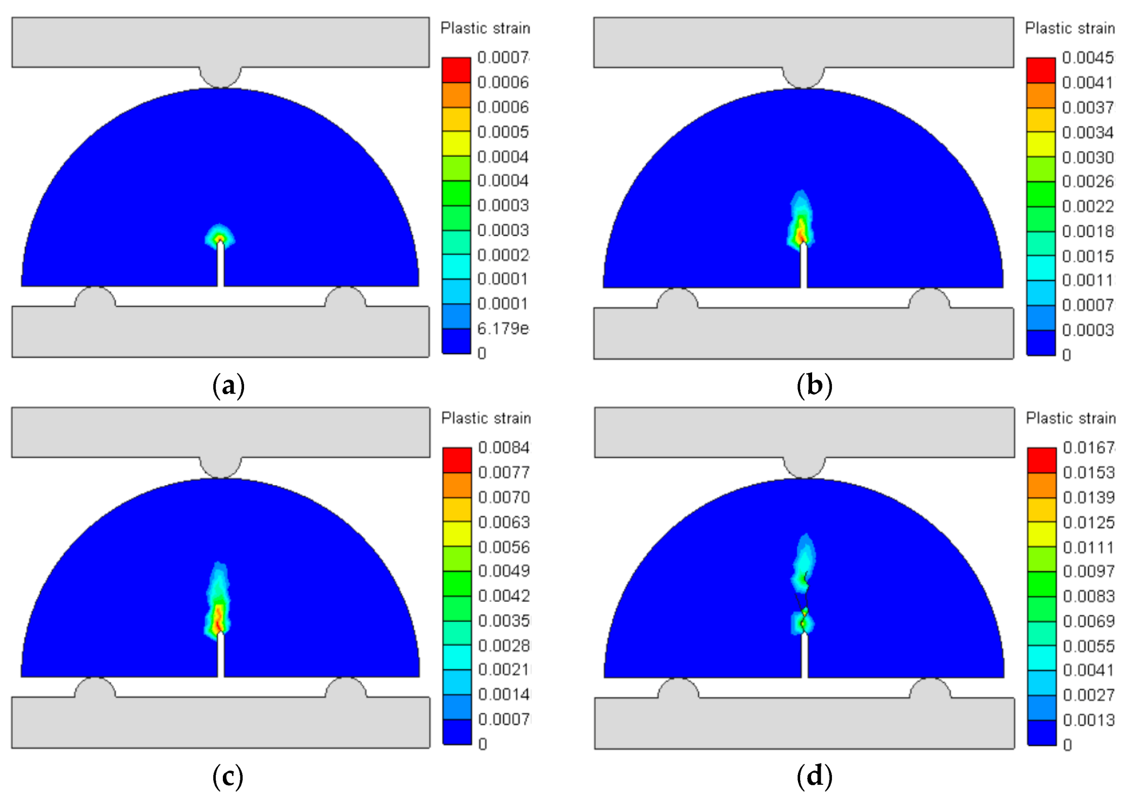
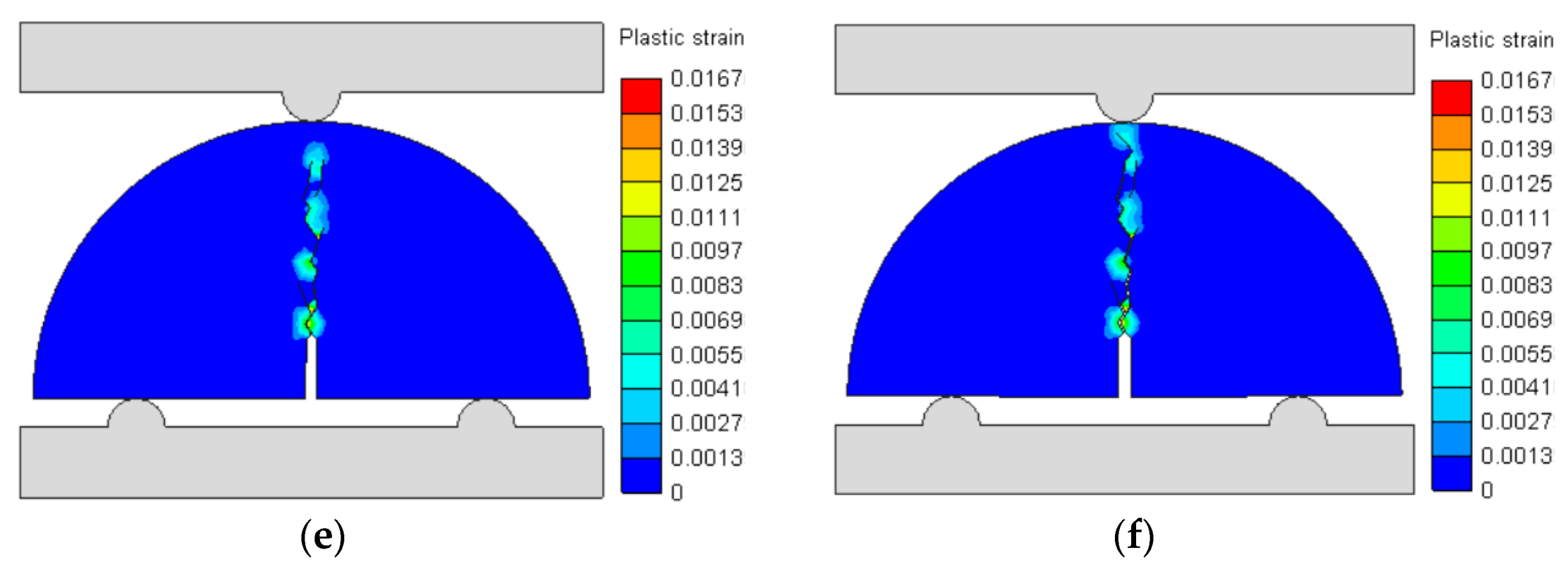
3.3. Evolution of the Fracture Process Zone

The result difference in rock fracture toughness test obtained by different specimen types has attracted the attention of many scholars. Most scholars believe that the fracture process zone (FPZ) near the crack tip is responsible for variation of fracture toughness [35,36,37,38,39]. Therefore, it is necessary to analyze distribution and evolution of the specimen’s FPZ during the loading process, in order to provide more understanding of rock fractures.

The damaging behavior and plastic strain law in the numerical model are shown in Figure 10. During the loading process, the increase of stress causes the elastic strain ${\epsilon }_e$ of material. When the stress of a point reaches the tensile strength ${\sigma }_t$, the elastic strain ${\epsilon }_e$ reaches the maximum ${\epsilon }_e^{peak}$. The strain after the peak elastic strain ${\epsilon }_e^{peak}$ is plastic strain ${\epsilon }_p$. The plastic strain will continue to increase when the energy stored is not enough to produce cracks. The ${\epsilon }_f$ is the strain when the material is fractured. The area $G_f$ under the curve is the energy required for material fracture. When the energy stored is enough to destroy the mesh, the crack will appear in the plastic strain zone.

The plastic strain in the numerical model is shown in Figure 11. The area where the strain reaches about 0.5% (0.005) is considered damaged and can be defined as FPZ. The FPZ is first produced around the tip of the notch and then develops vertically upwards. When the specimen is subjected to a load of 4357 N (peak load), FPZ is obvious (red part as shown in Figure 11b). The plastic strain is about 5 mm, and no macroscopic fractures can be observed at this time. When FPZ (light blue part) grows to about 12 mm as shown in Figure 11d, the tip of the notch began to produce macro fractures inside FPZ. Then, the FPZ continues to develop with loading, and the macro fracture continues to occur inside FPZ. When FPZ penetrates the specimen, the bearing capacity of specimen has been reduced to zero.

From the above analysis, it can be known that FPZ is ahead of macro fractures, and macro fractures are generated after peak load. When FPZ penetrates the specimen, the bearing capacity of specimen has been reduced to 0, and the macro fracture has not completely penetrated the specimen at this time. This indicates FPZ control fracture behavior of the specimen.

3.4. The Crack Propagation Velocity

The crack propagation velocity is an important piece of information in specimen failure. In order to obtain the crack propagation velocity, the crack length was measured every 30 microseconds. Figure 12 shows a relationship between the crack length and the time increment. It can be calculated that the average crack propagation velocity is about 111 m/s. The crack propagation process includes two stages according to crack propagation velocity, namely the rapid crack initiation development stage (A to B) and the final crack splitting stage (B to C). The crack propagates rapidly at the crack initiation development stage and velocity is about 267 m/s, which is also the main stage of the crack formation. The crack propagation velocity is slowed down at the final splitting stage. The crack propagation experienced fast and slow stages in the whole process.

4. Conclusions

The mode I fracture process of the semi-circular bend (SCB) rock specimen is analyzed by experimental and numerical methods in this work. The main conclusions were obtained as follows:

(1)

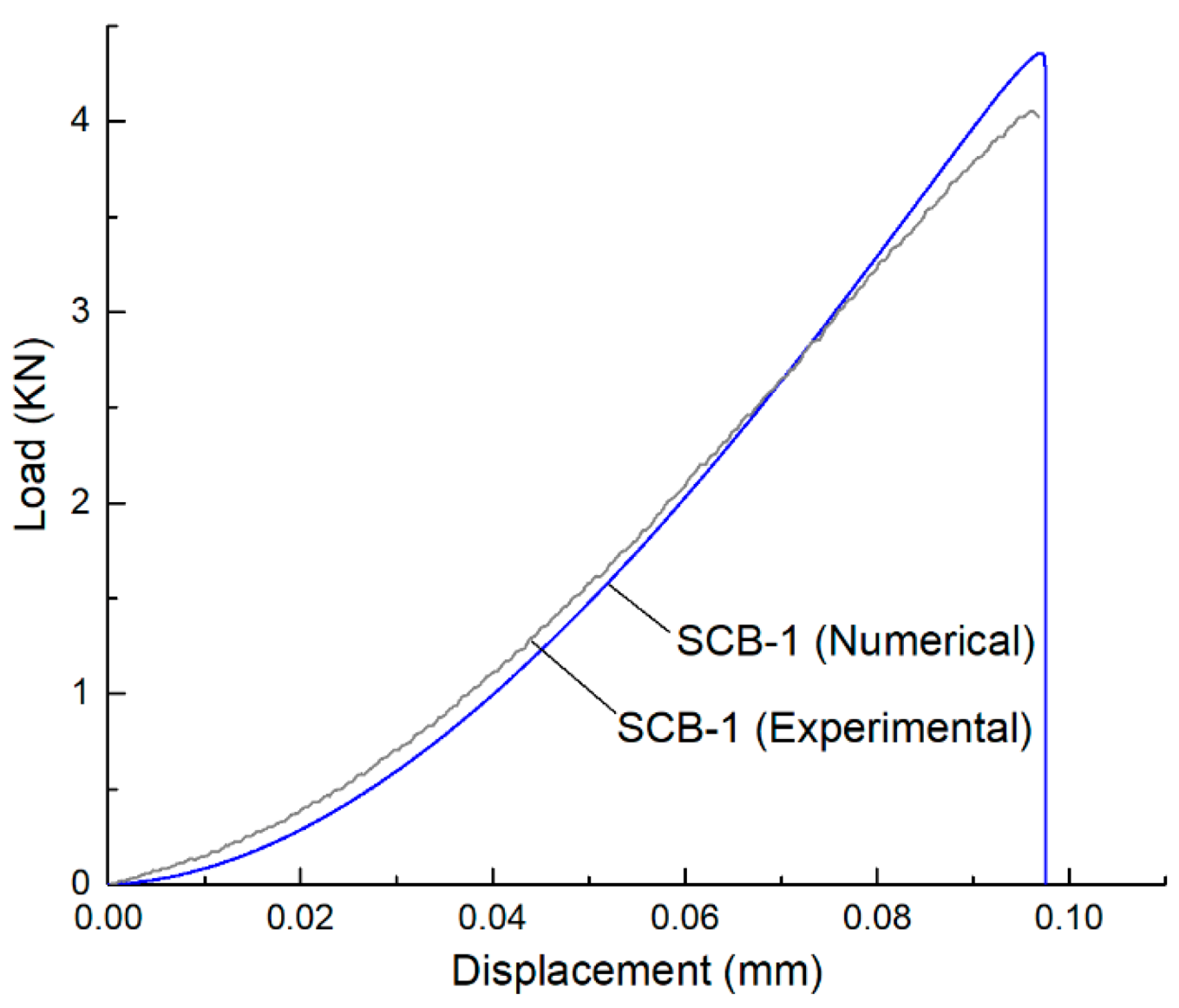
The notch tip of is a SCB specimen, often an arc, which may lead to the change of the crack initiation position. In the numerical model, there is an angle at the notch tip to ensure that the crack initiation position is in the center of tip. The FDEM numerical calculation method can well simulate the mode I failure mode and the stress–strain curve of the SCB specimen. It can provide important information of the mode I failure process, such as the stress field and strain field, which is difficult to obtain in the laboratory test, and provides powerful help for the study of mode I fracture.

(2)

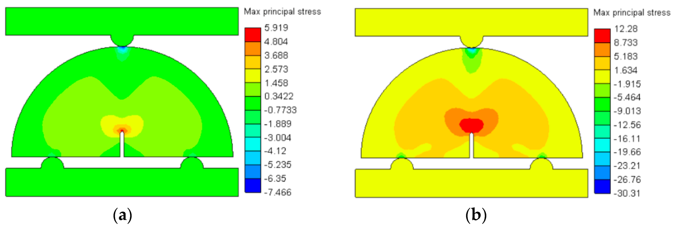
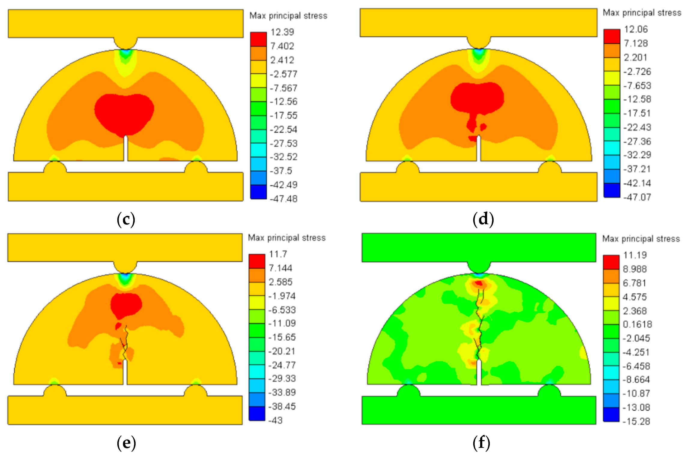
During the loading process, the tensile stress concentration zone of the SCB specimen generates and grows at the notch tip of the specimen. The tensile stress concentration zone of specimens presents a heart shape at peak load. After macro cracks were generated, the maximum tensile stress concentration zone moves upward with crack propagation.

(3)

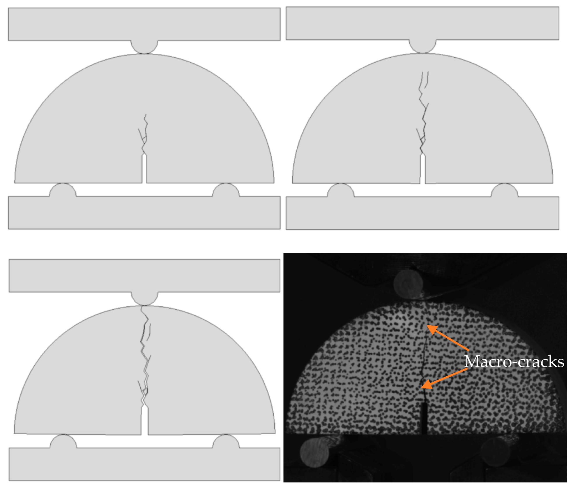
The fracture process zone (FPZ) of the specimen forms before macro fractures under both experimental tests and numerical simulation. The macroscopic fracture forms inside FPZ in the post-peak region of a load–displacement curve. The macroscopic fracture’s length is behind FPZ’s. The FPZ controls fracture behavior of the specimen.

(4)

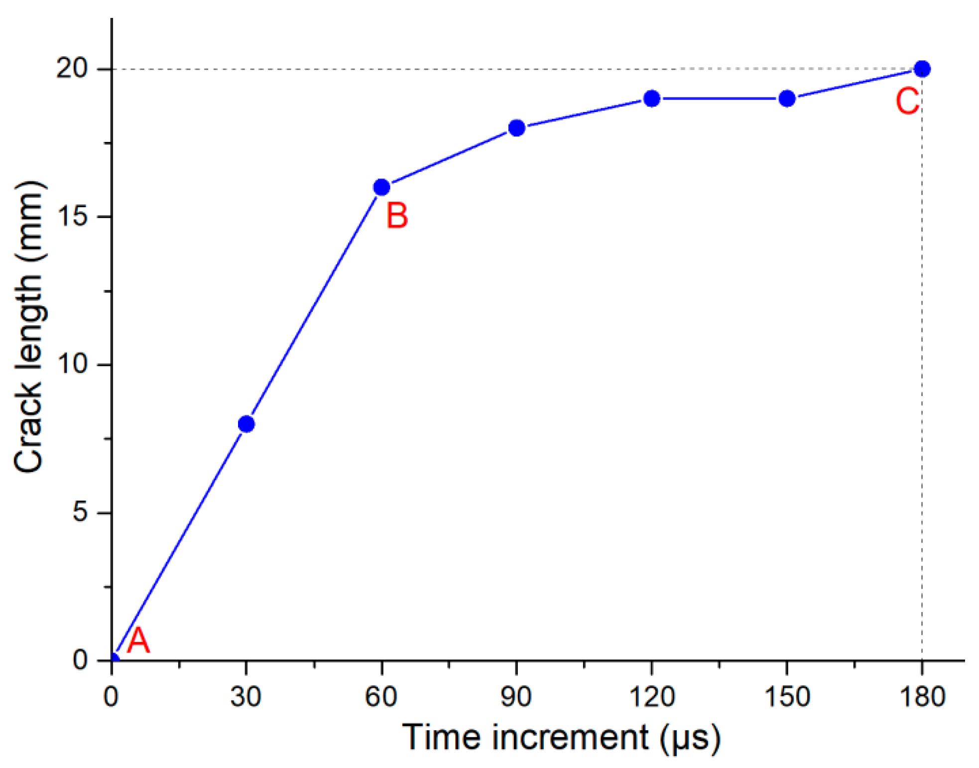
The crack propagation process of the specimen includes two stages according to crack propagation velocity, namely the rapid crack initiation development stage and the final crack splitting stage. The maximum crack propagation velocity is about 267 m/s and the average crack propagation velocity is about 111 m/s.

References

1. Wei, M.; Dai, F.; Xu, N.; Zhao, T. Experimental and numerical investigation of cracked chevron notched Brazilian disc specimen for fracture toughness testing of rock. Fatigue Fract. Eng. Mater. Struct. 2018, 41, 197–211. [Google Scholar] [CrossRef]
2. Zhang, Z. An empirical relation between mode I fracture toughness and the tensile strength of rock. Int. J. Rock Mech. Min. Sci. 2002, 39, 401–406. [Google Scholar] [CrossRef]
3. Zhou, Y.; Xia, K.; Li, X.; Li, H.; Ma, G.; Zhao, J.; Zhou, Z.; Dai, F. Suggested Methods for Determining the Dynamic Strength Parameters and Mode-I Fracture Toughness of Rock Materials. Int. J. Rock Mech. Min. Sci. 2012, 49, 105–112. [Google Scholar] [CrossRef]
4. Yin, T.; Bai, L.; Li, X.; Li, X.; Zhang, S. Effect of thermal treatment on the mode I fracture toughness of granite under dynamic and static coupling load. Eng. Fract. Mech. 2018, 199, 143–158. [Google Scholar] [CrossRef]
5. Zhou, L.; Zhu, Z.; Dong, Y.; Ying, P.; Wang, M. Study of the fracture behavior of mode I and mixed mode I/II cracks in tunnel under impact loads. Tunn. Undergr. Space Technol. 2019, 84, 11–21. [Google Scholar] [CrossRef]
6. Wang, M.; Wang, F.; Zhu, Z.; Dong, Y.; Nezhad, M.M.; Zhou, L. Modelling of crack propagation in rocks under SHPB impacts using a damage method. Fatigue Fract. Eng. Mater. Struct. 2019, 42, 1699–1710. [Google Scholar] [CrossRef]
7. Aliha, M.R.M.; Mahdavi, E.; Ayatollahi, M.R. The Influence of Specimen Type on Tensile Fracture Toughness of Rock Materials. Pure Appl. Geophys. 2017, 174, 1237–1253. [Google Scholar] [CrossRef]
8. Chandler, M.R.; Meredith, P.G.; Brantut, N.; Crawford, B.R. Fracture toughness anisotropy in shale. J. Geophys. Res. Solid Earth 2016, 121, 1706–1729. [Google Scholar] [CrossRef] [Green Version]
9. Needleman, A. Dynamic mode II crack growth along an interface between an elastic solid and a plastic solid. J. Mech. Phys. Solids 2018, 120, 22–35. [Google Scholar] [CrossRef]
10. Gao, G.; Yao, W.; Xia, K.; Li, Z. Investigation of the rate dependence of fracture propagation in rocks using digital image correlation (DIC) method. Eng. Fract. Mech. 2015, 138, 146–155. [Google Scholar] [CrossRef] [Green Version]
11. Kuruppu, M.; Obara, Y.; Ayatollahi, M.R.; Chong, K.P.; Funatsu, T. ISRM-Suggested Method for Determining the Mode I Static Fracture Toughness Using Semi-Circular Bend Specimen. Rock Mech. Rock Eng. 2014, 47, 267–274. [Google Scholar] [CrossRef] [Green Version]
12. Kuruppu, M.; Chong, K. Fracture toughness testing of brittle materials using semi-circular bend (SCB) specimen. Eng. Fract. Mech. 2012, 91, 133–150. [Google Scholar] [CrossRef]
13. Funatsu, T.; Kuruppu, M.; Matsui, K. Effects of temperature and confining pressure on mixed-mode (I–II) and mode II fracture toughness of Kimachi sandstone. Int. J. Rock Mech. Min. Sci. 2014, 67, 1–8. [Google Scholar] [CrossRef]
14. Gao, G.; Huang, S.; Xia, K.; Li, Z. Application of Digital Image Correlation (DIC) in Dynamic Notched Semi-Circular Bend (NSCB) Tests. Exp. Mech. 2015, 55, 95–104. [Google Scholar] [CrossRef]
15. Wei, M.; Dai, F.; Xu, N.-W.; Liu, Y.; Zhao, T. Fracture prediction of rocks under mode I and mode II loading using the generalized maximum tangential strain criterion. Eng. Fract. Mech. 2017, 186, 21–38. [Google Scholar] [CrossRef]
16. Xu, Y.; Dai, F.; Xu, N.W.; Zhao, T. Numerical Investigation of Dynamic Rock Fracture Toughness Determination Using a Semi-Circular Bend Specimen in Split Hopkinson Pressure Bar Testing. Rock Mech. Rock Eng. 2016, 49, 731–745. [Google Scholar] [CrossRef]
17. Dai, F.; Wei, M.; Xu, N.; Zhao, T.; Xu, Y. Numerical investigation of the progressive fracture mechanisms of four ISRM-suggested specimens for determining the mode I fracture toughness of rocks. Comput. Geotech. 2015, 69, 424–441. [Google Scholar] [CrossRef]
18. Wei, M.; Dai, F.; Xu, N.; Zhao, T.; Xia, K. Experimental and numerical study on the fracture process zone and fracture toughness determination for ISRM-suggested semi-circular bend rock specimen. Eng. Fract. Mech. 2016, 154, 43–56. [Google Scholar] [CrossRef]
19. Mahabadi, O.; Cottrell, B.; Grasselli, G. An example of realistic modelling of rock dynamics problems: FEM/DEM simulation of dynamic Brazilian test on Barre granite. Rock Mech. Rock Eng. 2010, 43, 707–716. [Google Scholar] [CrossRef]
20. Rougier, E.; Knight, E.E.; Sussman, A.J.; Swift, R.P.; Bradley, C.R.; Munjiza, A.; Broome, S.T. The combined finite-discrete element method applied to the study of rock fracturing behavior in 3D. In Proceedings of the 45th US Rock Mechanics/Geomechanics Symposium, San Francisco, CA, USA, 26–29 June 2011. [Google Scholar]
21. Cai, M. Fracture initiation and propagation in a Brazilian disc with a plane interface: A numerical study. Rock Mech. Rock Eng. 2013, 46, 289–302. [Google Scholar] [CrossRef]
22. Feng, F.; Li, X.; Li, D. Modeling of failure characteristics of rectangular hard rock influenced by sample height-to-width ratios: A finite/discrete element approach. Comptes Rendus Mécanique 2017, 345, 317–328. [Google Scholar] [CrossRef]
23. Okubo, K.; Bhat, H.S.; Rougier, E.; Marty, S.; Schubnel, A.; Lei, Z.; Knight, E.E.; Klinger, Y. Dynamics, Radiation, and Overall Energy Budget of Earthquake Rupture with Coseismic Off-Fault Damage. J. Geophys. Res. Solid Earth 2019, 124, 11771–11801. [Google Scholar] [CrossRef] [Green Version]
24. Kondori, B.; Benzerga, A.A.; Needleman, A. Discrete shear-transformation-zone plasticity modeling of notched bars. J. Mech. Phys. Solids 2018, 111, 18–42. [Google Scholar] [CrossRef]
25. Zhu, Q.; Li, D.; Han, Z.; Li, X.; Zhou, Z. Mechanical properties and fracture evolution of sandstone specimens containing different inclusions under uniaxial compression. Int. J. Rock Mech. Min. Sci. 2019, 115, 33–47. [Google Scholar] [CrossRef]
26. Dong, W.; Wu, Z.; Zhou, X.; Wang, N.; Kastiukas, G. An experimental study on crack propagation at rock-concrete interface using digital image correlation technique. Eng. Fract. Mech. 2017, 171, 50–63. [Google Scholar] [CrossRef]
27. Xiao, P.; Li, D.; Zhao, G.; Zhu, Q.; Liu, H.; Zhang, C. Mechanical properties and failure behavior of rock with different flaw inclinations under coupled static and dynamic loads. J. Cent. South Univ. 2020, 27, 2945–2958. [Google Scholar] [CrossRef]
28. Rethore, J.; Estevez, R. Identification of a cohesive zone model from digital images at the micron-scale. J. Mech. Phys. Solids 2013, 61, 1407–1420. [Google Scholar] [CrossRef]
29. Romani, R.; Bornert, M.; Leguillon, D.; Le Roy, R.; Sab, K. Detection of crack onset in double cleavage drilled specimens of plaster under compression by digital image correlation—Theoretical predictions based on a coupled criterion. Eur. J. Mech. A-Solids 2015, 51, 172–182. [Google Scholar] [CrossRef]
30. Roux, S.; Rethore, J.; Hild, F. Digital image correlation and fracture: An advanced technique for estimating stress intensity factors of 2D and 3D cracks. J. Phys. D-Appl. Phys. 2009, 42. [Google Scholar] [CrossRef] [Green Version]
31. Dautriat, J.; Bornert, M.; Gland, N.; Dimanov, A.; Raphanel, J. Localized deformation induced by heterogeneities in porous carbonate analysed by multi-scale digital image correlation. Tectonophysics 2011, 503, 100–116. [Google Scholar] [CrossRef]
32. Xing, H.Z.; Zhang, Q.B.; Ruan, D.; Dehkhoda, S.; Lu, G.X.; Zhao, J. Full-field measurement and fracture characterisations of rocks under dynamic loads using high-speed three-dimensional digital image correlation. Int. J. Impact Eng. 2018, 113, 61–72. [Google Scholar] [CrossRef]
33. Li, X.; Feng, F.; Li, D. Numerical simulation of rock failure under static and dynamic loading by splitting test of circular ring. Eng. Fract. Mech. 2018, 188, 184–201. [Google Scholar] [CrossRef]
34. Labuz, J.; Zang, A. Mohr-Coulomb failure criterion. Rock Mech. Rock Eng. 2012, 45, 227–231. [Google Scholar] [CrossRef] [Green Version]
35. Wei, M.; Dai, F.; Xu, N.-W.; Zhao, T. Stress intensity factors and fracture process zones of ISRM-suggested chevron notched specimens for mode I fracture toughness testing of rocks. Eng. Fract. Mech. 2016, 168, 174–189. [Google Scholar] [CrossRef]
36. Xu, S.; Malik, M.A.; Li, Q.; Wu, Y. Determination of double-K fracture parameters using semi-circular bend test specimens. Eng. Fract. Mech. 2016, 152, 58–71. [Google Scholar] [CrossRef]
37. Nallathambi, P.; Karihaloo, B. Determination of the specimen size independent fracture toughness of plain concrete. Mag. Concr. Res. 1986, 38, 67–76. [Google Scholar] [CrossRef]
38. Jenq, Y.; Shah, S. Two-parameter fracture model for concrete. ASCE J. Eng. Mech. 1985, 111, 1227–1241. [Google Scholar] [CrossRef]
39. Xu, S.; Reinhardt, H. Determination of double-K criterion for crack propagation in quasi-brittle materials, Part I: Experimental investigation of crack propagation. Int. J. Fract. 1999, 98, 111–149. [Google Scholar] [CrossRef]
Figure 1. Loading diagram of the SCB specimen (Note: R is radius of specimen; B is thickness; a is notch length; s is distance between two supporting rollers; P is applied load).
Mathematics 09 01769 g001
Figure 2. Load–displacement curve of the laboratory test.
Mathematics 09 01769 g002
Figure 3. The maximum principal strain evolution process and failure mode of specimen SCB-1. (a) 5.6 s; (b) 5.7 s; (c) 5.8 s; (d) failure mode; (e,f) fracture surface.
Mathematics 09 01769 g003
Figure 4. Model geometry and meshes of the SCB-3 specimen test.
Mathematics 09 01769 g004
Figure 5. Mohr–Coulomb criterion with tension cut-off [34].
Mathematics 09 01769 g005
Figure 6. Load–displacement curve.
Mathematics 09 01769 g006
Figure 7. The crack evolution process of numerical simulation and actual failure mode.
Mathematics 09 01769 g007
Figure 8. The maximum principal stress evolution at different loads: (a) 720 N; (b) 2884 N; (c) 4357 N (100% peak); (d) 4153 N (Post peak); (e) 3537 N (Post peak); (f) 1849 N (Post peak) (Note: positive stress value represents tensile stress, and the unit is MPa).
Mathematics 09 01769 g008aMathematics 09 01769 g008b
Figure 9. The shear stress at the peak load and the unit is MPa.
Mathematics 09 01769 g009
Figure 10. The damaging behavior and plastic strain law in the numerical model.
Mathematics 09 01769 g010
Figure 11. Plastic strain evolution at different loads: (a) 2838 N; (b) 4357 N (peak load); (c) 4152 N (post peak); (d) 3537 N; (e) 1849 N; and (f) 0 N.
Mathematics 09 01769 g011aMathematics 09 01769 g011b
Figure 12. The relationship of crack length and the loading time increment.
Mathematics 09 01769 g012