
Fixed-Time Third-Order Super-Twisting-like Sliding Mode Motion Control for Piezoelectric Nanopositioning Stage


Abstract
:1. Introduction
2. Problem Formulation
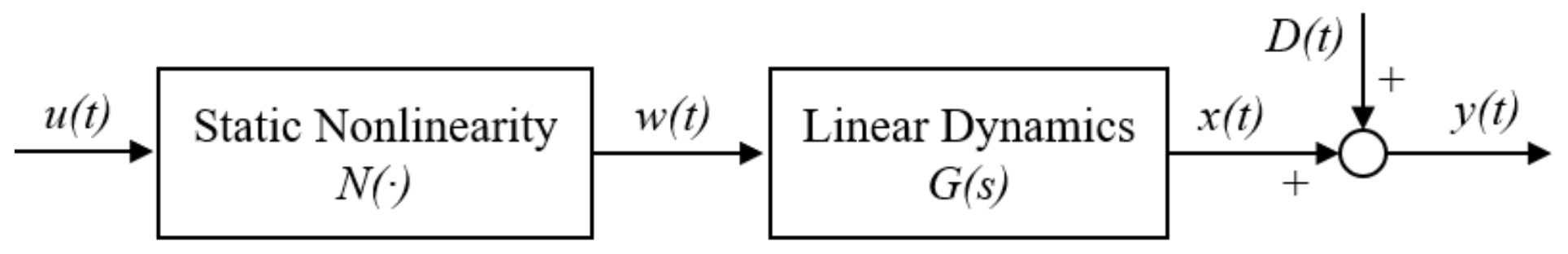
2.1. Dynamical Model
2.2. Disturbance Estimation
3. Design of Controller
4. Simulation Results
5. Conclusions
Author Contributions
Funding
Institutional Review Board Statement
Informed Consent Statement
Conflicts of Interest
References
- Wang, K.; Ruppert, M.G.; Manzie, C.; Nešić, D.; Yong, Y.K. Adaptive scan for atomic force microscopy based on online optimization: Theory and experiment. IEEE Trans. Control Syst. Technol. 2019, 28, 869–883. [Google Scholar] [CrossRef]
- Li, L.; Huang, J.; Aphale, S.S.; Zhu, L. A smoothed raster scanning trajectory based on acceleration-continuous B-spline transition for high-speed Atomic Force Microscopy. IEEE/ASME Trans. Mechatron. 2020, 26, 24–32. [Google Scholar] [CrossRef]
- Wang, G.; Xu, Q. Design and precision position/force control of a piezo-driven microinjection system. IEEE/ASME Trans. Mechatron. 2017, 22, 1744–1754. [Google Scholar] [CrossRef]
- Zhu, Z.; Chen, L.; Huang, P.; Schönemann, L.; Riemer, O.; Yao, J.; To, S.; Zhu, W.L. Design and Control of a Piezoelectrically Actuated Fast Tool Servo for Diamond Turning of Microstructured Surfaces. IEEE Trans. Ind. Electron. 2019, 67, 6688–6697. [Google Scholar] [CrossRef]
- Son, N.N.; Van Kien, C.; Anh, H.P.H. Parameters identification of Bouc–Wen hysteresis model for piezoelectric actuators using hybrid adaptive differential evolution and Jaya algorithm. Eng. Appl. Artif. Intell. 2020, 87, 103317. [Google Scholar] [CrossRef]
- Fan, Y.; Tan, U.X. Design of a Feedforward-Feedback Controller for a Piezoelectric-Driven Mechanism to Achieve High-Frequency Nonperiodic Motion Tracking. IEEE/ASME Trans. Mechatron. 2019, 24, 853–862. [Google Scholar] [CrossRef]
- Gu, G.Y.; Zhu, L.M.; Su, C.Y.; Ding, H.; Fatikow, S. Modeling and control of piezo-actuated nanopositioning stages: A survey. IEEE Trans. Autom. Sci. Eng. 2014, 13, 313–332. [Google Scholar] [CrossRef]
- Wong, P.K.; Xu, Q.; Vong, C.M.; Wong, H.C. Rate-dependent hysteresis modeling and control of a piezostage using online support vector machine and relevance vector machine. IEEE Trans. Ind. Electron. 2011, 59, 1988–2001. [Google Scholar] [CrossRef]
- Meng, D.; Xia, P.; Lang, K.; Smith, E.C.; Rahn, C.D. Neural Network Based Hysteresis Compensation of Piezoelectric Stack Actuator Driven Active Control of Helicopter Vibration. Sens. Actuators A Phys. 2020, 302, 111809. [Google Scholar] [CrossRef]
- Zhang, C.; Dai, M.Z.; Wu, J.; Xiao, B.; Li, B.; Wang, M. Neural-networks and event-based fault-tolerant control for spacecraft attitude stabilization. Aerosp. Sci. Technol. 2021, 114, 106746. [Google Scholar] [CrossRef]
- Ang, W.T.; Khosla, P.K.; Riviere, C.N. Feedforward controller with inverse rate-dependent model for piezoelectric actuators in trajectory-tracking applications. IEEE/ASME Trans. Mechatron. 2007, 12, 134–142. [Google Scholar] [CrossRef] [Green Version]
- Zhu, W.; Rui, X.T. Hysteresis modeling and displacement control of piezoelectric actuators with the frequency-dependent behavior using a generalized Bouc–Wen model. Precis. Eng. 2016, 43, 299–307. [Google Scholar] [CrossRef]
- Zhang, C.; Wang, J.; Zhang, D.; Shao, X. Fault-tolerant adaptive finite-time attitude synchronization and tracking control for multi-spacecraft formation. Aerosp. Sci. Technol. 2018, 73, 197–209. [Google Scholar] [CrossRef]
- Polyakov, A. Nonlinear feedback design for fixed-time stabilization of linear control systems. IEEE Trans. Autom. Control 2011, 57, 2106–2110. [Google Scholar] [CrossRef] [Green Version]
- Sun, R.; Shan, A.; Zhang, C.; Wu, J.; Jia, Q. Quantized fault-tolerant control for attitude stabilization with fixed-time disturbance observer. J. Guid. Control Dyn. 2021, 44, 449–455. [Google Scholar] [CrossRef]
- Zhang, C.; Wu, J.; Sun, R.; Wang, M.; Ran, D. Actuator Model for Spacecraft Attitude Control Simulation. Aircr. Eng. Aerosp. Technol. 2021, 93, 553–557. [Google Scholar] [CrossRef]
- Kamal, S.; Chalanga, A.; Moreno, J.A.; Fridman, L.; Bandyopadhyay, B. Higher order super-twisting algorithm. In Proceedings of the 2014 13th International Workshop on Variable Structure Systems (VSS), Nantes, France, 29 June–2 July 2014; pp. 1–5. [Google Scholar]
- Lu, B.; Fang, Y.; Sun, N. Continuous sliding mode control strategy for a class of nonlinear underactuated systems. IEEE Trans. Autom. Control 2018, 63, 3471–3478. [Google Scholar] [CrossRef]
- Xu, Q. Adaptive Integral Terminal Third-Order Finite-Time Sliding-Mode Strategy for Robust Nanopositioning Control. IEEE Trans. Ind. Electron. 2020, 68, 6161–6170. [Google Scholar] [CrossRef]
- Yang, J.; Li, S.; Yu, X. Sliding-mode control for systems with mismatched uncertainties via a disturbance observer. IEEE Trans. Ind. Electron. 2012, 60, 160–169. [Google Scholar] [CrossRef]
- Xu, Q. Continuous integral terminal third-order sliding mode motion control for piezoelectric nanopositioning system. IEEE/ASME Trans. Mechatron. 2017, 22, 1828–1838. [Google Scholar] [CrossRef]
- Basin, M.; Panathula, C.B.; Shtessel, Y. Multivariable continuous fixed-time second-order sliding mode control: Design and convergence time estimation. IET Control Theory Appl. 2016, 11, 1104–1111. [Google Scholar] [CrossRef]
- Elmali, H.; Olgac, N. Implementation of sliding mode control with perturbation estimation (SMCPE). IEEE Trans. Control Syst. Technol. 1996, 4, 79–85. [Google Scholar] [CrossRef]
- Bhat, S.P.; Bernstein, D.S. Finite-time stability of continuous autonomous systems. SIAM J. Control Optim. 2000, 38, 751–766. [Google Scholar] [CrossRef]
- Zuo, Z.; Han, Q.L.; Ning, B. Fixed-Time Cooperative Control of Multi-Agent Systems; Springer: Berlin/Heidelberg, Germany, 2019. [Google Scholar]


| Parameter | ||||||||
|---|---|---|---|---|---|---|---|---|
| Value | 2 | 0.6 | 3 | 10 | 8 | 340 |
| Controller Type | 5 Hz Sinewave | 10 Hz Sinewave | 20 Hz Sinewave | 50 Hz Sinewave |
|---|---|---|---|---|
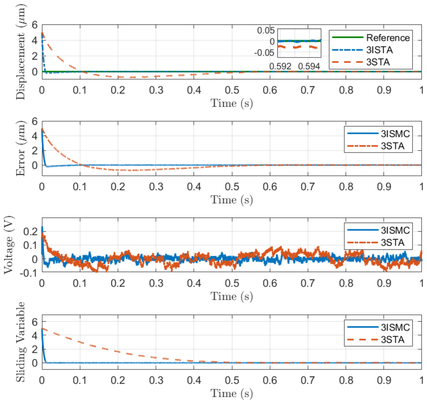
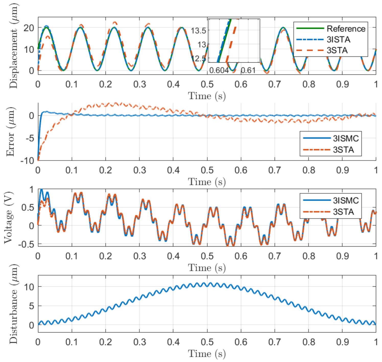
| 3-STA (μm) | 1.7782 | 1.7780 | 1.7778 | 4.3219 |
| 3-ISMC (μm) | 0.5914 | 0.5188 | 0.9703 | 0.7348 |
Publisher’s Note: MDPI stays neutral with regard to jurisdictional claims in published maps and institutional affiliations. |
© 2021 by the authors. Licensee MDPI, Basel, Switzerland. This article is an open access article distributed under the terms and conditions of the Creative Commons Attribution (CC BY) license (https://creativecommons.org/licenses/by/4.0/).
Share and Cite
Wang, G.; Wang, B.; Zhang, C. Fixed-Time Third-Order Super-Twisting-like Sliding Mode Motion Control for Piezoelectric Nanopositioning Stage. Mathematics 2021, 9, 1770. https://doi.org/10.3390/math9151770
Wang G, Wang B, Zhang C. Fixed-Time Third-Order Super-Twisting-like Sliding Mode Motion Control for Piezoelectric Nanopositioning Stage. Mathematics. 2021; 9(15):1770. https://doi.org/10.3390/math9151770
Chicago/Turabian StyleWang, Guangwei, Bo Wang, and Chengxi Zhang. 2021. "Fixed-Time Third-Order Super-Twisting-like Sliding Mode Motion Control for Piezoelectric Nanopositioning Stage" Mathematics 9, no. 15: 1770. https://doi.org/10.3390/math9151770