Particle Filtering: A Priori Estimation of Observational Errors of a State-Space Model with Linear Observation Equation ^†

Abstract

Observational errors of Particle Filtering are studied over the case of a state-space model with a linear observation equation. In this study, the observational errors are estimated prior to the upcoming observations. This action is added to the basic algorithm of the filter as a new step for the acquisition of the state estimations. This intervention is useful in the presence of missing data problems mainly, as well as sample tracking for impoverishment issues. It applies theory of Homogeneous and Non-Homogeneous closed Markov Systems to the study of particle distribution over the state domain and, thus, lays the foundations for the employment of stochastic control against impoverishment. A simulating example is quoted to demonstrate the effectiveness of the proposed method in comparison with existing ones, showing that the proposed method is able to combine satisfactory precision of results with a low computational cost and provide an example to achieve impoverishment prediction and tracking.

1. Introduction

Particle Filter (PF) methodology deals with the estimation of latent variables of stochastic processes taking into consideration noisy observations generated by the latent variables [1]. This technique mainly consists of Monte-Carlo (MC) simulation [2] of the hidden variables and the weight assignment to the realizations of the random trials during simulation, the particles. This procedure is repeated sequentially, at every time step of a stochastic process. The involvement of sequential MC simulation in the method is accompanied by a heavy computational cost. However, the nature of the MC simulation makes the PF estimation methodology suitable for a wide variety of state-space models, including non-linear models with non-Gaussian noise. The weights are defined according to observations, which are received at every time step. The weight assignment step constitutes an evaluation process of the existing particles, which are created at the simulation step.

As weight assignment according to an observation dataset is a substantial part of PF, missing observations hinder the function of the filter. Wang et al. [3] wrote a review concerning PF on target tracking, wherein they mentioned cases of missing data and measurement uncertainties within multi-target tracking, as well as methods that deal with this problem (see, e.g., [4]). Techniques that face the problem of missing data focus mainly on substitution of the missing data. In recent decades, Expectation-Maximization algorithm [5] and Markov-Chain Monte Carlo methods [6] became popular for handling missing data problems. These algorithms have been constructed independently of PF. Gopaluni [7] proposed a combination of Expectation-Maximization algorithm with PF for parameter estimation with missing data. Housfater et al. [8] devised Multiple Imputations Particle Filter (MIPF), wherein missing data are substituted by multiple imputations from a proposal distribution and these imputations are evaluated with an additional weight assignment according to their proposal distribution. Xu et al. [9] involved uncertainty on data availability in the observations with the form of additional random variables in the subject state-space model. All the aforementioned approaches are powerful, although computationally costly.

This paper focuses on state-space models with linear observation equations and provides an estimation of the errors of missing observations (in cases of missing data), aiming at the approximation of weights, under a Missing At Random (MAR) assumption [10]. Linearity in an observation equation permits sequential replacements of missing values with equal quantities of known distributions. Although this method is applicable to a smaller set of models than the former ones, it is much faster as it leads to a single imputation process. A simulating example is provided for the comparison of the suggested method with existing techniques for the advantages of the proposed algorithm to be highlighted. The contribution of the a priori estimation step to the study of impoverishment phenomena is also exhibited through Markov System (MS) framework (see, e.g., [11]). The substitution of future weights renders the estimation of future distribution of particles in the state domain feasible. The significance of this initiative lays on the possible estimation of the sample condition concerning impoverishment, in future steps, based on the suggested theory. Such a practice permits the coordinated application of stochastic control [12] instead of the mostly empirical approaches that been proposed so far [13].

The present article is based on the work of Lykou and Tsaklidis [14]. Further mathematical propositions are formed by the sparse remarks exhibited in [14], and the incorporation procedure of MS-theory in the study of particle distribution is explained in detail. The presentation of the initial results of the simulation example is reformulated for the example to be more easily understandable, as well as a new application of MS-theory for the quantitative prior estimation of the particle distribution one time step forward is added to the initial example. In Section 2, PF algorithm is presented analytically. In Section 3, the new weight estimation step is introduced and its connection with the study of degeneracy and impoverishment is explained. In Section 4, a simulating example is provided, where the results of the current method are compared with those of MIPF and the results of the basic PF algorithm in the case when all data are available. An example for the estimation of the particle distribution one step ahead after the current is also presented in the direction of impoverishment tracking and prediction. In Section 5, the discussion and concluding remarks are quoted.

2. Particle Filter Algorithm

Let ${\left\{x_t\right\}}_{t\in \mathbb{N}}$ be a stochastic process described by m-dimensional latent vectors, $x_t\in {\mathbb{R}}^m$, and ${\left\{y_t\right\}}_{t\in \mathbb{N}}$ be the k-dimensional process of noisy observations, $y_t\in {\mathbb{R}}^k$. The states and observations are inter-related according to the state-space model,

$$\begin{array}{ccc}\hfill x_t& =& f\left(x_{t-1}\right)+v_t\hfill \end{array}$$

(1)

$$\begin{array}{ccc}\hfill y_t& =& c+A{x}_t+u_t\iff y_t-c-A{x}_t=u_t.\hfill \end{array}$$

(2)

In the system of Equations (1) and (2), f is a known deterministic function of $x_t$, $v_t$ stands for the process noise, and $u_t$ symbolizes the observation noise. Each sequence ${\left\{v_t\right\}}_{t\in \mathbb{N}}$ and ${\left\{u_t\right\}}_{t\in \mathbb{N}}$ consists of independent and identically distributed (iid) random vectors, while $c\in {\mathbb{R}}^k$ is a constant vector and $A\in {\mathbb{R}}^{k\times m}$ is a constant matrix.

PF methodology employs Bayesian inference for state estimation. The Bayesian approach aims at the construction of the posterior probability distribution function $p\left(x_t\right|y_{1:t})$, where $y_{1:t}=(y_1,y_2,\dots ,y_t)$, resorting to the recursive equations,

$$\begin{array}{ccc}\hfill p\left(x_t\right|y_{1:t-1})& =& \int p\left(x_t\right|x_{t-1})p\left(x_{t-1}\right|y_{1:t-1})d{x}_{t-1}\left(\mathrm{prediction}\right)\hfill \\ \hfill p\left(x_t\right|y_{1:t})& =& \frac{p\left(y_t\right|x_t)p\left(x_t\right|y_{1:t-1})}{\int p\left(y_t\right|x_t^{\prime })p\left(x_t^{\prime }\right|y_{1:t-1})d{x}_t^{\prime }}\left(\mathrm{update}\right).\hfill \end{array}$$

These equations are analytically solvable in cases of linear state-space models with Gaussian noises. However, for more general models, analytical solutions are usually infeasible. For this reason, PF can be applied by utilizing MC simulation and integration to represent the state posterior probability distribution function, $p\left(x_t\right|y_{1:t})$, with the help of a set of $N\in \mathbb{N}$ particles $x_t^i$, $i=1,2,\dots ,N$, with corresponding weights $w_t^i$, $i=1,2,\dots ,N$. Then, $p\left(x_t\right|y_{1:t})$ can be approximated by the discrete mass probability distribution of the weighted particles ${\left\{x_t^i\right\}}_{i=1}^N$ as

$$\widehat{p}\left(x_t\right|y_{1:t})\approx \sum _{i=1}^N{w}_t^i\delta (x_t-x_t^i),$$

where $\delta$ is the Dirac delta function and weights are normalized, so that ${\sum }_i{w}_k^i=1$. As $p\left(x_t\right|y_{1:t})$ is usually unknown; this MC simulation is based on importance sampling, namely a known probability (importance) density $q\left(x_t\right|y_{1:t})$ is chosen in order for the set of particles to be produced. Then, the state posterior distribution is approximated by

$$\widehat{p}\left(x_t\right|y_{1:t})\approx \sum _{i=1}^N{\tilde{w}}_t^i\delta (x_t-{\tilde{x}}_t^i),$$

with ${\tilde{x}}_t^i\sim q\left(x_t\right|y_{1:t})$, while

$${\tilde{w}}_t^i\propto {\tilde{w}}_{t-1}^i\frac{p\left(y_t\right|{\tilde{x}}_t^i)p\left({\tilde{x}}_t^i\right|{\tilde{x}}_{t-1}^i)}{q\left({\tilde{x}}_t^i\right|{\tilde{x}}_{t-1}^i,y_t)}$$

(3)

are the normalized particle weights for $i=1,2,\dots ,N$.

As PF is applied successively for several time steps, it happens that increasing weights are assigned to the most probable particles, while the weights of the other particles become negligible progressively. Thus, only a very small proportion of particles is finally used for the state estimation. This phenomenon is known as PF degeneracy. In order to face this problem, a resampling with replacement step according to the calculated weights has been incorporated into the initial algorithm, resulting in the Sampling Importance Resampling (SIR) algorithm. Nevertheless, sequential resampling leads the particles to take values from a very small domain and exclude many other less probable values. This problem is called impoverishment. A criterion over the weight variability has been introduced for a decision to be made at every time step, whether existing particles should be resampled or not, to reach the middle ground between degeneracy and impoverishment. In this criterion, the Effective Sample Size measure of degeneracy, defined as

$$N_{eff}\left(t\right)=\frac{N}{1+Va{r}_{p(•|y_{1:t})}\left(w\left(x_t\right)\right)},$$

is involved (see, e.g., [15], pp. 35–36). As this quantity cannot be calculated directly, it can be estimated as

$${\widehat{N}}_{eff}\left(t\right)=\frac{1}{{\sum }_{i=1}^N{\left({\tilde{w}}_t^i\right)}^2}.$$

The decision on resampling is positive whenever ${\widehat{N}}_{eff}\left(t\right)<N_T$, where $N_T=c_{1}N,c_1\in \mathbb{R}$ is a fixed threshold. A usually selected value for $N_T$ is $75\%N$. Establishing a criterion for resampling slows down sample impoverishment of the sample but does not prevent it.

Algorithm 1 summarizes PF steps. The sampling part corresponds to the prior (prediction) step of Bayesian inference, while weight assignment and possible resampling constitute the posterior (update) step.

Algorithm 1 SIR Particle Filter

Require:N, q, $N_{eff}$, T

Initialize $\{x_0^i,w_0^i\}$

for $t=1,2,...,T$ do

1. Importance Sampling

Sample ${\tilde{x}}_t^i\sim q\left(x_t\right|x_{0:t-1}^i,y_t)$

Set ${\tilde{x}}_{0:t}^i=(x_{1:t-1}^i,{\tilde{x}}_t^i),$

Calculate importance weights

${\tilde{w}}_t^i\propto w_{t-1}^i\frac{p\left(y_t\right|{\tilde{x}}_t^i)p\left({\tilde{x}}_t^i\right|x_{t-1}^i)}{q\left({\tilde{x}}_t^i\right|x_{t-1}^i,y_t)}.$

end for

for $i=1,2,\dots ,N$ do

Normalize weights $w_t^i=\frac{{\tilde{w}}_t^i}{{\sum }_{i=1}^N{\tilde{w}}_t^i}$

2. Resampling

if ${\widehat{N}}_{eff}\left(t\right)\ge N_T$ then

for $i=1,2,...,N$ do

$x_{0:t}^i={\tilde{x}}_{0:t}^i$

end for

else

for $i=1,2,\dots ,N$do

Sample with replacement index $j\left(i\right)$ according to the discrete weight distribution

$P(j\left(i\right)=d)=w_t^d$, $d=1,\dots ,N$

Set $x_{0:t}^i={\tilde{x}}_{0:t}^{j\left(i\right)}$ and $w_t^i=\frac{1}{N}$

end for

end if

end for

3. The Missing Data Case—Estimation of Weights

We now proceed to the addition of a new step to Algorithm 1 for the case of missing data. For that purpose, some new definitions need be quoted. As the missing data mechanism is usually unknown, its possible dependence on the missing data themselves could introduce bias to the statistical inference. For this reason, a Missing at Random (MAR) assumption is adopted: let a random indicator variable $R_{t,j}$, $j=1,\dots ,k$, indicate whether the jth component of the tth observation is available or not. That is,

$$R_{t,j}=\left\{\begin{array}{cc}0\hfill & \mathrm{the}j\mathrm{th}\mathrm{component}\mathrm{is}\mathrm{available}\mathrm{at}\mathrm{time}t\hfill \\ 1\hfill & \mathrm{otherwise}\hfill \end{array}\right..$$

Additionally, sets $Z_t$ and $W_t$ are defined as the collections of missing and available components of observations $y_t$, respectively, for every time step $t\in \mathbb{N}$.

According to the MAR assumption, the missing data mechanism does not depend on the missing observations, given the available ones:

$$P\left(R_{t,j}\right|Z_t,W_t)=P\left(R_{t,j}\right|W_t),t\in \mathbb{N},j=1,\dots ,k.$$

Proposition 1.

Let ${\left\{x_{t-1}^i\right\}}_{i=1}^N$ be the set of particles produced for the posterior estimation of latent vector $x_{t-1}$, while whole observation $y_t$ is missing. In addition, let $u_t^i$, $i=1\cdots N$, be the observational errors for corresponding candidate particles ${\tilde{x}}_t^i$, so that $u_t^i=y_t-c-A{\tilde{x}}_{t-1}^i$, according to (2). Then, the conditional distribution of every observational error $u_t^i$ on the particle set ${\left\{x_{t-1}^i\right\}}_{i=1}^N$ is approximated as

$$p\left(u_t^i\right|{\left\{x_{t-1}^i\right\}}_{i=1}^N)\approx p(A(f\left({\widehat{x}}_{t-1}\right)-f\left(x_{t-1}^i\right))+A{v}_t-A{v}_t^i+u_t),$$

(4)

where ${\widehat{x}}_{t-1}$ is a point estimation of $x_{t-1}$ and $v_t^i$ represents the process noise for the generation of $x_t^i$.

Proof. 

Let $x_{t-1}^i$ be a particle for the posterior estimation of the hidden state $x_{t-1}$ of the state-space model (1)–(2). Then, according to Algorithm 1 and Equation (1), the ith prior estimation of the hidden state $x_t$ is produced by equation

$${\tilde{x}}_t^i=f\left(x_{t-1}^i\right)+v_t^i.$$

(5)

According to Equation (2), the observational error of the particle is calculated as

$$u_t^i=y_t-c-A{\tilde{x}}_t^i.$$

(6)

If the (whole) observation $y_t$ is unavailable, sequential replacements of $u_t^i$ and $y_t$ from Equations (6) and (2), respectively, contribute to the creation of the formula,

$$\begin{array}{ccc}\hfill u_t^i& =& c+A{x}_t+u_t-c-A{\tilde{x}}_t^i\hfill \\ & =& A(x_t-{\tilde{x}}_t^i)+u_t.\hfill \end{array}$$

As observation $y_t$ is considered missing, particles ${\tilde{x}}_t^i$ cannot be evaluated. Thus, both $x_t$ and ${\tilde{x}}_t^i$ are replaced according to Equations (1) and (5),

$$\begin{array}{ccc}\hfill u_t^i& =& Af\left(x_{t-1}\right)+A{v}_t-Af\left(x_{t-1}^i\right)-A{v}_t^i+u_t\hfill \\ & =& A(f\left(x_{t-1}\right)-f\left(x_{t-1}^i\right))+A{v}_t-A{v}_t^i+u_t.\hfill \end{array}$$

The hidden state $x_{t-1}$ is unknown, but its posterior distribution is available, so that a point estimation of it, ${\widehat{x}}_{t-1}$, can be calculated. Then,

$$u_t^i\approx A(f\left({\widehat{x}}_{t-1}\right)-f\left(x_{t-1}^i\right))+A{v}_t-A{v}_t^i+u_t.$$

(7)

Therefore, since the quantity $A(f\left({\widehat{x}}_{t-1}\right)-f\left(x_{t-1}^i\right))$ is a constant at time t, the distribution of $u_t^i$ can be approximated as

$$p\left(u_t^i\right|{\left\{x_{t-1}^i\right\}}_{i=1}^N)\approx p(A(f\left({\widehat{x}}_{t-1}\right)-f\left(x_{t-1}^i\right))+A{v}_t-A{v}_t^i+u_t).$$

(8)

   □

Remark 1.

Given that the distributions of the random vectors $v_t$, $v_t^i$, and $u_t$ are known, the distribution of $A{v}_t-A{v}_t^i+u_t$ is also known, as it is the convolution of linear functions of the initial components $v_t$, $v_t^i$, and $u_t$. Calculation of such convolutions is not always an easy task, as analytical solutions may not be feasible, leading to numerical approximation options ([16]). However, given that each noise process consists of iid vectors and matrix A is constant, the distribution of this sum needs to be calculated only once.

Remark 2.

The replacement of ${\tilde{x}}_t^i$ can be avoided, if MC simulation has been implemented at this time point.

The weight assigned to ${\tilde{x}}_t^i$ depends on $u_t^i$, according to Equations (3) and (6), because

$$p\left(y_t\right|{\tilde{x}}_t^i)=p\left(u_t^i\right).$$

Then, as the two variables (${\tilde{w}}_t^i$ and $u_t^i$) are closely associated, knowledge of the distribution of $u_t^i$ leads to the derivation of the distribution of ${\tilde{w}}_t^i$. Even if the distribution of ${\tilde{w}}_t^i$ may not be exactly calculated, in cases where ${\tilde{w}}_t^i$ are complicated functions of $u_t^i$, knowledge on the distribution of $u_t^i$ will suffice to provide information on the weight distribution. Thereby, calculation of $p(u_t^i\in D),D\subset {\mathbb{R}}^k$, as it is suggested in Remark 1, is of interest for the concomitant estimation of weights.

Proposition 2.

If the conditions of Proposition 1 hold, while $y_t$ is partially observed, the conditional distribution of every observational error $u_t^i$ on particle set ${\left\{x_{t-1}^i\right\}}_{i=1}^N$ and collection $W_t$ of available components of $y_t$ is approximated as

$$p\left(u_t^i\right|{\left\{x_{t-1}^i\right\}}_{i=1}^N,W_t)\approx p(A(f\left({\widehat{x}}_{t-1}\right)-f\left(x_{t-1}^i\right))+A{v}_t-A{v}_t^i+u_t|W_t).$$

Proof. 

Estimation of $u_t^i$ implies the estimation of $y_t$, according to Equation (6). If observation $y_t$ is partially available, its available components, say $W_t$ collection, can be placed into the above equations. Thus, some components of the observational error will also be available, while the rest of the components, say $Z_t$ collection, possibly dependent on the available ones, is estimated in the same rationale. In this case, (4) takes the form

$$p\left(u_t^i\right|{\left\{x_{t-1}^i\right\}}_{i=1}^N,W_t)\approx p(A(f\left({\widehat{x}}_{t-1}\right)-f\left(x_{t-1}^i\right))+A{v}_t-A{v}_t^i+u_t|W_t).$$

   □

In any case, missing (parts of) observational errors $u_t^i$ along with their weights can be substituted by single values, as expected values or modes. Consequently, the initial PF algorithm undergoes a slight change, as presented in Algorithm 2. Further to Remark 2, the substitution of observational errors $u_t^i$ is implemented after the Importance Sampling step in Algorithm 2 for the sake of simplicity.

Algorithm 2 SIR Particle Filter for missing data with observational error estimation

Require:N, q, $N_{eff}$, T

Initialize $\{x_0^i,w_0^i\}$

for$t=1,2,...,T$ do

1. Importance Sampling

Sample ${\tilde{x}}_t^i\sim q\left(x_t\right|x_{0:t-1}^i,W_t)$

Set ${\tilde{x}}_{0:t}^i=(x_{1:t-1}^i,{\tilde{x}}_t^i),$

Produce observational error estimations ${\widehat{u}}_t^i$ for the missing components $Z_t$ and calculate importance weights

${\tilde{w}}_t^i\propto w_{t-1}^i\frac{p\left(y_t\right|{\tilde{x}}_t^i)p\left({\tilde{x}}_t^i\right|x_{t-1}^i)}{q\left({\tilde{x}}_t^i\right|x_{t-1}^i,y_t)}.$

end for

for $i=1,2,\dots ,N$ do

Normalize weights $w_t^i=\frac{{\tilde{w}}_t^i}{{\sum }_{i=1}^N{\tilde{w}}_t^i}$

2. Resampling

if ${\widehat{N}}_{eff}\left(t\right)\ge N_T$ then

for $i=1,2,\dots ,N$ do

$x_{0:t}^i={\tilde{x}}_{0:t}^i$

end for

else

for $i=1,2,\dots ,N$ do

Sample with replacement index $j\left(i\right)$ according to the discrete weight distribution $P(j\left(i\right)=d)=w_t^d,d=1,\dots ,N$

Set $x_{0:t}^i={\tilde{x}}_{0:t}^{j\left(i\right)}$ and $w_t^i=\frac{1}{N}$

end for

end if

end for

3.1. Connection to Markov Systems and Contribution to the Study over Impoverishment

Impoverishment over the particle samples can be studied in connection with certain Markov models, the Homogeneous or Non-homogeneous Markov Systems (denoted as HMSs or NHMSs, respectively), which have their roots in [17]. With the consideration of a grid of $d\in \mathbb{N}$ cells over the state domain, problems of impoverishment reduce to a problem concerning the derivation of the distribution of the particle population over the grid cells. Term “grid” denotes here a single partition over the whole state domain. The cells of this grid represent the states of the MS. At every time step, a particle moves from cell i ($i=1,\dots ,d$) to cell j ($j=1,\dots ,d$) with (time-dependent) transition probability $p_{ij,h}\left(t\right)$, ($h=1,\dots ,N$) in the general case. However, MS consideration is based on the hypothesis that population members which are situated in the same state move to any cell at the next time step according to a joint transition probability. Thus, for the introduction of MS-theory in the study of particle distribution over the grid, probabilities $p_{ij,h}\left(t\right)$ are approximated by single quantities $p_{ij}\left(t\right)$ for all particles in cell i at time point t. The fact that PF is applied to dynamical systems entails that different areas of the state domain become of particular interest at different time steps. Therefore, it is preferable for the grid lines not to remain constant over time. A simple time-varying grid is constructed within the simulating example in Section 4, while a more complex structure is provided in [18]. In the simple case that the PF algorithm comprises constant parameters and excludes the resampling step, the corresponding MS can be considered homogeneous, as the particles only move according to a state equation with constant approximating transition probability values. Resampling causes the redistribution of particles over the grid. The probability vectors for this redistribution are defined by the observational errors at every time step. Thus, steps of changing probability vectors are introduced in the MS rendering this MS non-homogeneous. Moreover, the results over the grid of both production of weighted particles on the basis of system (1)–(2) and resampling, at the end of every time step, derive the results of sums of multinomial trials with varying probability vectors (see also [19], p. 28); this procedure corresponds to the transitions of population members between the state of a MS. In general, the sums of multinomial trials can be considered to follow generalized multinomial distribution [20] or, more generally, Poisson Binomial distribution (which has its roots in [21], §14). As the number of particles remains constant, according to Algorithm 1, the MS is considered to be closed. The difficulty in making predictions on the MS lies in the fact that observational errors are not a priori acquired during the filtering procedure.

In this study, observational errors are substituted by single values for one time step, so that weights can be estimated one step ahead. The set of weights configures the probability vectors of the resampling step. Thus, the distribution of particles over the grid cells can be approximated during the upcoming step of resampling and new Importance Sampling. Thus, the distribution of the particle population can be estimated for the next step on the basis of the estimated weights for the dispersion of the future particles over the grid to be assessed and impoverishment phenomena to be predicted. Such a practice paves the way to the involvement of stochastic control theory [12] (leading to control of asymptotic variability [22]) into the matter of the avoidance of impoverishment.

4. Simulating Example

4.1. Contribution to the Missing Data Case

A simulation example is presented in this section to emphasize the benefits of the proposed algorithm. The proposed method is compared with the typical PF algorithm, when the complete dataset is available, and the multiple imputation particle filter (MIPF) for $n=5$ imputations [8]. The reduction step proposed in [23] is incorporated in the initial MIPF algorithm for the best possible results to be achieved. The data simulation is based on the state-space model of Equations (1) and (2), with two-dimensional vectors

$$x_t=\left[\begin{array}{c}{x}_{1,t}\\ x_{2,t}\end{array}\right]=\left[\begin{array}{c}cos(x_{1,t-1}-x_{1,t-1}/x_{2,t-1})\\ cos(x_{2,t-1}-x_{2,t-1}/x_{1,t-1})\end{array}\right]+\left[\begin{array}{c}{v}_{1,t}\\ v_{2,t}\end{array}\right]$$

(9)

$$\begin{array}{ccc}{y}_t& =& x_t+u_t,\end{array}$$

where $v_t=\left[\begin{array}{c}{v}_{1,t}\\ v_{2,t}\end{array}\right]\sim N(\mu ,S_1)$, $\mu =\left[\begin{array}{c}0\\ 0\end{array}\right]$, $S_1=\left(\begin{array}{cc}0.05& 0\\ 0& 0.05\end{array}\right)$, $u_t\sim N(\mu ,S_2)$, $S_2=\left(\begin{array}{cc}0.03& 0\\ 0& 0.03\end{array}\right)$ and N symbolizes Gaussian distribution. Let $x_0=\left[\begin{array}{c}1\\ 0.5\end{array}\right]$ be considered known. Next, concerning missing data, we let $R_{t,j}\sim Bernoulli\left(0.15\right),$$j=1,2$, that is the data are missing completely at random. $N=100$ particles have been used for every filter. The distributions of noises are also considered known. The weighted mean is used as a point estimator of a hidden state and missing observational errors are substituted by their expected values. All the filters have been repeated for 100 times and their performance concerning their precision and consumed time has been recorded. (The code was written in R project [24]. Packages mvnorm [25], with its corresponding reference book [26], ggplot [27], and ggforce [28] were also used. Simulations were performed on an AMD A8-7600 3.10 GHz processor with 8 GB of RAM.)

The results of the three methods are shown in

Table 1. Comparison of the results over three methods: the basic PF algorithm, when all observations are available; the weight estimation method, which is proposed in this study; and MIPF for $n=5$ imputations. The methods are compared through the mean of RMSE and the time consumed over the 100 repeated implementations.

Method	Mean RMSE for (${\mathit{x}}_{1,\mathit{t}}$)	Mean RMSE for (${\mathit{x}}_{2,\mathit{t}}$)	Overall Mean Precision	Mean Time Elapsed (s)
Basic PF	0.1610253	0.1566881	0.1588567	2.5570
Weight est.	0.2065578	0.2102287	0.2083933	2.5491
MIPF	0.2267527	0.2173670	0.2220598	4.9137

. In the first two columns, the means over the simulations of Root-Mean-Square Errors (RMSE) of the estimators (weighted means) for each component of the hidden states are presented. The mean of the two aforementioned columns is also calculated, as well as the mean time consumed in each approach. In the table, it is shown that the weight estimation with the suggested method outperforms MIPF concerning both precision and time elapsed. The precision of the suggested method supersedes that of MIPF slightly, while the mean required computational time is about $50\%$ less than the corresponding mean time required for MIPF. The proposed method is also compared with the results of the standard PF algorithm, for which all observations are available, and it seems that, even if the precision is inevitably reduced in the case of missing data, the computational time remains nearly the same. The small differentiation in the mean elapsed time is probably connected with the resampling decision. That is, in this example, the precision of the suggested method slightly supersedes its competitor, while its computational cost is much lower than the cost of its competitor, reaching the levels of the basic filter (which is practically infeasible in the missing data case). 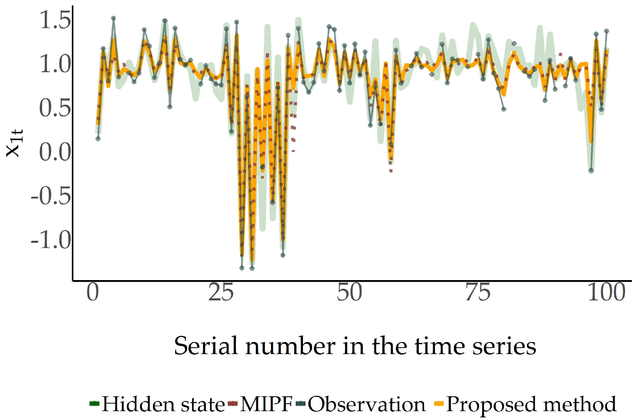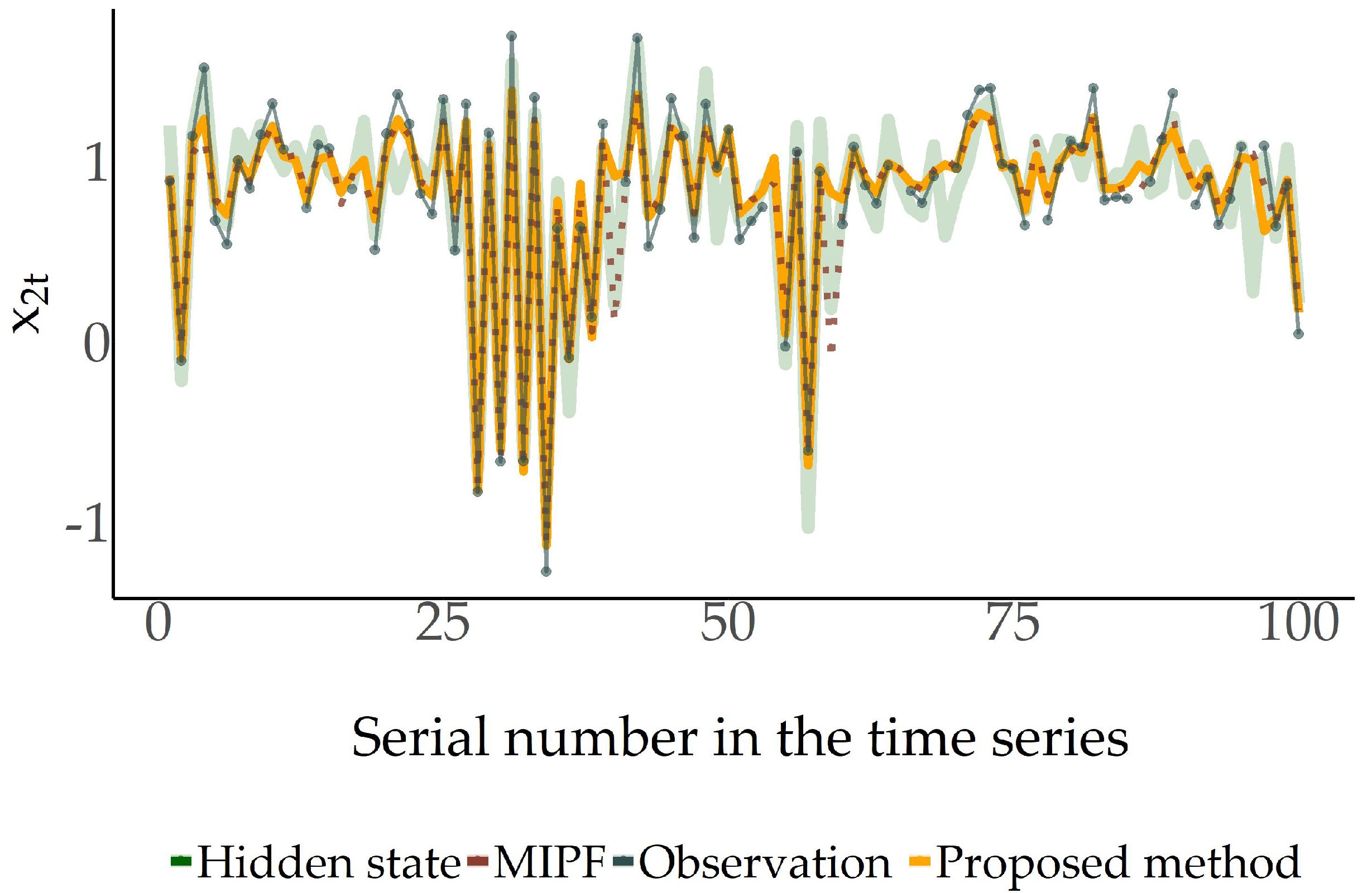In Figure 1 and Figure 2, the performances of the proposed method and MIPF are depicted for the two components of the state process, respectively, for one iteration of each filter. The estimators (weighted means) of the two approaches are close to each other, tracking the hidden vector satisfactorily. Therefore, in this example, the suggested method appears to provide the best option between the available ones in the missing data case.

4.2. Contribution to Impoverishment Prediction

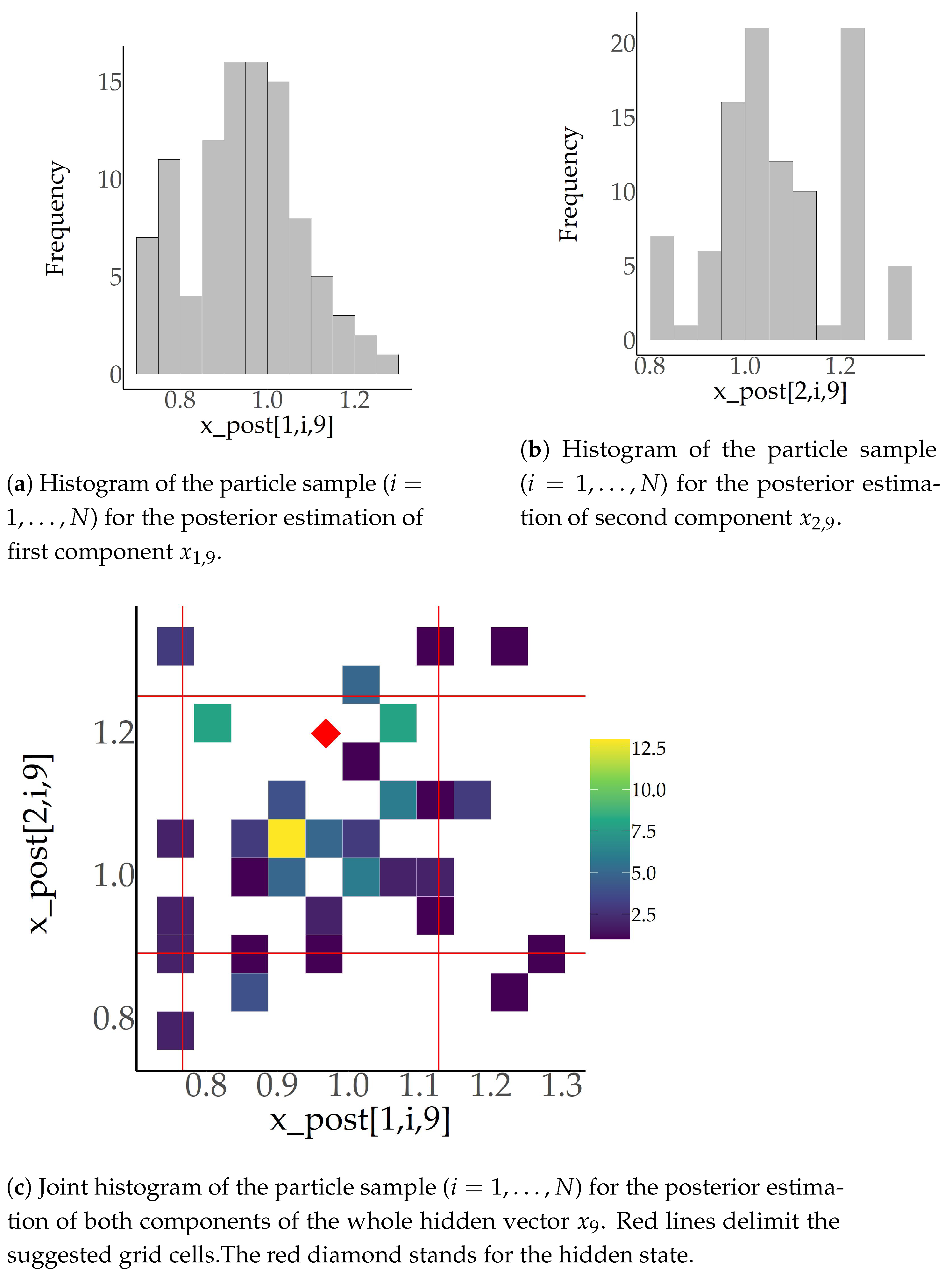
As far as estimation of particle distribution one step ahead is concerned, an application for the transition of the particles from time point $t=9$ to $t=10$ is presented during one implementation of the suggested PF with single imputation for missing values on the available dataset. In the time interval (0,10], only the first component of observation $y_6$ is unavailable. In the end of time step $t=9$, resampling is implemented and the histograms of the particle sets are exhibited in Figure 3. The sample mean of the particles is $m={[m_1=0.947m_2=1.07]}^T$ and the standard deviations of the corresponding components are $s_1=0.126$ and $s_2=0.127$. According to Equation (4) and the given parameters of the problem, the random factor needed to be estimated for every particle at the next time step is

$$z_t^i=A{v}_{t+1}-A{v}_{t+1}^i+u_{t+1}\sim N(0,S_z),S_z=2S_1+S_2=\left(\begin{array}{cc}{\sigma }_z^2& 0\\ 0& {\sigma }_z^2\end{array}\right),$$

where ${\sigma }_z=0.36$. Thus, in both dimensions, the following partitions are considered,

$${\Pi }_j=\{(-\infty ,m_j-{\sigma }_z/2),[m_j-{\sigma }_z/2,m_j+{\sigma }_z/2),[m_j+{\sigma }_z/2,+\infty )\},j=1,2,$$

so that a grid of nine cells is configured over the two dimensions. The frequency table (

Table 2. Frequency table of the particle distribution over the suggested grid at the end of $t=9$.

	2nd Componet	$(-\mathit{\infty },0.89)$	$[0.89,1.25)$	$[1.25,+\mathit{\infty })$
1st Component
$(-\infty ,0.767)$		2	6	3
$[0.767,1.13)$		5	77	1
$[1.13,+\infty )$		1	4	1

) exhibits the particle distribution over the grid.

The selected time period was chosen because there is a considerable number of preceding steps that permits a relatively good adaptation of the particle samples over the hidden states and the samples have not yet collapsed to a tiny neighborhood around a single point (utter impoverishment). This argument is evinced in Figure 3c and Table 2, where the distribution of the particles is presented in connection with the hidden state and the suggested grid. The produced particles are both close to the hidden state, as most of them are less than one standard deviation ${\sigma }_z$ from it, and sparse enough for the existence of particles outside the central cell of the grid. Thus, the condition of the sample during these time points configures a typical example of filter implementation before its collapse. Such time points may be suitable starting points for the introduction of control (which exceeds the limits of this study) as the subject sample is in a good condition concerning both impoverishment and accuracy over hidden variable estimation.

For the next time step, a prior estimation for hidden vector $x_{10}$ is implemented. For the formation of the new grid, the existing particles are moved according to the deterministic part of Equation (9), resulting in $x_{10}(-)={\left[0.9930.984\right]}^T$, the mean of the new particle set. This quantity constitutes a prior point estimator of the hidden state. Thus, the grid of $t=9$ is shifted by $x_{10}(-)-m$ to a new grid, as shown it

Table 3. Frequency table of the particle distribution over the suggested grid at $t=10$ when the particles $x_9^i,i=1,\cdots ,100$, move only according to the deterministic part of Equation (9).

	2nd Componet	$(-\mathit{\infty },0.804)$	$[0.804,1.16)$	$[1.16,+\mathit{\infty })$
1st Component
$(-\infty ,0.813)$		0	0	0
$[0.813,1.17)$		0	100	0
$[1.17,+\infty )$		0	0	0

, the central cell of which is

$$\begin{array}{c}[x_{10}(-)\left[1\right]-0.18,x_{10}(-)\left[1\right]+0.18)\times [x_{10}(-)\left[2\right]-0.18,x_{10}(-)\left[2\right]+0.18)=\hfill \\ \hfill \times [0.804,1.16).\end{array}$$

The movement of all the particles according to the deterministic part of Equation (9) results in the frequency table in Table 3, where it is shown that all the new particles belong to the central cell. Even though the particles are identically distributed, with the addition of the process noise to the particles, the probabilities for particles to move from the central cell to random ones defer from particle to particle, as the particles have different distances form the grid lines initially. This fact is in contrast to the theoretical background of MS, according to which population members have a common transition probability matrix P to move during a time step. For this reason, the probabilities of particles to move to a cell with the addition of the random noise are approximated by the probabilities of the point estimation $x_{10}(-)$ to move to a random cell with the addition of noise. These probabilities (rounded values) are provided in

Table 4. Transition probability table for $x_{10}(-)$ to move with the addition of process noise $v_{10}$.

	2nd Componet	$(-\mathit{\infty },0.804)$	$[0.804,1.16)$	$[1.16,+\mathit{\infty })$
1st Component
$(-\infty ,0.813)$		0.044	0.122	0.044
$[0.813,1.17)$		0.122	0.335	0.122
$[1.17,+\infty )$		0.044	0.122	0.044

. Thus, the expected numbers of particles over the grid cells are

$$N\ast P=100\ast \left(\begin{array}{ccc}0.044& 0.122& 0.044\\ 0.122& 0.335& 0.122\\ 0.044& 0.122& 0.044\end{array}\right)$$

and the expected distribution of the particles over the grid is presented in

Table 5. Frequency table for the expected numbers of the particles over the grid cells after the addition of process noise realizations at $t=10$.

	2nd Componet	$(-\mathit{\infty },0.804)$	$[0.804,1.16)$	$[1.16,+\mathit{\infty })$
1st Component
$(-\infty ,0.813)$		4.4	12.2	4.4
$[0.813,1.17)$		12.2	33.5	12.2
$[1.17,+\infty )$		4.4	12.2	4.4

. Concerning the expected posterior distribution of the particles, the expected observational errors are zero, so that particle weights are expected to remain the same. Thus, no further change is expected in their distribution in cells even if resampling is decided to take place, as all weights are equal after resampling in the previous time step.

Remark 3.

The expected values of observational errors are zero. Nevertheless, the prior estimation of their distribution according to relation (4) and model parameters, where the variances of the errors are presented, evinces the increased uncertainty for them, as ${\sigma }_u^2=0.03$ while ${\sigma }_z^2=0.13$.

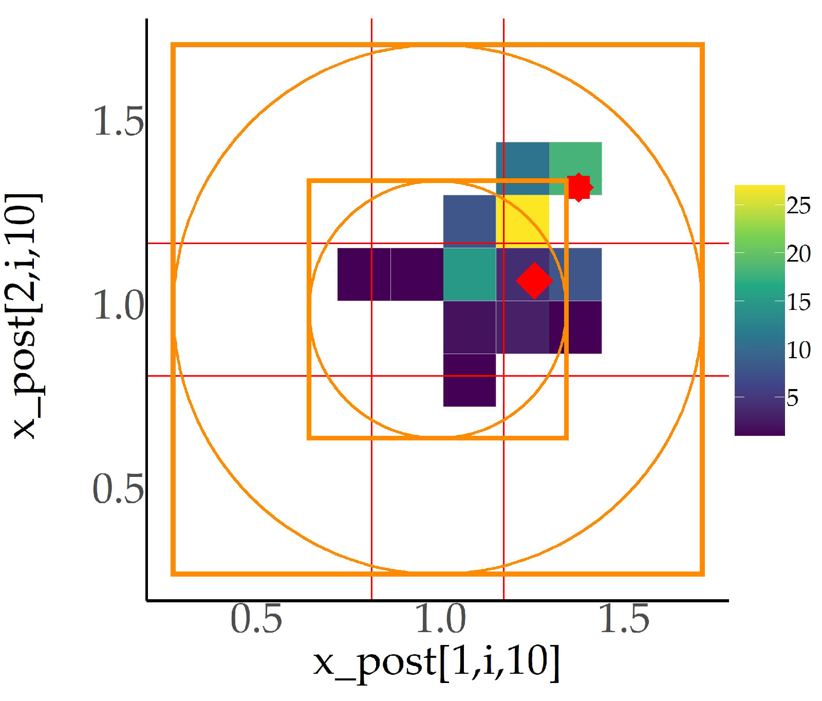
The results of the implementation of PF at time step $t=10$ are also exhibited. Resampling has taken place at this time step as well. The joint histogram of the posterior sample over both dimensions (Figure 4) indicates that the majority of the particles do not belong to the central cell. This fact is reasonable, as the length of the sides of the central cell equals only one standard deviation ${\sigma }_z$, so that prior probabilities for the particles to be placed outside of the central cell at this time point are considerably big according to the Empirical Rule (68-95-99.7) for normal distribution. For the consolidation of these results towards this rule, the orange squares are drawn in Figure 4 for the corresponding areas of the rule to be defined for each separate dimension, while the orange circles are the corresponding standard deviation circles (and not ellipses, generally, as the two components have the same variance ${\sigma }_z^2=0.13$) of the whole vector. Thus, questions on the suitability of the proposed grid structure are raised for future study. Nevertheless, it should be mentioned that a grid with a central cell of double side length would have classified all particles to the central cell during time step $t=9$, rendering further study on the issue meaningless. Additionally, a new grid of nine cells is also constructed around the mean of this posterior particle set, the central cell of which also has length ${\sigma }_z$. The distribution of the particles in the new grid is quoted in

Table 6. Frequency table of the particle distribution over the grid around the mean of the sample in the end of $t=10$.

	2nd Componet	$(-\mathit{\infty },1.01)$	$[1.01,1.37)$	$[1.37,+\mathit{\infty })$
1st Component
$(-\infty ,1.06)$		1	3	0
$[1.06,1.42)$		6	90	0
$[1.42,+\infty )$		0	0	0

. In comparison with Table 2, it seems that the number of particles in the central cell is increased in Table 6.

Remark 4.

In the present example, the transitions of the particles according to the deterministic function led all particles to a single cell (Table 3), so that the result of the addition of process noise was handled as a result of a multinomial trial. In the case that the deterministic function leads the particles to more than one cell, then it is suggested that different means be found for each cell as well as corresponding transition probabilities, so that the final result can be considered the sum of results of multinomial trials for the transitions to every cell.

5. Discussion and Conclusions

In this study, single substitution (in contrast to MIPF) of observational errors is proposed for missing data cases, when PF is implemented and MAR assumption is adopted. This method is a single imputation procedure. Acuña et al. [23] argued against single imputation, as it is rather simplistic and it cannot attribute to a single value the distributional characteristics that can be approached and described by a sample of multiple imputation. Nevertheless, the primary target of the proposed technique is the minimization of the computational cost that is added to the initial PF algorithm, in the case of missing data. For this purpose, interventions in the PF algorithm are slight. Moreover, in the provided simulation, the suggested method outperforms the multiple imputation approach even for a considerable number of imputations, whereas Acuña et al. [23] noticed that MIPF with $n=3,4,5$ imputations produces very satisfactory results, according to the approximation of multiple imputation estimator of efficiency provided by Rubin [29]. As a result, in this example, estimation of observational errors performs better with respect to both the computational time it requires and the precision it achieves. Besides, knowledge on the distribution of the observational errors contributes to the quantification possibility of the uncertainty over the point estimations. Thus, the suggested method takes advantage of the low computational cost of the single imputation option, while the study of more general distributional characteristics of the observational noise can also be taken into account at the same time (see Remark 3).

The contribution of such a method in order to cope with impoverishment problems is also worth mentioning. This method permits the estimation of observational errors and their corresponding weights one time step forward. The evolution of weight distribution has not been a priori estimated for multiple time steps yet, to the best of the authors’ knowledge, but this is feasible at least for one step ahead. As the weights of the next step can be estimated, the probabilities that a particle will be chosen at the resampling step can also be estimated. As explained in Section 3.1, the assessment of weight distribution for the forthcoming time steps could be very interesting, as far as it is connected with impoverishment issues. Concerning future perspectives over this issue, the study of impoverishment problems can be implemented with the use of input control [12], in order for the impoverishment to be controlled; laws of large numbers [30], as MC approximation employs large samples; state capacity restrictions [31]; for the existence of a population limit at every grid cell; literature on the evolution of attainable structures [32]; the evolution of the distribution of particles [33] or of the corresponding moments [34] in the direction of HMSs and NHMSs; and for the estimation of the future behaviour of the sample, possibly reaching continuous-time models [35]. Research on automatic optimal control [36] could be combined with the suggested methodology, possibly leading to interesting joint applications of PF [37] along with artificial intelligence [38]. The performance of the method could also be tested when data are missing for longer time periods [39], while more sophisticated grid structures could also be examined [18]. Correspondingly, in a broader sense, the main idea of the proposed method could be implemented in the errors-in-variables signal processing for missing data cases [40], or it could be involved in more complex models that require MC simulation for the prior estimation of variables [41].

References

1. Gordon, N.; Salmond, D.; Smith, A. Novel approach to nonlinear/non-Gaussian Bayesian state estimation. IEE Proc. Radar Signal Process. 1993, 140, 107. [Google Scholar] [CrossRef] [Green Version]
2. Metropolis, N.; Ulam, S. The Monte Carlo Method. J. Am. Stat. Assoc. 1949. [Google Scholar] [CrossRef]
3. Wang, X.; Li, T.; Sun, S.; Corchado, J.M. A Survey of Recent Advances in Particle Filters and Remaining Challenges for Multitarget Tracking. Sensors 2017, 17, 2707. [Google Scholar] [CrossRef] [Green Version]
4. Degen, C.; Govaers, F.; Koch, W. Track maintenance using the SMC-intensity filter. In Proceedings of the 2012 Workshop on Sensor Data Fusion: Trends, Solutions, Applications (SDF), Bonn, Germany, 4–6 September 2012; pp. 7–12. [Google Scholar] [CrossRef]
5. Dempster, A.P.; Laird, N.M.; Rubin, D.B. Maximum Likelihood from Incomplete Data Via the EM Algorithm. J. R. Stat. Soc. Ser. B (Methodol.) 1977, 39, 1–22. [Google Scholar] [CrossRef]
6. Metropolis, N.; Rosenbluth, A.W.; Rosenbluth, M.N.; Teller, A.H.; Teller, E. Equation of State Calculations by Fast Computing Machines. J. Chem. Phys. 1953, 21, 1087–1092. [Google Scholar] [CrossRef] [Green Version]
7. Gopaluni, R.B. A particle filter approach to identification of nonlinear processes under missing observations. Can. J. Chem. Eng. 2008, 86, 1081–1092. [Google Scholar] [CrossRef]
8. Housfater, A.S.; Zhang, X.P.; Zhou, Y. Nonlinear fusion of multiple sensors with missing data. In Proceedings of the 2006 IEEE International Conference on Acoustics Speech and Signal Processing Proceedings, Toulouse, France, 14–19 May 2006. [Google Scholar] [CrossRef] [Green Version]
9. Xu, L.; Ma, K.; Li, W.; Liu, Y.; Alsaadi, F.E. Particle filtering for networked nonlinear systems subject to random one-step sensor delay and missing measurements. Neurocomputing 2018, 275, 2162–2169. [Google Scholar] [CrossRef]
10. Rubin, D.B. Inference and Missing Data. Biometrika 1976, 63, 581. [Google Scholar] [CrossRef]
11. Vassiliou, P.C.G. Asymptotic behavior of Markov systems. J. Appl. Probab. 1982, 19, 851–857. [Google Scholar] [CrossRef]
12. Vassilliou, P.C.G.; Tsantas, N. Stochastic control in non- homogeneous markov systems. Int. J. Comput. Math. 1984, 16, 139–155. [Google Scholar] [CrossRef]
13. Li, T.; Sun, S.; Sattar, T.P.; Corchado, J.M. Fight sample degeneracy and impoverishment in particle filters: A review of intelligent approaches. Expert Syst. Appl. 2014, 41, 3944–3954. [Google Scholar] [CrossRef] [Green Version]
14. Lykou, R.; Tsaklidis, G. A priori estimation methodology on observation errors of a state space model with linear observation equation using Particle Filtering. In Proceedings of the 6th Stochastic Modeling Techniques and Data Analysis International Conference; Skiadas, C.H., Ed.; Barcelona, Spain, 2–5 June 2020, pp. 333–341.
15. Liu, J.S. Monte Carlo Strategies in Scientific Computing; Springer Series in Statistics; Springer: New York, NY, USA, 2004. [Google Scholar] [CrossRef]
16. Lykou, R.; Tsaklidis, G. Prior estimation of observational errors of Particle Filter. In Proceedings of the 32nd Panhellenic Statistics Conference, Ioannina, Greece, 30 May–1 June 2019; pp. 195–204. (In Greek). [Google Scholar]
17. Bartholomew, D.J. A Multi-Stage Renewal Process. J. R. Stat. Soc. Ser. B (Methodol.) 1963, 25, 150–168. [Google Scholar] [CrossRef]
18. Li, T.; Sattar, T.P.; Sun, S. Deterministic resampling: Unbiased sampling to avoid sample impoverishment in particle filters. Signal Process. 2012, 92, 1637–1645. [Google Scholar] [CrossRef]
19. Bartholomew, D.J. Stochastic Models for Social Processes, 3rd ed.; Wiley: New York, NY, USA, 1982. [Google Scholar]
20. Beaulieu, N. On the generalized multinomial distribution, optimal multinomial detectors, and generalized weighted partial decision detectors. IEEE Trans. Commun. 1991, 39, 193–194. [Google Scholar] [CrossRef]
21. Poisson, S.D. Recherches sur la Probabilité des Jugements en Matière Criminelle et en Matière Civile; Bachelier: Paris, France, 1837. [Google Scholar]
22. Vassiliou, P.C.G.; Georgiou, A.C.; Tsantas, N. Control of Asymptotic Variability in Non-Homogeneous Markov Systems. J. Appl. Probab. 1990, 27, 756–766. [Google Scholar] [CrossRef]
23. Acuña, D.E.; Orchard, M.E.; Silva, J.F.; Pérez, A. Multiple-imputation-particle-filtering for uncertainty characterization in battery state-of-charge estimation problems with missing measurement data: Performance analysis and impact on prognostic algorithms. Int. J. Progn. Health Manag. 2015, 6, 1–12. [Google Scholar]
24. R Core Team. R: A Language and Environment for Statistical Computing. 2014. Available online: https://www.gbif.org/tool/81287/r-a-language-and-environment-for-statistical-computing (accessed on 20 June 2021).
25. Genz, A.; Bretz, F.; Miwa, T.; Mi, X.; Leisch, F.; Scheipl, F.; Hothorn, T. {mvtnorm}: Multivariate Normal and t Distributions. 2020. Available online: http://mvtnorm.r-forge.r-project.org/ (accessed on 20 June 2021).
26. Genz, A.; Bretz, F. Computation of Multivariate Normal and t Probabilities; Lecture Notes in Statistics; Springer: Heidelberg, Germany, 2009. [Google Scholar]
27. Wickham, H. ggplot2: Elegant Graphics for Data Analysis; Springer: New York, NY, USA, 2016. [Google Scholar]
28. Pedersen, T.L. ggforce: Accelerating ’ggplot2’, R package version 0.3.3; 2021. Available online: https://cran.r-project.org/web/packages/ggforce/index.html (accessed on 20 June 2021).
29. Rubin, D.B. (Ed.) Multiple Imputation for Nonresponse in Surveys; Wiley Series in Probability and Statistics; John Wiley & Sons, Inc.: Hoboken, NJ, USA, 1987. [Google Scholar] [CrossRef]
30. Vassiliou, P.C. Laws of Large Numbers for Non-Homogeneous Markov Systems. Methodol. Comput. Appl. Probab. 2020, 22, 1631–1658. [Google Scholar] [CrossRef] [Green Version]
31. Vasiliadis, G.; Tsaklidis, G. On the Distributions of the State Sizes of the Closed Discrete-Time Homogeneous Markov System with Finite State Capacities (HMS/c). Markov Process. Relat. Fields 2011, 17, 91–118. [Google Scholar]
32. Tsaklidis, G.M. The evolution of the attainable structures of a homogeneous Markov system by fixed size. J. Appl. Probab. 1994, 31, 348–361. [Google Scholar] [CrossRef]
33. Kipouridis, I.; Tsaklidis, G. The size order of the state vector of discrete-time homogeneous Markov systems. J. Appl. Probab. 2001, 38, 357–368. [Google Scholar] [CrossRef]
34. Vasiliadis, G.; Tsaklidis, G. On the moments of the state sizes of the discrete time homogeneous Markov system with a finite state capacity. In Recent Advances in Stochastic Modeling and Data Analysis; Skiadas, C.H., Ed.; 2007; pp. 190–197. [Google Scholar] [CrossRef]
35. Vasiliadis, G.; Tsaklidis, G. On the Distributions of the State Sizes of Closed Continuous Time Homogeneous Markov Systems. Methodol. Comput. Appl. Probab. 2009, 11, 561–582. [Google Scholar] [CrossRef]
36. Sands, T. Optimization Provenance of Whiplash Compensation for Flexible Space Robotics. Aerospace 2019, 6, 93. [Google Scholar] [CrossRef] [Green Version]
37. Bachmann, A.; Williams, S.B. Outlier handling when using particle filters in terrain-aided navigation. IFAC Proc. Vol. 2004, 37, 358–363. [Google Scholar] [CrossRef]
38. Sands, T. Development of Deterministic Artificial Intelligence for Unmanned Underwater Vehicles (UUV). J. Mar. Sci. Eng. 2020, 8, 578. [Google Scholar] [CrossRef]
39. Orchard, M.E.; Cerda, M.A.; Olivares, B.E.; Silva, J.F. Sequential monte carlo methods for discharge time prognosis in lithium-ion batteries. Int. J. Progn. Health Manag. 2012, 3, 90–101. [Google Scholar]
40. Maciak, M.; Pešta, M.; Peštová, B. Changepoint in dependent and non-stationary panels. Stat. Pap. 2020, 61, 1385–1407. [Google Scholar] [CrossRef]
41. Maciak, M.; Okhrin, O.; Pešta, M. Infinitely stochastic micro reserving. Insur. Math. Econ. 2021, 100, 30–58. [Google Scholar] [CrossRef]
Figure 1. Time-series of the hidden values, the observations, and the corresponding point estimations of the proposed method and MIPF imputations for the first component x 1 , t of the state process.
Mathematics 09 01445 g001
Figure 2. Time-series of the hidden values, the observations, and the corresponding point estimations of the proposed method and MIPF imputations for the second component x 2 , t of the state process.
Mathematics 09 01445 g002
Figure 3. Histograms of particle samples for the posterior estimation of hidden variable x 9 .
Mathematics 09 01445 g003
Figure 4. Joint histogram of the particle sample ( i = 1 , , N ) for the posterior estimation of both components of the whole hidden vector x 10 . Red lines delimit the suggested grid cells of Table 3. The red diamond stands for the hidden state. The red star stands for the observation at this time point. The sides of the two squares are correspondingly one and two standard deviations σ z from the center of the diagram. The circles are inscribed in the corresponding squares.
Mathematics 09 01445 g004