1. Introduction
Spatial econometric models are mainly used to deal with spatial dependent data in applications. Spatial dependence across sectional units may concern a spatial autocorrelation in a dependent variable or disturbance term. The first form of dependence is usually defined by a spatial autoregressive (SAR) model and another by a spatial error model (SEM). In fact, both spatial dependencies may be reflected in a spatial autoregressive model with autoregressive disturbances (SARAR). These models were first introduced by Cliff and Ord [
1], which have aroused wide concern, see, e.g., the research by Kelejian and Prucha [
2], Lee [
3], Arraiz et al. [
4], and the books by Anselin [
5] and Cressie [
6].
In practice, explanatory variables are needed to be chosen from a number of variables during the initial data analysis. How to select significant variables to keep in the final model becomes very important for further analysis. Therefore, variable selection has received increasing attention in statistical modeling and inference. However, the study of variable selection in spatial econometric models is not as sufficient as that in classical linear models due to the complexity caused by spatial dependence. The main goal of our analysis is to fill some gaps in this area to a certain degree. We mainly focus on a variable selection method for the SARAR model based on a penalized quasi-likelihood method and investigate its oracle property. Furthermore, a feasible algorithm is given for realizing these procedures.
The methods of variable selection for classical linear models have been developed rapidly since the Akaike information criterion (AIC) was proposed by Akaike [
7]. Then, similar methods based on the information criterion have progressed remarkably, such as the Bayesian information criterion (BIC) [
8], risk inflation criterion (RIC) [
9], etc. Using these criteria, the best subset selection became the standard method to select covariants for a long time. Although they are practically useful, the common drawback is the lack of stability and incorporating stochastic errors from each stage of variable selection as noted by Liang and Li [
10]. Moreover, it may require a comparison of all possible submodels. This is a combinational problem with NP-complexity [
11]. In order to overcome these drawbacks, penalized methods of variable selection have been proposed in recent years, including least absolute shrinkage and selection operator (LASSO) [
12], smoothly clipped absolute deviation (SCAD) penalty [
13], elastic-net (ENet) [
14], adaptive LASSO [
15], minimax concave penalty (MCP) [
16], and so on. These methods can select significant variables and estimate unknown parameters simultaneously. Fan and Li [
13] established the oracle property in the sense that the penalized estimator behaves the same as the ordinary least squares estimator as we know the true linear model, which can be used to assess the efficiency of the penalized estimator. In the Bayesian framework, some developments include Mitchell and Beauchamp [
17], Raftery et al. [
18], Jiang [
19], etc. Other related methods can be found in Chen et al. [
20] and Steel [
21].
Along with the rapid development of the geographic information system (GIS), variable selection for the spatial econometric models has become a new concern in the last 10 years or so. Based on the Bayesian idea, LeSage and Parent [
22] developed the Bayesian model averaging (BMA) technique for the SAR model and SEM. Some extension works include LeSage and Fischer [
23] and Cuaresma et al. [
24,
25]. In order to avoid the complex calculation of marginal likelihoods in BMA, Piribauer [
26] used stochastic search variable selection (SSVS) prior to deal with the identification of the SAR model. Generally, it is challenging to extend the penalized methods to data that are dependent either over time or across space, as variable selection involves not only regression coefficients but also auto-correlation coefficients [
27]. In recent years, Liu et al. [
28] gave an efficient variable selection procedure for the SAR model and obtained the large sample properties by a penalized quasi-likelihood method. Using SCAD penalty and instrumental variable, Xie et al. [
29] considered variable selection in the SAR model with a diverging number of parameters. They showed that the SCAD penalty in the SAR model for variable selection also has a nice oracle property as in the classical linear model.
High dimensional spatial data may lead to complex and multiple spatial dependencies. However, the existing methods are constrained by dimension and spatial heterogeneity, which brings great challenges to the application of traditional spatial econometric models. Although the technology of dimension reduction by eliminating redundant information through variable selection in classical linear models is being gradually developed and the research on variable selection in spatial lag models has been completed, it is still difficult to effectively solve the problem of variable selection with spatial heterogeneity in error terms. The SARAR model has both a dependent variable spatial effect and spatial error term, it can reflect spatial effect information and describe spatial heterogeneity relatively comprehensively. Moreover, once the spatial effect of error is ignored, it will lead to model recognition errors, reduce the estimation error and prediction accuracy, and bring concerns to the application research. In light of the above considerations and the excellent performance of penalized methods, we studied the variable selection of spatial cross-section data based on the SARAR model. The main contributions are as follows: (1) For high-dimensional spatial heterogeneous data, a penalty quasi-likelihood method is proposed to solve the problem of dimensionality reduction of explanatory variables and the identification of two kinds of spatial effects. (2) Using the idea of step-by-step transformation, a new iterative numerical algorithm is proposed to avoid the influence of spatial heterogeneity. (3) Simulation and case analysis will help practitioners in related fields to use reasonably. (4) The proposed method can provide a useful reference for the study of variable selection in semi-parametric and nonparametric spatial regression models.
The remainder of this paper is as follows.
Section 2 presents a penalized quasi-likelihood method in the SARAR model.
Section 3 introduces a feasible algorithm to complete a variable selection procedure.
Section 4 provides a Monte Carlo study to investigate the finite sample performance.
Section 5 illustrates the proposed method through an application of the Boston housing data. Summary and discussion is stated in
Section 6.
Appendix A and
Appendix B contain some assumptions and proofs of theorems.
2. Model and Variable Selection
2.1. The SARAR Model
The SARAR model can be specified as:
where
denotes an
vector of observations on the dependent variable,
is an
matrix of observations on
k exogenous explanatory variables,
and
are known
spatial weight matrices,
is a
k-dimensional parameter vector of regression coefficients,
and
are scalar spatial autoregressive coefficients with
and
,
is an
vector of regression disturbances, both
and
are the spatial lag term and spatial error lag term respectively, and
is an
n-dimensional vector of i.i.d. innovations with zero mean and finite variance
. Note that this model is also known as the Cliff–Ord model or the SARAR(1,1) model. The SAR model and SEM are corresponding to
and
, respectively.
Let
be the true value of
, and
. Denote
,
,
, where
. According to the idea of quasi-maximum likelihood estimation [
3], we can write the log-quasi-likelihood function of the model (1) as
where
is the quasi-likelihood function of the model (1).
2.2. Penalized Method
The spatial econometric research has shown that it is inappropriate to use the the ordinary least squares estimation (OLS) method directly for SAR models. In the case of the SARAR model, the OLS estimators of the spatial autoregressive coefficients are biased and inconsistent. Therefore, the penalized least squared method can not be directly used for variable selection in this model. Considering a good performance of the quasi-maximum likelihood estimation in the SARAR model, the penalized quasi-likelihood method deserves priority. We start with a penalized quasi-likelihood function for the model (1) defined as:
where
is the SCAD penalty function defined by Fan and Li [
13] as:
For comparison, we also introduce the following two popular penalty functions.
HARD thresholding penalty function:
In fact, the
penalty function corresponds to the LASSO [
12]. The AIC and BIC correspond to the penalty functions
and
respectively because
gives the size of the selected submodel.
In the classical linear models, Fan and Li [
13] proposed that a perfect variable selection method should possess the following three properties:
- (1)
Unbiasedness: The resulting estimator is nearly unbiased when the true unknown parameter is large to avoid unnecessary modeling bias;
- (2)
Sparsity: The resulting estimator automatically sets small estimated coefficients to zero to reduce model complexity;
- (3)
Continuity: The resulting estimator is continuous in data to avoid instability in the model prediction.
Under some regular conditions, they showed that variable selection via the SCAD penalty function possesses above properties, but the other penalty functions proposed above may not satisfy the three properties simultaneously. Related references can be seen in Fan and Li [
13], and Wang and Zhu [
30] for more information.
2.3. Main Results
Note that it may be chaotic in the arrangement of the original non-zero elements of . Re-labeling can put the non-zero elements in the front together and separate them from the zero elements, which is convenient for the concise expression of the theorems and proofs. Therefore, denote , where we assume that is a vector containing s nonzero elements and is a -dimensional zero vector. is the penalized quasi-likelihood estimator of . The theorems stated below give some satisfactory properties of a large sample.
Theorem 1. Suppose that and the assumptions in Appendix A hold. Then there is a local minimizer of such that:where For the SCAD penalty function, the exists at any non-zero point by choosing a proper . Theorem 1 shows that there is a local minimizer of which is a consistent penalized quasi-likelihood estimator by choosing appropriate regularization parameter .
Theorem 2. Suppose that the assumptions in Appendix A hold, satisfies . Then with probability approaching one, the consistent local minimizer in Theorem 1 must satisfy: Theorem 2 shows that the proposed method can identify the SAR model (
), SEM (
), SARAR model (
), select explanatory variables and estimate unknown parameters simultaneously. Similar to the analysis of Fan and Li [
13], if
as
, then
for both SCAD and HARD thresholding penalty functions. Moreover, we obtain that
and
as
Thus, under regular conditions, the responding oracle property of the penalized quasi-likelihood estimators can be obtained. That is, the penalized quasi-likelihood estimators perform asymptotically as well as the ordinary quasi-likelihood estimators for nonzero parameters when knowing the correct submodel. However, for the LASSO penalty function, some conditions in Theorem 2 can not be satisfied.
3. Algorithm Design and Implementation
In this section, we consider the implementation of the proposed procedures. Since the penalized quasi-likelihood function
is nonconcave, it is challenging to get the global optimum solution. The study by Liu et al. [
28] proposed: The existing algorithms, such as local quadratic approximation (LQA) algorithm [
13] and local linear approximation (LLA) algorithm [
31], can not be used directly to the SAR model. Similarly, those algorithms also do not give the correct minimizer of
for the SARAR model. Hence, we design the following iterative algorithm.
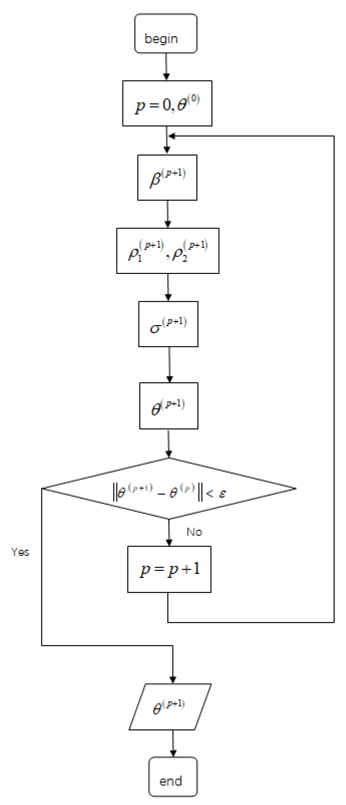
Iterate (5) to (7) until the successive value satisfies , where and is a given tolerance value. In the following simulation, we let be . Denote the final estimate of as , then .
In (4), the initial value of
is the quasi-maximum likelihood estimate based on the log-quasi-likelihood function of the model (1). In (5), we note that if both autoregressive coefficients
and
are known in the SARAR model (1), then we can transform it as the following linear model
where
,
. Therefore, the LQA algorithm can be used to complete this step as in the classical linear models. In (6), the optimization problem of bivariate functions can be solved by the Nelder–Mead method [
32]. In (7), by using the partial derivative, the unique minimum point is:
where
Figure 1 presents a flowchart of the proposed algorithm.
To implement the above algorithm, the tuning parameters need to be chosen. For the SCAD penalty function, we set
as recommended by Fan and Li [
13]. Moreover, it is desirable to select a proper data-driven method to estimate all tuning parameters
. Wang et al. [
33] proved that the optimal tuning parameter in the SCAD penalty can be determined by BIC for the linear regression models. Thus, we can select
by the following Bayesian information criterion:
where
Then
is set to be
.
In fact, minimizing the BIC over a -dimensional space is an unduly onerous task for a large k. To save computation time, one may use the same tuning parameter for all penalty functions. However, the experiments, though not given for saving space, show that the spatial regression coefficient is easy to compress to 0 even if the sample size is medium. Intuitively, we should use different tuning parameters for spatial regression coefficients and regression coefficients because the range of are known before estimation, but the range of are not. Thus, we set , and to optimize the results. It should be pointed out that we can prove the consistency of the BIC criterion under more stringent conditions, such as the bounded derivative of the quasi-likelihood function and . However, it is very difficult to prove the consistency under some mild conditions and will be left for further study.
4. Numerical Simulation
In this section, we conduct some Monte Carlo experiments to evaluate the finite sample performance of the proposed variable selection method in the SARAR model using R codes.
4.1. Simulation Sampling
The sample data is generated by model (1). We consider eight explanatory variables following an 8-dimensional normal distribution with zero mean and covariance matrix
, where
. The spatial autoregressive coefficients are set to be
and
For simplicity, let
, where
, ⊗ is the Kronecker product, and
is an
m-dimensional column vector of ones [
3,
34], which is called the Case spatial weight matrix. To observe the influence of different spatial weight matrices, the Rook spatial weight matrix is introduced, in which
is set to be 1 when the regions share a common boundary and set to be 0 for other cases. For the Case spatial weight matrix, we take
and different values of
R, where
, then corresponding sample sizes are
. For the Rook spatial weight matrix, we use the grid square area to generate it according to whether the edges are adjacent. To ensure that the region is square, the value of
n is the square of the integer value and
. The regression coefficients are assumed to be
. The innovation
follows a normal distribution with mean 0 and variance
.
4.2. Simulation Results
For each case, we do 100 repetitions. The average number of zero coefficients which are correctly identified is denoted as “C”. The label “I” indicates the average number of non-zero coefficients incorrectly shrunk to zero. To measure the estimation accuracy of
, we compare the estimation accuracy using the medians of squared error (SE) as in Liang and Li [
10], which is defined as:
where
is the estimate of
In
Table 1,
Table 2 and
Table 3, Oracle implies the results of variable selection knowing zero parameters. Moreover, other penalty functions, such as HARD and LASSO, are introduced in the penalized quasi-likelihood function for comparison.
Table 1,
Table 2 and
Table 3 clearly show that there are similar performances for variable selection under both different spatial weight matrices. In other words, the proposed method is not sensitive to the change of the spatial weight matrix. As we expected, all penalty functions can reduce their mSE (the median of SE) and give close results of Oracle with the increase of sample size. In most cases, the SCAD penalty produces the lowest mSE, the HARD penalty has a little bigger than the SCAD penalty, and the LASSO penalty produces the largest mSE. Moreover, if there are spatial effects for both the spatial lag term and the spatial error lag term (
and
), the mSE is often relatively large; if only one of the spatial lag term and the spatial error lag term is related to the spatial effect (
, and
), the value of the mSE is usually smaller, especially when there is no spatial effect (
and
). However, like most of the existing results of variable selection, the mSE will be less accurate in all cases if the variance
of the innovation becomes large. In terms of C and I, we can see that the average number of correctly identifying zero-valued coefficients approaches the true value and the average number of incorrectly identifying zero-valued coefficients approaches 0 as the sample size
n increases. These simulation results accord with the theoretical analysis. The SCAD and HARD penalties have good performance about C, there is little difference between them in most cases. They can converge rapidly to the real number of 0 except a LASSO penalty with a low convergence rate, which may imply that both SCAD and HARD tend to give smaller models than LASSO. In the case of small samples, the LASSO penalty has the lowest value of the I in most cases. However, their differences quickly disappear in large samples for all penalties. These results are similar to those obtained by Fan and Li [
13]. It is worth noting that when
is small, it is easy to compress to 0, and then produce a larger error rate I in the setting of small samples.
Table 4 shows the results of ignoring spatial effects by the LQA algorithm [
13] under the same context as in
Table 1. In terms of I, when there are two spatial effects (
and
), the number of incorrect zero in
Table 1 is much lower than those in
Table 4. When only one spatial effect exists (
, or
), the number of incorrect zero in
Table 4 decreases slightly compared to the first case and is also larger than that in
Table 1. When there is no spatial effect (
and
), the results of our algorithm are close to that of the LQA algorithm. Meanwhile, turning attention to the C, our algorithm can identify more true zeros than the LQA algorithm as long as the spatial effect exists (
). Although we are surprised to find that the value of C and I under the LQA algorithm seem to be getting close to the correct values with slow speed as the sample size increases for the SCAD and HARD penalties, the mSE reflected the estimation errors of their parameters are large and outrageous. This is in line with our intuition: Ignoring both spatial effects, the LQA algorithm is implemented on the wrong model and easily leads to a large estimated deviation. Moreover, the LQA algorithm is affected by the initial estimation. In simulation, the initial estimation is the quasi-maximum likelihood estimation, which is equal to the least square estimation (including the observation value of dependent variable
). If the strong spatial effect about
is ignored, the observation value of the dependent variable will deviate from the requirement of unbiased estimation seriously, which will lead to a great deviation of the initial estimation. With the influence of iteration, the accumulated error of final estimation will be extraordinary. However, when the spatial effects disappear, we can see that both algorithms have similar good performances, which indicates that no matter whether there are spatial effects, the proposed algorithm still has a satisfactory performance in a finite sample.
Considering the complexity of the asymptotic covariance matrix of , we use the traditional bootstrap method in which the sample size of the resampled observations is 100 to obtain the standard deviations of parameter estimates. The parameter vector is estimated by our algorithm. SD indicates the median absolute deviation of 100 estimated coefficients in the 100 simulations, which can be regarded as an estimate of the true standard deviation of . Using the bootstrap, we calculate a median of estimated standard deviations, denoted as SDm, and estimate its standard deviation by median absolute deviation, denoted as SDmad.
Table 5 provides the numerical simulation results of nonzero coefficients under
,
,
, and
with the Case spatial weight matrix. The simulation results show that the bootstrap estimated standard deviation becomes increasingly accurate when sample size
n increases. In most cases, the SD, SDm, and SDmad obtained by the SCAD and HARD penalties are smaller than that obtained by the LASSO penalty, which shows that the LASSO penalty does not appear to be as stable as the SCAD and HARD penalties. Furthermore, when the
increases and is away from 1, the estimation of the standard deviation will be less accurate although the results are not presented. In one world, the LASSO penalty generally lags behind the SCAD and HARD penalties concerning the accuracy of estimates. For saving space, the other cases, such as
, or
, have similar results and are omitted.
5. Data Example
Now, we consider a real example for the application and performance of the proposed variable selection method in the SARAR model.
5.1. The Sample Data
We consider the Boston housing data set which was originally given by Harrison and Rubinfeld [
35] and has been used by many authors, for example, Pace and Gilley [
36,
37], and so on. The data set contains 506 census tracts with 14 nonconstant independent variables. It can be found in the spdep library of R. Similar to the analysis of Harrison and Rubinfeld [
35], the dependent variable is set to be
and the explanatory variables are assumed as
, AGE,
,
, TAX, PTRATIO,
,
, CRIM, ZN, INDUS, CHAS, and
.
Table 6 gives the interpretation of all abbreviated variables. For subsequent analysis, the data are centralized and standardized. The spatial weight matrix is constructed with rook contiguity: The weight is 1 if two different areas share a common boundary, and 0 otherwise. Then the matrix is row-normalized as is usually carried out in practice.
5.2. Spatial Dependence Test
In spatial data analysis, the Moran’s I statistic (Moran I) is usually used to test spatial dependence.
Table 7 shows the value of the Moran’s I in the Boston housing data. It is 0.7644 with a
p-value
, which implies that the MEDV has a strong spatial correlation. It is well known that the Moran’s I reflects the degree of spatial autocorrelation and can not effectively identify specific spatial autoregressive models due to the existence of different spatial correlations. Fortunately, the popular Lagrange multiplier diagnostics can help us to complete this specification for several different spatial autoregressive models. This test method avoids the optimization of the nonlinear function and is easy to implement. Using the spdep package in R, we can obtain the desired results for identification. From
Table 7, it is obvious to see that the
p-value in each case is very small, which implies that the Boston housing data can be modeled by spatial models. However, the values of test statistics and p-values suggest that the SARAR model is the best choice among these spatial models to fit the Boston housing data. Moreover, previous studies have used multiple hypothesis tests to judge spatial effects and select explanatory variables, and then determine the model. It is difficult to prove the relevant theoretical properties. Based on the proposed variable selection method, the SARAR model can not only be used to identify different spatial effects and select explanatory variables simultaneously, but also has a good theoretical guarantee. Therefore, we will use the SARAR model for variable selection in this data.
5.3. Model Selection and Estimation
Under a SARAR model, the results are reported in
Table 8, where the quasi-maximum likelihood estimate (QMLE) and penalized quasi-likelihood estimate (PQLE) via the SCAD, HARD, and LASSO penalties are listed to assess the performance of variable selection.
The QMLE demonstrates that there are four variables that show a relatively small impact on the MEDV, including ZN, INDUS, CHAS, and AGE. These variables in other studies also show a small effect on the MEDV, such as Harrison and Rubinfeld [
35], Pace and Gilley [
36], and so on. Moreover, variables with positive effects include ZN, INDUS, RM
,
,
, while others have negative effects. As we expected, the parameter estimates obtained by the penalized method are close to the QMLE, and both nonzero estimates keep the same sign. Moreover, the four insignificant variables (ZN, INDUS, CHAS, and AGE) are penalized to zero under different penalty functions. Therefore, these penalties produce the same selection results in this setting. However, BIC in
Table 8 shows that the SCAD and HARD penalties are preferable to the LASSO penalty. Interestingly, although the spatial correlation coefficients
and
are also penalized by different penalty functions, they do not shrink to zero and have similar results with the QMLE. From the perspective of model specification, we can say that the penalty method recognizes the spatial autoregressive relationship.
For comparison, the Boston housing data is also fitted by a classical linear regression model and the related results are presented in
Table 9. The QMLE shows that there are three unimportant variables, including ZN, INDUS, and AGE. Moreover, variables with positive effects include ZN, INDUS, CHAS, RM
, AGE,
,
, while others have negative effects. In addition, all penalties also produce the same selection results in this model. According to the QMLE, these penalties can also select important variables and shrink unimportant variables to zero. Based on the BIC, the SCAD and HARD penalties also outperform the LASSO penalty in this setting.
Although both models have similar selection results, the differences between them are quite obvious. For the QMLE, the estimated coefficient of AGE is negative in the SARAR model, a plausible result, but it is positive in the linear model, which seems implausible. For the PQLE, it is easy to see that the CHAS disappears in the SARAR model while it is relatively important in the linear model. Furthermore, the meaning of the parameter estimation in these two models is also distinctly different. The interpretation of parameter estimates in the SARAR model will become richer and more complicated than that in the linear model because of the spatial autocorrelation [
38]. As we expected, the BIC for the SARAR model is far less than that for the classical linear model, which indicates that the SARAR model has a better fitting effect than the classical linear model in such data.
6. Summary and Discussion
In theory, the proposed penalized quasi-likelihood method can identify two kinds of spatial effects, select significant explanatory variables, and estimate unknown parameters simultaneously. The penalized estimators has consistency, sparsity, and normality, which show that the penalty estimation of the coefficient of the significant variable with an unknown zero coefficient is as good as that of the significant variable with a known zero coefficient. In application, the proposed method is consistent with the theoretical results, which can effectively penalize the coefficients of insignificant variables to zero, identify the appropriate spatial regression model, and improve the interpretability of the results due to the decrease of the variable dimension.
From the analysis results of theory and application, it can be seen that the proposed method can effectively achieve a variable selection and identify spatial effects. At the same time, due to the complexity and time consumption of high-dimensional matrix inverse operation, we also find that the optimization efficiency of the penalty quasi- likelihood function still has room for further improvement. Therefore, this method is suitable for the case of a medium sample size and variable dimension not exceeding the sample size. When the sample size is large enough, the penalty GMM method can be considered to improve the operation speed. Once the dimension of the variable exceeds the sample size, our proposed method will not be applicable. Even so, the proposed method can also be used as a basis for future research, such as a new feature selection in spatial data.
In conclusion, it is significant to extend this model to other high dimensional parameter regression models, such as spatial Durbin models, dynamic panel data models, or super high dimensional nonparametric spatial regression models or semi-parametric spatial regression models, such as varying-coefficient spatial regression models, single index spatial regression models, additive spatial regression models, etc. These contents are optional for further research.
Author Contributions
Conceptualization, J.C.; methodology, X.L.; software, X.L.; validation, J.C.; formal analysis, J.C.; investigation, J.C.; resources, J.C.; data curation, X.L.; writing—original draft preparation, X.L.; writing—review and editing, J.C.; visualization, J.C.; supervision, J.C.; project administration, J.C.; funding acquisition, J.C. Both authors have read and agreed to the published version of the manuscript.
Funding
This research was funded by the NSF of Fujian Province, China (2020J01170), Fujian Normal University Innovation Team Foundation, China (IRTL1704), Key Science and Technology Projects of Jiangxi Provincial Department of Education, China (GJJ202603), and Nanchang Normal University PhD Research Foundation, China (NSBSJJ2020006).
Institutional Review Board Statement
Not applicable.
Informed Consent Statement
Not applicable.
Data Availability Statement
Not applicable.
Conflicts of Interest
The authors declare no conflict of interest.
Appendix A. Assumptions
The following regular conditions are needed for the large sample properties of the penalized quasi-likelihood estimator.
Assumption A1. The , are independent identically distributed with and . The moment exists for a .
Assumption A2. The elements in , in , where and as .
Assumption A3. The matrix and are nonsingular.
Assumption A4. The sequences of matrices , , , and are uniformly bounded in both row and column sums [39]. Assumption A5. The exists and is nonsingular. The elements of are uniformly bounded constants for all n.
Assumption A6. The row and column sums of are uniformly bounded, uniformly in in a closed subset Λ of and the true is an interior point of Λ, .
Assumption A7. As , and exist and are nonsingular.
Assumption A8. The and exist.
Assumption A9. The third derivatives exist for all in an open set Θ that contains the true parameter point . Furthermore, there are functions such that for all , where for
Assumption A1 provides an essential condition for the use of the central limit theorem in Kelejian and Prucha [
40]. Assumption A2 describes the dynamic relation between the spatial weight matrix and sample size
n. If
is a bounded sequence, Assumption A2 is easily satisfied. In the Case model [
34] where
may diverge to infinity also satisfies Assumption A2. Assumption A3 can guarantee the existence of mean and variance of independent variable. Assumption A4 implies that the variance of
is bounded as
n goes to infinity. Similar conditions have been adopted in Kelejian and Prucha [
40] and Lee [
3]. Assumption A5 can exclude the multicollinearity of the regressors
. Assuming that the regressors are uniformly bounded is convenient for analysis. If not, it can be replaced by stochastic regressors with certain finite moment conditions [
3]. Assumption A6 is deals well with the nonlinearity of
and
in the log-quasi-likelihood function. Assumption A7 means that
and
are not asymptotically multicollinear with
It is an identification condition of
. Assumptions A8 and A9 are applied for Taylor expansion of the log-quasi-likelihood function and asymptotic normality of the estimator.
Appendix B. Proofs of Theorems 1 and 2
The following Lemmas are used for proofs of Theorems 1 and 2.
Lemma A1. Under Assumptions A1–A7, we have: Lemma A2. Under Assumptions A1–A8, we have: Lemma A3. Suppose that and Assumptions 1–9 hold. Then with probability approaching one,where satisfies and C is a constant. Proof of Lemma A1. It follows from a straightforward calculation that:
By (A1) and some operational properties of related matrices in [
3], we have:
Note that:
By the Chebyshev inequality, we obtain:
□
Proof of Lemma A2. Note that:
Then, similar to the proof of Theorem 3.2 in [
3], we can obtain Lemma 2. □
Proof of Theorem 1. Let
. As demonstrated by Fan and Li [
13], it suffices to prove that for any given
, there is a positive constant
C such that:
(A2) shows that there is a local minimizer in a bounded closed domain
for continuous function
with probability at least
. Consequently, there exists a local minimizer
such that
.
By
and the Taylor expansion, we have:
where,
From Lemma 1,
, and
, it follows that
,
, and
is bounded by
. Thus,
and
can be dominated by
uniformly with a sufficiently large
when
. Hence, (A2) holds. Note that
. This completes the proof of Theorem 1. □
Proof of Lemma A3. It suffices to prove that, for any satisfying and , and , with probability tending to 1 as and have the same signs for .
For
and
,
By the Taylor expansion, we have:
where
lies between
and
. Under
,
and Assumption A9, we can obtain by Lemmas 1 and 2 that
is of order
. Thus,
Note that
and
The sign of the derivative is the same as that of
for a sufficiently large
n. This shows that the minimizer attains at
. Lemma 3 is proven. □
Proof of Theorem 2. Lemma 3 shows that part (i) holds. Next, we give the proof of part (ii). By Theorem 1, there is a
consistent local minimizer of
denoted as
, which satisfies:
Note that
. By the Taylor expansion, we have:
where
is an indicator function.
Moreover, it follows from (A3) and (A4) that:
Note that (A1) can be written as:
Then, by (A5), Slutsky’s theorem and the central limit theorem of the linear-quadratic form [
40], we can obtain:
This completes the proof. □
References
- Cliff, A.D.; Ord, J.K. Spatial Autocorrelation; Pion Ltd.: London, UK, 1973. [Google Scholar]
- Kelejian, H.H.; Prucha, I.R. A generalized spatial two-stage least squares procedure for estimating a spatial autoregressive model with autoregressive disturbances. J. Real. Estate Financ. 1998, 17, 99–121. [Google Scholar] [CrossRef]
- Lee, L.F. Asymptotic distributions of quasi-maximum likelihood estimators for spatial autoregressive models. Econometrica 2004, 72, 1899–1925. [Google Scholar] [CrossRef]
- Arraiz, I.; Drukker, D.M.; Kelejian, H.H.; Prucha, I.R. A spatial Cliff-Ord-type model with heteroskedastic innovations: Small and large sample results. J. Regional. Sci. 2010, 50, 592–614. [Google Scholar] [CrossRef] [Green Version]
- Anselin, L. Spatial Econometrics: Methods and Models; Kluwer Academic Publishers: Dordrecht, The Netherlands, 1988. [Google Scholar]
- Cressie, N. Statistics for Spatial Data; John Wiley and Sons: New York, NY, USA, 1993. [Google Scholar]
- Akaike, H. Maximum likelihood identification of Gaussian autoregressive moving average models. Biometrika 1973, 60, 255–265. [Google Scholar] [CrossRef]
- Schwarz, G. Estimating the dimension of a model. Ann. Stat. 1978, 6, 461–464. [Google Scholar] [CrossRef]
- Foster, D.P.; George, E.I. The risk inflation criterion for multiple regression. Ann. Stat. 1994, 22, 1947–1975. [Google Scholar] [CrossRef]
- Liang, H.; Li, R. Variable selection for partially linear models with measurement errors. J. Am. Stat. Assoc. 2009, 104, 234–248. [Google Scholar] [CrossRef] [Green Version]
- Huo, X.; Ni, X. When do stepwise algorithms meet subset selection criteria? Ann. Stat. 2007, 35, 870–887. [Google Scholar] [CrossRef] [Green Version]
- Tibshirani, R. Regression shrinkage and selection via the lasso. J. R. Statist. Soc. B 1996, 58, 267–288. [Google Scholar] [CrossRef]
- Fan, J.; Li, R. Variable selection via nonconcave penalized likelihood and its oracle properties. J. Am. Stat. Assoc. 2001, 96, 1348–1360. [Google Scholar] [CrossRef]
- Zou, H.; Hastie, T. Regularization and variable selection via the elastic net. J. R. Statist. Soc. B 2005, 67, 301–320. [Google Scholar] [CrossRef] [Green Version]
- Zou, H. The adaptive Lasso and its oracle properties. J. Am. Stat. Assoc. 2006, 101, 1418–1429. [Google Scholar] [CrossRef] [Green Version]
- Zhang, C.H. Nearly unbiased variable selection under minimax concave penalty. Ann. Stat. 2010, 38, 894–942. [Google Scholar] [CrossRef] [Green Version]
- Mitchell, T.J.; Beauchamp, J.J. Bayesian variable selection in linear regression. J. Am. Stat. Assoc. 1988, 83, 1023–1032. [Google Scholar] [CrossRef]
- Raftery, A.E.; Madigan, D.; Hoeting, J.A. Bayesian model averaging for linear regression models. J. Am. Stat. Assoc. 1997, 92, 179–191. [Google Scholar] [CrossRef]
- Jiang, W.X. Bayesian variable selection for high dimensional generalized linear models: Convergence rates for the fitted densities. Ann. Stat. 2007, 35, 1487–1511. [Google Scholar] [CrossRef] [Green Version]
- Chen, Y.; Du, P.; Wang, Y. Variable selection in linear models. Wiley Interdiscip. Rev. Comput. Mol. Sci. 2014, 6, 1–9. [Google Scholar] [CrossRef]
- Steel, M.F. Model averaging and its use in economics. J. Econ. Lit. 2020, 58, 644–719. [Google Scholar] [CrossRef]
- LeSage, J.P.; Parent, O. Bayesian model averaging for spatial econometric models. Geogr. Anal. 2007, 39, 241–267. [Google Scholar] [CrossRef]
- LeSage, J.P.; Fischer, M. Spatial growth regressions, model specification, estimation, and interpretation. Spat. Econ. Anal. 2008, 3, 275–304. [Google Scholar] [CrossRef] [Green Version]
- Cuaresma, J.C.; Doppelhofer, G.; Feldkircher, M. The determinants of economic growth in European regions. Reg. Stud. 2014, 48, 44–67. [Google Scholar] [CrossRef]
- Cuaresma, J.C.; Doppelhofer, G.; Huber, F.; Piribauer, P. Human capital accumulation and long-term income growth projections for European regions. J. Regional. Sci. 2018, 58, 81–99. [Google Scholar] [CrossRef] [Green Version]
- Piribauer, P. Heterogeneity in spatial growth clusters. Empir. Econ. 2016, 51, 659–680. [Google Scholar] [CrossRef]
- Zhu, J.; Huang, H.; Reyes, P.E. On selection of spatial linear models for lattice data. J. R. Statist. Soc. B 2010, 72, 389–402. [Google Scholar] [CrossRef] [Green Version]
- Liu, X.; Chen, J.; Cheng, S. A penalized quasi-maximum likelihood method for variable selection in the spatial autoregressive model. Spat. Stat. 2018, 25, 86–104. [Google Scholar] [CrossRef]
- Xie, T.; Cao, R.; Du, J. Variable selection for spatial autoregressive models with a diverging number of parameters. Stat. Pap. 2020, 61, 1125–1145. [Google Scholar] [CrossRef]
- Wang, H.; Zhu, J. Variable selection in spatial regression via penalized least squares. Can. J. Stat. 2009, 37, 607–624. [Google Scholar] [CrossRef]
- Zou, H.; Li, R. One-step sparse estimates in nonconcave penalized likelihood models. Ann. Stat. 2008, 36, 1509–1533. [Google Scholar]
- Nelder, J.A.; Mead, R. A simplex method for function minimization. Comput. J. 1965, 7, 308–313. [Google Scholar] [CrossRef]
- Wang, H.; Li, R.; Tsai, C.L. Tuning parameter selectors for the smoothly clipped absolute deviation method. Biometrika 2007, 94, 553–568. [Google Scholar] [CrossRef] [PubMed]
- Case, A.C. Spatial patterns in household demand. Econometrica 1991, 59, 953–965. [Google Scholar] [CrossRef] [Green Version]
- Harrison, D.H.; Rubinfeld, D.L. Hedonic housing prices and the demand for clean air. J. Environ. Econ. Manag. 1978, 5, 81–102. [Google Scholar] [CrossRef] [Green Version]
- Pace, R.K.; Gilley, O.W. Using the spatial configuration of the data to improve estimation. J. Real. Estate Financ. 1997, 14, 333–340. [Google Scholar] [CrossRef]
- Tang, Q. Robust estimation for functional coefficient regression models with spatial data. Statistics 2014, 48, 388–404. [Google Scholar] [CrossRef]
- LeSage, J.; Pace, R. Introduction to Spatial Econometrics; CRC Press: Boca Raton, FL, USA, 2009. [Google Scholar]
- Horn, R.A.; Johnson, C.R. Matrix Analysis; Cambridge University Press: Cambridge, UK, 1985. [Google Scholar]
- Kelejian, H.H.; Prucha, I.R. On the asymptotic distribution of the Moran I test statistic with applications. J. Econom. 2001, 104, 219–257. [Google Scholar] [CrossRef] [Green Version]
| Publisher’s Note: MDPI stays neutral with regard to jurisdictional claims in published maps and institutional affiliations. |
© 2021 by the authors. Licensee MDPI, Basel, Switzerland. This article is an open access article distributed under the terms and conditions of the Creative Commons Attribution (CC BY) license (https://creativecommons.org/licenses/by/4.0/).


