
Single-Threshold Model Resource Network and Its Double-Threshold Modifications


V. A. Trapeznikov Institute of Control Sciences, Russian Academy of Sciences, 65, Profsoyuznaya Street, 117997 Moscow, Russia
Mathematics 2021, 9(12), 1444; https://doi.org/10.3390/math9121444
Submission received: 30 April 2021
/
Revised: 8 June 2021
/
Accepted: 17 June 2021
/
Published: 21 June 2021
(This article belongs to the Special Issue Distributed Computer and Communication Networks)
Abstract
:A resource network is a non-classical flow model where the infinitely divisible resource is iteratively distributed among the vertices of a weighted digraph. The model operates in discrete time. The weights of the edges denote their throughputs. The basic model, a standard resource network, has one general characteristic of resource amount—the network threshold value. This value depends on graph topology and weights of edges. This paper briefly outlines the main characteristics of standard resource networks and describes two its modifications. In both non-standard models, the changes concern the rules of receiving the resource by the vertices. The first modification imposes restrictions on the selected vertices’ capacity, preventing them from accumulating resource surpluses. In the second modification, a network with so-called greedy vertices, on the contrary, vertices first accumulate resource themselves and only then begin to give it away. It is noteworthy that completely different changes lead, in general, to the same consequences: the appearance of a second threshold value. At some intervals of resource values in networks, their functioning is described by a homogeneous Markov chain, at others by more complex rules. Transient processes and limit states in networks with different topologies and different operation rules are investigated and described.
1. Introduction
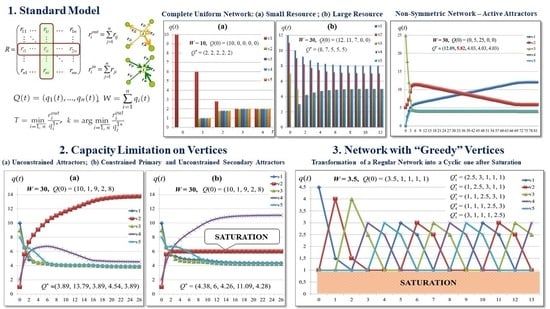
A resource network is a dynamic flow model based on a directed weighted graph. Vertices exchange a homogeneous resource in infinite discrete time. The resource flows through the edges with limited throughputs indicated by their weights. Vertices, in general, can store an unlimited amount of resources. In the network, the conservation law is fulfilled: the total resource amount is constant. In this sense, there are no source and sink vertices in the network; the resource does not come from outside and is not consumed. The network states are described by the vector of the resource distribution over the vertices. The change of states occurs due to the resources reallocation. The resource contained in the edges between two consecutive time steps forms a flow in the network.
For the first time, the resource network was introduced in [1], where a simple special case was considered—a complete uniform network with loops. Since then, the mathematical properties of networks for all graph topologies have been investigated. Some results concerning this paper are presented in [2,3,4,5] (regular networks) and in [6] (Eulerian networks). The classification of resource networks and notions of “regular” and “Eulerian” networks will be given in Section 2.4. The present article summarizes and reinterprets some of the old results obtained for the standard model of a resource network, gives theorems with new proofs, and presents new results—both for the standard model and for two its modifications, as well as for their combination. The first modification is a network with limited vertex capacities introduced in [7]. The second model, a network with “greedy” vertices is defined in [8], where the simple special case, complete uniform networks were investigated.
The study of flows in networks has a long history. In 1962, L. Ford and D. Fulkerson proposed a static flow model and proved their famous “maximum-flow minimum-cut” theorem [9]. Since then, many modifications and extensions of this classical model have appeared; various methods and algorithms are developed to solve different network flow problems [10]. As a rule, these models and methods are devoted to studying homogeneous and heterogeneous flows directed from one or more sources to one or more sinks, possibly with some constraints.
Resource network is a non-linear threshold flow model. Each vertex can send resources to outgoing edges according to one of two rules with threshold switching. The choice of the rule depends on the resource amount at the vertex. If this amount is small (below the threshold value), then the entire resource is distributed in proportion to the throughputs of the edges if it is large (above the threshold value), then the vertex gives to the edges their throughputs and leaves the surplus for itself.
The network with such operation rules inherits the properties of two classes of models. The first one is random walks and diffusion on graphs. This mathematical tool is used to simulate and investigate a wide class of theoretical and applied problems [11,12,13,14,15].
The second class combines integer threshold models. The most studied of them is the model of the combinatorial problem on graphs chip-firing game. This model gave rise to many non-trivial mathematical results [16,17,18,19,20,21]. It is noteworthy that in both classes of models, a special place is occupied by the study of dynamics on regular graphs, in particular, lattices [14,19]. The chip-firing model on different regular directed lattices is proved to be an appropriate mathematical formalism for describing processes of self-organized criticality [22] and, in particular, of Abelian sandpile model [23,24,25]. In this way, the chip-firing game, which is a combinatorial model, and Abelian sandpile model, which is a probabilistic cellular automaton [26,27], are two equivalent forms of one model. In [28], an avalanche model is introduced where the regular lattice of sandpile is generalized to an arbitrary directed graph with multiple arcs. The diffusion game, a parallel variation of chip-firing game, is investigated in [29]. Special mention should be made of networks with different constraints on the flow distribution [30]. Mathematical properties of some of the above and a number of other models are described in a survey [31].
Resource network is both flow and diffusion model. It is completely deterministic, however with small amounts of resource, it is described by a homogeneous Markov chain, which makes it similar to random walks. On the other hand, with large amounts of resource, it becomes similar to a parallel chip-firing game. In this case, it is also deterministic, and its operation is described by a non-homogeneous Markov chain.
The structure of the article is as follows.
In the second section, we will give definitions regarding the basic (standard) model of the resource network and build a classification of networks.
In the third section, we describe the mathematical properties of a resource network.
The fourth section presents the main analytical results for a standard model.
The fifth section is devoted to studying a network with a constraint on the capacity of some selected vertices.
The sixth section describes a resource network with “greedy” vertices and its main features. This is a new model; its research began this year. So far, only complete uniform networks have been described.
The seventh section introduces a combination of two modifications.
Then, we discuss the main findings and research perspectives.
2. Resource Network, the Standard Model
2.1. Basic Definitions
A resource network is a dynamic flow model. It is represented by directed weighted graph with vertices and edges . Edges have the non-negative weights constant in time. The weights specify throughputs of edges.
Matrix is the throughput matrix of a network, . Edge has a throughput equal to .
Definition 1.
Resources are non-negative numbers assigned to vertices and changing in discrete time t. In the standard model, vertices can store an unlimited resource amount.
Definition 2.
A state of a network at time step t is a vector of resource values at each vertex
Definition 3.
A total resource in a network at time t is the value
The network operation fulfills the conservation law: the resource does not flow in from the outside and does not flow out or dissipates:
Definition 4.
Between the two consecutive steps t and , the resource moves along the edges. Such a resource in the edges is called a flow.
is a flow matrix at time t. By definition, .
Definition 5.
The total flow in the network at time step t is the value
Definition 6.
The total throughput of the network is the value
Obviously, .
Remark 1.
Unlike the total resource in the network, the total flow is always limited by its throughput.
In addition, there is an essential difference between states and flows: changes over time if the network is not in an equilibrium state; W is always constant, despite the fact that the values change.
2.2. Rules of Resource Distribution
First, we introduce two characteristics of the network vertices.
Definition 7.
The values
are total in- and out-throughputs of vertex , respectively. A loop’s throughput, if it exists, is included in both sums.
At time step t, the vertex sends to the edge the resource amount equal to
Rule one is applied when a vertex contains more resource than it can send to all adjacent vertices through outgoing edges; in this case, each edge transmits the resource amount equal to its throughput: , and totally, the vertex gives away resource amount
or its total output throughput.
According to rule two, a vertex sends out its entire resource. It distributes the resource to all outgoing edges in proportion to their throughputs.
Remark 2.
The value is the local threshold value of a vertex that switches its functioning rules. This switching occurs without discontinuity: at the value , applying both rules will give the same result.
Unlike the classic chip-firing game, in a resource network, all vertices “fire” in parallel. All non-empty vertices send resource into all outgoing edges at every time step according to rule 1 or 2; adjacent vertices receive the resource through incoming edges.
2.3. Network Operation
First, we introduce the concepts of the output and input total flow.
Definition 8.
For vertex , at time step t, the total output flow is
The total input flow at time step is
We will assume that .
Definition 9.
Vectors and are called the output and input flow vectors, respectively.
The network operates in infinite discrete time. The initial state is determined by the vector of resource distribution over the vertices: .
At time step t, each vertex forms its output flow by one of the rules 1 or 2 (Formulae (1) and (2)). The new state is obtained as follows:
The examples of network operation for the network represented by complete uniform graph are demonstrated in [32].
Definition 10.
The state is called steady if .
Definition 11.
The state is called asymptotically reachable if for some
Definition 12.
The state is called a limit state if it is either steady or asymptotically reachable.
If the state of a network is steady, then the flow is also steady.
Definition 13.
2.4. Classification of Networks by Topology
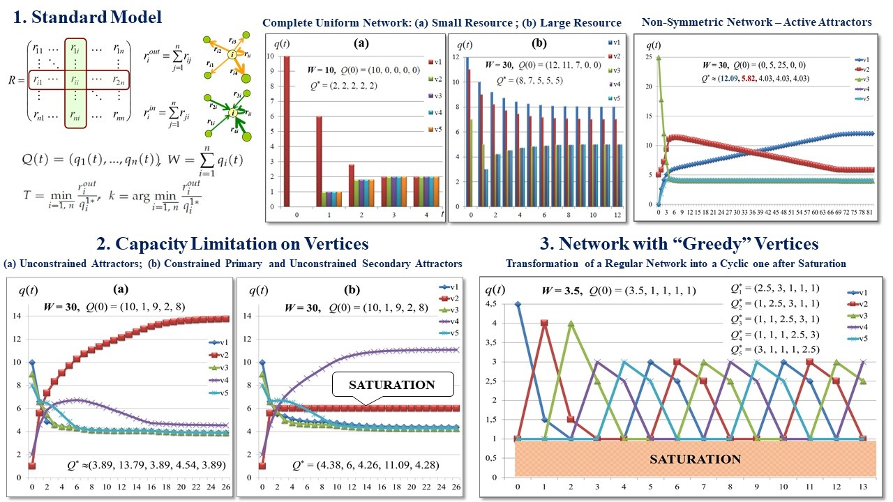
In this classification, the following classes are distinguished (Figure 1).
- Ergodic networks
- Regular networks;
- Cyclic networks;
- Non-ergodic networks
- Absorbing networks;
- Mixed networks.
Definition 14.
A resource network is ergodic if it is represented by a strongly connected graph.
In a random walk on such a graph, any vertex is recurrent. In terms of resource allocation, this means that all vertices both receive and send the resource.
The functioning of an ergodic network at a small resource value (see Section 3.1 for details) is described by an ergodic homogeneous Markov chain [2].
Definition 15.
An ergodic resource network is regular if the greatest common divisor (GCD) of the lengths of all cycles in its graph is equal to one.
Definition 16.
An ergodic resource network is cyclic if GCD of the lengths of all cycles in its graph is more than one.
Definition 17.
A resource network is non-ergodic if its graph is not strongly connected.
Definition 18.
A vertex is called irreversible if there is a path from it to a vertex from which it is unreachable.
Definition 19.
A subnetwork is called transient component if it contains only irreversible vertices.
Definition 20.
A non-ergodic resource network is mixed if it contains transient and ergodic components (Figure 1).
Definition 21.
A mixed resource network is absorbing if all ergodic components are represented by single vertices. Absorbing vertices are an analog of the sink vertices in classical flow networks.
An absorbing network is a special case of a mixed non-ergodic network. On the other hand, a mixed network can be considered an absorbing network if each ergodic component is condensed into one sink vertex.
2.5. Classification of Networks by Total Throughputs of Vertices
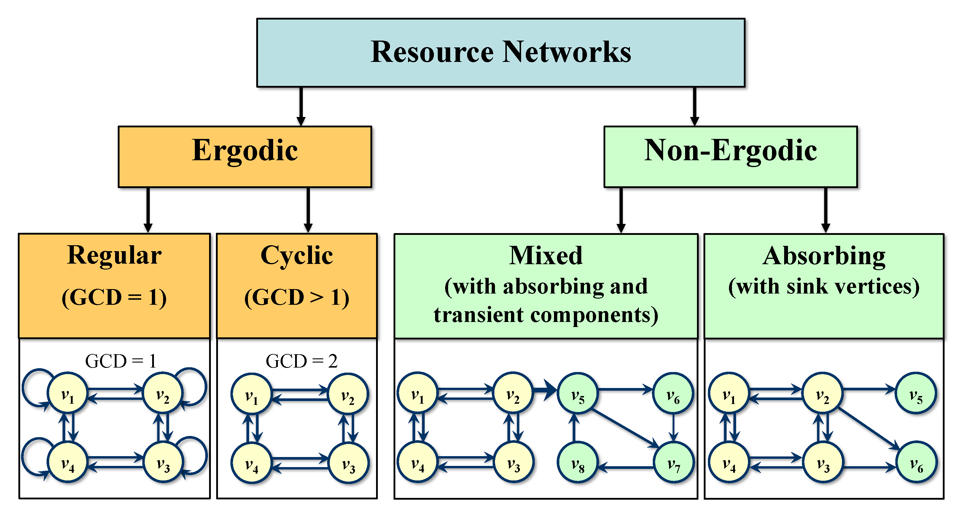
This classification, unlike the previous one, does not have a tree structure. Some classes are not “pure” and may inherit properties from two ancestors (Figure 2).
Definition 22.
A resource network is called uniform if all its edges have the same weights.
We have separated complete uniform networks into a particular class because it is a simple and convenient object for demonstrating various properties of networks.
The nonuniform networks are divided into non-symmetric and Eulerian networks.
Consider the tuple
It characterizes vertices by their total in- and out-throughputs.
If for the vertex , holds , then it can receive more than it can transmit. If , then, accordingly, it can transmit more than it receives. If , this vertex can receive and transmit the same resource amount.
Definition 23.
All the vertices of a network are divided into three classes according to the sign of the value:
- Receiver-vertices, ;
- Source-vertices, ;
- Neutral vertices, .
If at least one receiver-vertex exists in the network, then at least one source also exists, and vice versa.
Definition 24.
A resource network is called non-symmetric if it has at least one receiver-vertex and one source-vertex.
Definition 25.
A resource network is called Eulerian if all its vertices are neutral.
An Eulerian network can be symmetric when the matrix of its graph is symmetric and quasi-symmetric when the matrix is not symmetric, but the equality holds for each vertex.
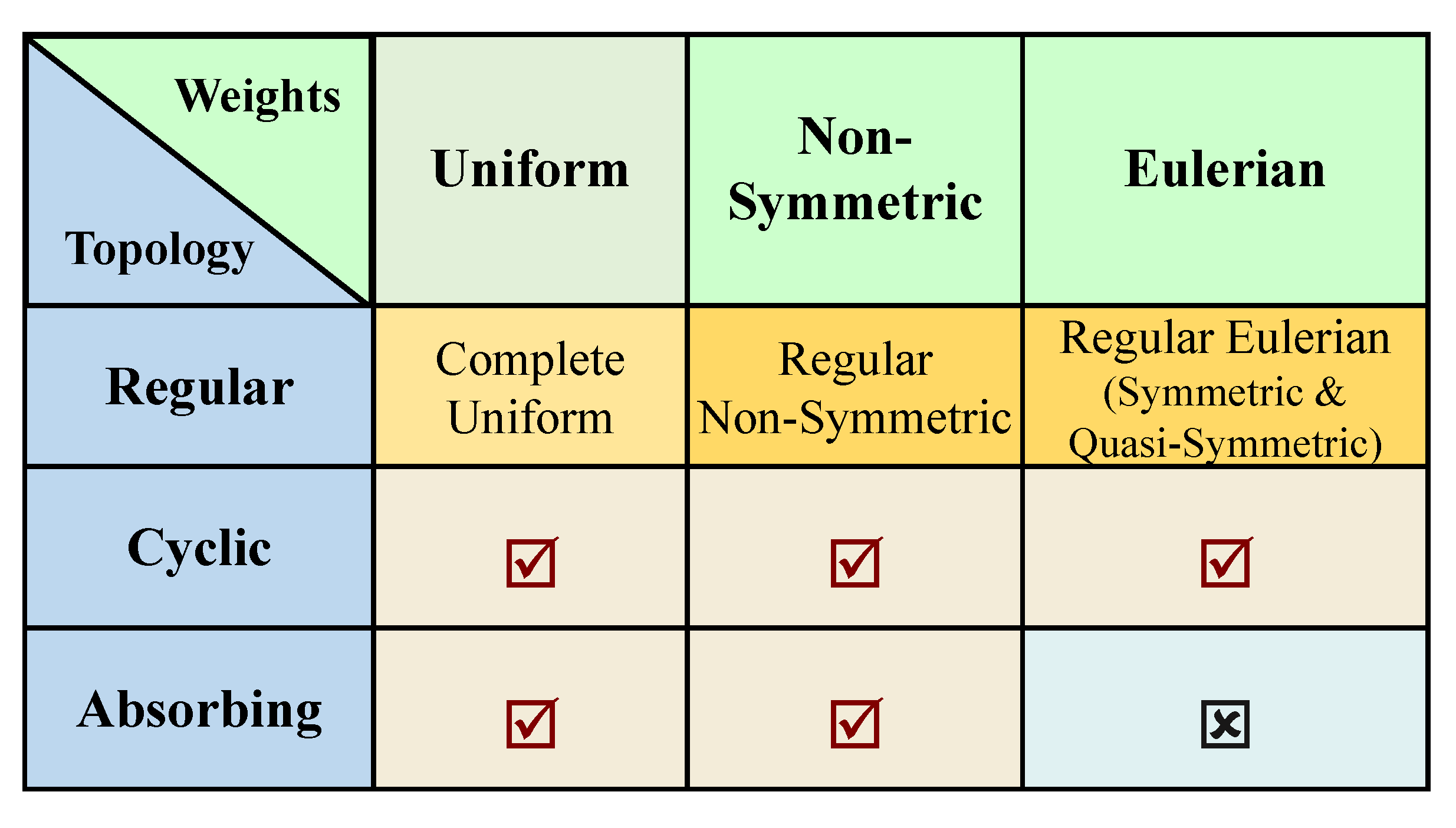
2.6. General Classification of Networks
We introduce a general classification of networks as the Cartesian product of the two introduced classifications (Figure 3).
As mentioned above, uniform networks are an illustrative model example. However, this is not a fully independent class. The results for uniform networks are included in the results for other classes (asymmetric, Eulerian networks) depending on the topology of a uniform network.
This study focuses on the models from the top row of the table in Figure 3. In some cases, they will be considered separately; in other cases, when their properties coincide together.
3. Materials and Methods: The Standard Model
3.1. Regular Resource Networks and Homogeneous Markov Chains
Given a regular network from any throughput-class (the entire top row of the table in Figure 3), consider its operation for the total resource equal to one ().
It was proved that in this case, the resource distribution process is described by a regular homogeneous Markov chain [2].
Denote the vectors of an arbitrary state and of the limit state for as and , respectively.
In this case, the vector is a vector of the initial probability distribution. The transition matrix is obtained from the matrix R as follows:
or , where . is a stochastic matrix.
The change of states is described by the formula
Formula (6) follows directly from the application of rule 2 of the network operation to all vertices. (We assume that the throughputs of the network edges are such that for , all vertices operate according to rule 2).
Therefore, all the results valid for regular homogeneous Markov chains [33] can be transferred to the resource network with .
Proposition 1.
If a regular network is given by matrix R, and matrix is the corresponding stochastic matrix, then
- The limit of degrees of matrix exists:
- The limit state exists and is unique for any initial state.For an arbitrary state the equality holds
- The limit matrix and limit vector are related by the following formula:where .In other words, matrix consists of n identical rows represented by vector .
- Vector is a single left eigenvector of matrices and corresponding to eigenvalue :
Corollary 1.
The limit flow exists and is unique for any initial state: .
If and all the vertices give out their resource according to rule 2, all of the above results will also be correct.
The limit state and flow vectors are unique for any initial state and can be found by the formulae
Lemma 1.
In a regular non-symmetric resource network, for any total resource W and its initial distribution, the resource at source and neutral vertices becomes less than in a finite number of steps (they start functioning according to rule 2).
Proof.
Consider the source and neutral vertices separately.
- Consider an arbitrary source-vertex . Let at its resource be more than its out-throughput: . It operates according to rule 1. At first time step it loses resource amount bounded from below by value . Then it will loose all the surplus in at most steps.
- Let there be neutral vertices in the network.Consider the time step when all the source-vertices switched to rule 2.Consider a neutral vertex adjacent to any source vertex. As the network is regular, such a vertex always exists. Let at its resource be more than its out-throughput: . Then, it loses resource amount bounded from below by value , as the source vertex cannot increase its resource. Then, it will loose all the surplus in at most steps.Consider the next neutral vertex adjacent either to the source vertex or to .Repeating these arguments, we get that in a finite number of steps, all neutral vertices will switch to rule 2.
□
Corollary 2.
In a regular non-symmetric network, if the value W is large, the resource will be accumulated in some of the sink-vertices. Source and neutral vertices can neither attract nor hold a resource in excess of a certain value strictly less than their total out-throughput.
Lemma 2.
In a regular Eulerian resource network, for total resource and any its initial distribution, all the vertices switch to operation according to rule 2. If the switching occurs in a finite number of steps; if resources at some vertices reach the values asymptotically from above.
Proof.
If the proof is similar to the proof of Lemma 1.
Let . As the network is Eulerian, then . Let be the vertex for which inequality holds.
Its output flow is equal to , its input flow does not exceed . The input flow is equal to if and only if for all the rest vertices holds . In this case, , as , and the state is stable.
If and then the value will be reached asymptotically from above. The limit state is .
If and then the value will be reached asymptotically from below. The limit state is .
□
Theorem 1.
In a regular resource network, there exists a unique threshold value of the resource , such that
- if for any initial state , there is a time step , such that if all vertices operate according to rule 2.
- if for any initial state , there will always be at least one vertex operating according to rule 1.
Proof.
It follows from Lemma 1 that in a non-symmetric network all the source- and neutral vertices switch to rule 2 in a finite number of steps .
It follows from Lemma 2 that in an Eulerian network all the vertices switch to rule 2 in a finite number of steps if .
For a non-symmetric network, let the value W be such that all receivers also function according to rule 2.
Consider the functioning of an arbitrary regular network starting from the moment .
It follows from Formula (9) that in this case the limit state exists and .
We will consider the vector as a function of W. Let us increase W until at least one coordinate reach the value .
Denote the limit vector with at least one coordinate satisfying the equality , by .
As the vector is unique, the vector is also unique.
If the resource is increased further, vertex will switch to rule 1.
The resource value at which the equality holds, is the threshold value . It is unique and does not depend on the initial state.
□
Corollary 3.
If , then the limit state and flow vectors are unique for any initial state. They can be found by formula (9).
The following theorem was first formulated in [3] for non-symmetric networks. Here, we generalize it to all regular networks and give a more compact proof.
Theorem 2.
In a regular resource network, the threshold value T is expressed by formula
Proof.
The formula for vector is
Let the vertices with have the indices from 1 to . Then,
or
Then,
This immediately implies Formula (10). □
Definition 26.
The total resource will be called small; the total resource will be called large.
In the following sections, the limit state vector at will play an important role. As the total resource is covered by rule 2, the vector exists and is unique for any regular network. The flow vectors and also exist.
Consider the distinctions in the behavior of regular networks of different classes with a small resource (the top row of the table in Figure 3).
Remark 3.
If , the total steady flow in networks of all these classes is equal to W.
In [32], two examples of uniform complete network operation with small and large resources demonstrate the difference in network dynamics.
3.1.1. Complete Uniform Resource Networks. Small Resource
For complete uniform networks, simpler formulas can be obtained for the limit state and flow vectors, as well as for the threshold value T. This section briefly outlines the results obtained in [1].
The uniform network is defined by only two parameters: the number of vertices n and the throughput of all edges r. The characteristics of a complete uniform network are expressed by the same parameters.
For an arbitrary , the limit vectors are
The limit flow in an arbitrary edge is
If then
The threshold value T is expressed by formula
The limit vectors for are
The resource above the threshold value is not aligned. The limit state depends on the initial state. The network operation with large resources will be considered in Section 3.2.
3.1.2. Eulerian Networks: Small Resource
Complete uniform networks are a special case of Eulerian networks. In Eulerian networks, the equality holds for each vertex . The results obtained for such networks are a generalization of the results obtained for complete uniform networks.
If , then
In the complete uniform network , , whence we obtain its steady state vector (formula (12)).
For an arbitrary the limit vectors are
The threshold value T is expressed by formula
The limit vectors for are
For the complete uniform network, this formula transforms into Formula (13).
3.1.3. Non-Symmetric Networks: Small Resource
For non-symmetric networks, only the most general formulae can be obtained. Vector cannot be expressed only in terms of network parameters. It can be found as the eigenvector of matrices and (Formulae (7) and (8)).
For an arbitrary the limit state vector is
For the threshold value T, a strict inequality holds:
In the limit state, at least one vertex has the resource value equal to its total out-throughput
and at least one vertex has the resource value strictly less than its total out-throughput
Let there be l vertices satisfying the condition (18) in a network, . Introduce such numbering that these vertices have the first numbers. Then, the limit vectors for are
Comparing Formula (19) with Formulae (13) and (16), we find that for complete uniform and Eulerian networks, the equality holds. For non-symmetric networks, the strict inequality is required.
As the threshold value is equal to the sum of the coordinates of vector , the nature of inequality (17) becomes clear.
3.2. Regular Networks. Large resource
3.2.1. Non-Symmetric Networks
In this section, for introducing a number of properties, we turn first to non-symmetric networks.
When the resource in the network is above the threshold, some vertices start accumulating surpluses. It is natural to assume that these are the receiver-vertices (see Definition 23).
Examples with different networks functioning are considered in [32] (Examples 3–5). Example 5 demonstrates that not all receivers can accumulate a resource surplus. Moreover, based only on the network topology and characteristics of the vertices , it is not always possible to determine which of the receivers will attract the resource.
Let us introduce the concept of an attractor vertex.
Definition 27.
A vertex capable of accumulating a surplus of resource is called an attractor vertex.
Attractors can be receiver-vertices and some neutral vertices. Results for neutral vertices will be presented in Section 3.2.2.
Receivers are active attractors. They can attract the resource from other vertices.
Neutral vertices can only partially keep the surplus if they already have it. Such attractors will be called passive.
3.2.2. Complete Uniform and Eulerian Networks: Large Resource
For the complete uniform network with parameters n and r, the threshold value is , and the limit vector is defined by Formula (13):
Let . Consider an arbitrary initial state. There exists at least one vertex in a network for which holds
This vertex has a surplus equal . Let us denote this surplus as . At least at time step this vertex will operate according to rule 1.
Arrange the vertices in descending order of their resource.
Let there be l vertices in a network satisfying condition (20). Then, the vector of initial distribution has the form
where are deficits of resources to value .
The total surplus in a network at is denoted as and the total deficit as :
If then and .
Experiments show that in a complete uniform network with the initial distribution given by (21) the limit state exists. It has a form
where . The Example 6 in [32] shows both these cases: and .
Proposition 2.
In the complete uniform network with parameters , for given if
then and
where
otherwise.
This statement is demonstrated in Example 6 [32].
For an arbitrary Eulerian network, all the results obtained for complete uniform networks are transferred almost unchanged as any vertex of the Eulerian network is also a passive attractor. However, finding the limit state with a large resource is much more complicated (Section 4.3).
4. Results: Standard Model
In this section, we present the main results for regular resource networks.
4.1. Non-Symmetric Networks
In Definition 27, we introduced a notion of an attractor vertex. In general, this is a vertex that can have resource surpluses in the limit state at .
Except for some special cases, in asymmetric networks, the attractors are always receiver-vertices. Experiments show that not every receiver-vertex can be an attractor. Moreover, the Example 4 in [32] demonstrates that in a number of cases, it is impossible to recognize an attractor only by the topology of the graph and the total capacities of the vertices. An attractiveness criterion is formulated and proved in [4]. Here, we give a much shorter proof. This criterion is universal. It is suitable for all classes of resource networks, not just regular ones.
Theorem 3.
The vertex of resource network is an attractor if it satisfies the equality
Proof.
The minimum of this ratio is achieved on the attractor vertices. Therefore, vertex is an attractor if and only if Formula (22) is true.
□
The following theorems determine the limit states and flows in a regular asymmetric network for any total resource and its initial distribution. They summarize the above results.
Theorem 4.
The limit state in an asymmetric regular network with l attractor vertices exists for any total resource W.
- 1
- If then vector is unique and defined by the formulawhere is the limit stochastic vector of corresponding homogeneous regular Markov chain with stochastic matrixAll components of are positive.
- 2
- If then vector is unique and has the formwhere vertices with first indexes are attractor vertices; the rest vertices satisfy the strict inequality
- 3
- If , then vector has the formwhere , are resource surpluses distributed among attractors:The values of depend on the initial distribution.
Theorem 5.
The limit flow in an asymmetric regular network with l attractor vertices exists and is unique for any total resource W. Vectors and are defined as follows.
- 1
- If thenAll components of matrix are positive.
- 2
- If thenwhere vertices with first indexes are attractor vertices; the rest vertices satisfy the strict inequality
Remark 4.
For any arbitrarily large resource , the total flow is limited by the value T.
As follows from the theorems, the resource is accumulated only by the attractor vertices. The rest of the vertices at have the same small amount of resources, no matter how large W is.
To investigate a more even distribution of the resource, we created a model with constraints on attractors. It will be described in Section 5.
4.2. Complete Uniform Networks
In Eulerian networks in general, and in complete uniform networks in particular, each vertex is an attractor. This feature determines their behavior with a large resource. All vertices are passive attractors. They can hold a resource at certain initial states, but they cannot accumulate it.
We remind that for a complete uniform network, the threshold value is .
First, describe the results for complete uniform networks. Uniform complete networks were introduced and investigated in [1]. However, in that work, the apparatus of converging series was used, which was reflected not only in the proofs, but also in the formulation of the statements. In the present article, the results obtained are structured and simplified. All theorem proofs are new.
Theorem 6.
The limit state in a complete uniform network exists for any total resource W. For , it is unique.
- 1
- If then
- 2
- If then
- 3
- If , then vector depends on the initial stateand has the formwhere , are resource surpluses:The values of depend on the initial distribution.
- Ifthen ant the limit state has the form (Proposition 2):
- Ifthen is the highest index for which the inequality holdsand the limit state vector iswhere
Proof.
The validity of items 1 and 2 follows directly from the results obtained for regular homogeneous Markov chains [33].
Consider an arbitrary initial state of the network for where the vertices are ordered in descending order of the resource (Formula (23)). As the network is complete and uniform, all vertices have the same input flows. The output flow of the first l vertices is equal to . The remaining vertices give all their resources equally to all other vertices of the network. Then, all vertices during the network operation must give the resource equally. The resource at each vertex must decrease by .
- If then the limit state is described by the Formula (25).
- If then perform a number of steps.
- Reduce the surplus in each of the first l vertices by the value .
- Distribute the resource equally between the vertices .
- Take the resulting vectoras a new initial state .
- Calculate the new value of the total deficit:
- Evaluate the new value .
- –
- If then and the limit state is described by the Formula (26).
- –
- If then all steps must be repeated.
The limit state will be found in at most iterations and is expressed by the formula (25) or (26) depending on the condition (24).
□
The limit flow is defined by the following theorem.
Theorem 7.
The limit flow in a complete uniform network exists and unique for any total resource W.
- 1
- If then
- 2
- If then
4.3. Eulerian Networks
The threshold value for Eulerian networks is .
For , let the vector of initial distribution be where
The following theorem was proved in [6].
Theorem 8.
The limit state in an Eulerian network exists for any total resource W. For , it is unique.
- 1
- If then
- 2
- If then
- 3
- If , then vector depends on the initial state and has the formwhere are resource surpluses:The values of depend on the initial distribution.
Remark 5.
For , the relationship between the initial and limit states in Eulerian networks is much more complicated than this relationship in complete uniform networks. It is not enough to arrange the vertices in descending order of surpluses to find out which of them will not be able to hold the resource. In formula (27), some of the first l vertices may have zero surpluses.
This remark is illustrated by Example 7 in [32].
4.3.1. Initial State Analysis
First, consider symmetric networks. The behavior of quasi-symmetric networks is more complicated. If a network is symmetric, every vertex has paired in- and out- edges with the same weights, so the flows between these vertices are also symmetric. The flow sent by vertex along the output edge into vertex , returns along the coupled input edge . Therefore, the flow within the subnetwork of the first l vertices is constant. In quasi-symmetric network this symmetry is violated.
Let and the initial state has the form
The total deficit is denoted as , the total surplus as . For , , and .
The vectors of deficit and surplus at time t are
Then
Formulate the problem as follows.
Let the vector of initial deficits is known. Find a vector of initial surpluses
at which none of the first l vertices will switch to rule 2 during the network operation. This is a necessary and sufficient condition for (item 3 of Theorem 8, Formula (27)).
When this vector is found, for any initial state with , for each of the first l vertices it will be possible to determine its surplus in the limit state: . Generally, if , finding the vector is equal to finding the limit state vector, as
where
Comparing vectors and
we get the formula
where
Here, is the identity matrix of size ; is the zero matrix of size , and are corresponding blocks of matrix :
It follows directly from (29) that
where The formula for is obtained in [6].
where is the identity matrix of size .
Split vector into two components: of length l, and of length .
Proposition 3.
Let and . Then, the first l coordinates of vector (28) are found as follows:
Proof.
- If , the deficits in the corresponding vertices are , and the proof follows from Formula (32).
□
In [6], an algorithm for finding the limit state is proposed for the case . It is based on the same principles as Theorem 6, formulated for complete uniform networks, but in the case of arbitrary symmetric networks, the formulas are more cumbersome.
4.3.2. Operation Analysis
Write out the formulas for changing the network states with a large total resource. Again, assume that the first l vertices at each time step operate according to rule 1.
By definition,
Then
It is easy to see that where L is the normalized Laplacian matrix.
Generally,
The sequence of vectors converges to . The sum does not converge as , as is not equal to the zero-matrix (Formula (31)). However, tends to , which, in turn, is the unique eigenvector of matrix . Therefore, tends to the zero vector. Passing to the limit, obtain
As t is an arbitrary time step, then
where
Then,
On the other hand, . Then,
If for a given network, and given vector then
The first l coordinates of this vector are defined by Formula (33), the remaining are equal to zero.
The flow behavior in Eulerian networks is much simpler to describe. The flow in an arbitrary Eulerian network (both symmetric and quasi-symmetric) with depends only on its throughputs. Each edge is filled completely.
Theorem 9.
In an Eulerian network, the limit flow exists and is unique for any total resource W.
- 1
- If , then
- 2
- If , then
Proof.
The proof follows directly from the properties of homogeneous Markov chains, since unlike network states, flows are always described by homogeneous chains. □
5. Resource Network with Limited Capacity of Attractor Vertices
In this section, we consider only non-symmetric regular networks, as in Eulerian networks, each vertex is a potential attractor, and there is no point in limiting such vertices. In non-symmetric networks, for any arbitrarily large resource, attractors accumulate all the surplus. Capacity limitations are introduced for a more even distribution of the resource.
A vertex is an attractor of an asymmetric network if it satisfies criterion (22). In this modification of the standard model, such vertices will be called primary attractors. For such vertices, we impose a limitation on the capacity of the following form
This limitation applies only if ; otherwise, for a given initial state, the capacity of the vertex will remain unbounded.
The form of constraint (34) is due to the fact that for attractor , the equality holds. And is some constant value limiting resource surplus .
The following two propositions are proved in [29].
Proposition 4.
In a regular non-symmetric network with restrictions, there is a second threshold value of the total resource , :
- if , the network operates as a network without capacity limitations;
- if , the dynamics of the network changes,
where l is the number of attractors.
Proposition 5.
For the values of total resource W, there are four intervals with different network functioning.
- For , from some moment the network operation is described by a homogeneous Markov chain. The limit state and flow vectors exist, are unique and coincide. The total limit flow is equal to W and increases with the growth of W.
- For , the limit state and flow exist. The limit flow is unique, the limit state is unique for ; for , the limit state is unique at all vertices, except attractors. The resource in attractors is not less than their output throughputs. The surpluses in attractors depend on the initial distribution of the resource, but the sum of these surpluses does not depend on the initial state and is equal to . The total limit flow is equal to T and does not change with increasing W.
- For , all attractors reach a capacity limitation. An excess resource begins to accumulate in the remaining vertices, but none of them is still able to exceed the value , that is, switch to rule 1 operation. The total limit flow is equal to and increases with the growth of W.
- For , the new vertices are saturated to the total output and the flow is stabilized at the value . For any arbitrarily large value of W, the total limit flow is equal to .
If the limitations of attractors are equal to zero , the second interval disappears and three remain: .
Definition 28.
The vertices that saturate to the total output throughput when are called secondary attractors.
Example 8 in [32] illustrates the concept of a secondary attractor. It demonstrates the functioning of an asymmetric network with a total resource W belonging to the last interval .
The first two intervals of the total resource in Proposition 5 specify the conditions under which restrictions on attractors do not apply, and the operation of the network is standard.
Consider the two remaining intervals. Without loss of generality, we assume that .
5.1. Network Operation with Resource
In this interval, such a moment exists when all attractors are saturated. Then they cannot receive the entire input flow and start to return its part back; and this part is redistributed between the non-attractive vertices. For all the operation of a network can be described by formula
where are excess surpluses of the input flow in saturated attractors, which are redistributed between other vertices. They are expressed by formula
Note that in formula (35), for all flows holds . This means that these are flows from non-attractive vertices, and according to rule 2, they are equal to the fractions of
Then, expression (35) can be rewritten in terms of .
In the matrix form, it is written as
where is the stochastic matrix of a standard network (Formula (5)). To define matrix , we introduce additional notation.
As in the previous section, represent the matrix in block form (30).
Block has dimension and corresponds to attractor vertices.
Then matrix can be expressed in terms of blocks of matrix and values,
where and are the identity matrices of size and accordingly; is the zero matrix of size .
Proposition 6.
is a stochastic matrix.
Proof.
Consider the two lower blocks of matrix .
The diagonal elements of matrix are positive. The values in this matrix are the sums of the elements of the corresponding row of matrix (37). Then, the total sum of elements of each row is equal to one. □
Proposition 7.
is an invertible matrix. The inverse matrix is expressed by formula
where
Proof.
It is easy to verify that for the matrix given by Formula (38), the equality holds
□
Due to this proposition, Equation (36) can be rewritten to find .
Proposition 8.
where is a column vector of ones.
As matrix has negative elements, it is pseudo-stochastic.
Remark 6.
For different networks, matrix can be stochastic or pseudo-stochastic. The work in [34] introduces reversible network transformations that convert a pseudo-stochastic matrix into a stochastic one. Without loss of generality, we will assume that the matrix is stochastic. Then, the equality (39) describing the operation of a network defines a heterogeneous Markov chain [35].
The network operation is described as follows:
Definition 29.
A heterogeneous Markov chain with stochastic matrices is called strongly ergodic if
where 1 is a column vector of n units, π is a certain probability vector.
Proposition 9.
The heterogeneous Markov chain with stochastic matrices is strongly ergodic.
Proof.
First, prove that exists.
For the first l components of vector tend to values by definition of a network with attractor limitations.
It means that two left blocks of have limits; and then the sequences converge and two right blocks also have limits.
The sequence converges. Therefore, the sequence converges too. Let .
Consider matrix . This is a regular stochastic matrix and then it defines a homogeneous Markov chain. Thus,
and therefore
□
Theorem 10.
In a regular non-symmetric network with a limited capacity of attractors for , the limit state exists, is unique, and is an eigenvector of matrix
The proof the proof follows directly from Proposition 9.
5.2. Network Operation with Resource
All the statements in this section are proved in [34].
Theorem 11.
The second threshold value , for which at least one non-attractive vertex has the limit resource , is unique.
The limit state vector at is denoted by .
Matrices depend not only on time but also on the total amount of resource W in the network.
The limit matrix at is denoted by .
Matrix is expressed by formula
The limit state vector is the left eigenvector of matrix with eigenvalue :
Proposition 10.
The limit of powers as exists and is equal to the limit matrix of a homogeneous Markov chain with limit probability distribution :
where 1 is a column vector of n units.
Corollary 4.
Each network with limitations can be uniquely associated with a regular homogeneous Markov chain with matrix defining a new network without constraints (a standard model) with the following parameters:
- ;
- the threshold value ;
- the limit state vector at is ;
- the limit of powers of the stochastic matrix is
Proposition 11.
A non-attractive vertex of a regular asymmetric network is a secondary attractor of this network with limitations if and only if, for , it satisfies the condition
Matrix is stochastic (see Remark 6). Any stochastic matrix defines a family of networks, which corresponds to a family of throughput matrices, the corresponding rows of which are proportional. Let be the matrix of the network whose threshold value T coincides with of the original network. Moreover, for all primary and secondary attractors, the equality will hold, i.e., both the primary and secondary attractors of the original network are the primary attractors of the induced network. Such a network is given by the formula
Thus, knowing the limit vector of resource distribution at in a network without limitations given by matrix R, it is possible to construct a homogeneous Markov chain and the induced matrix such that at , their limit states coincide.
Now, we can formulate the criterion of secondary attractiveness.
Theorem 12
(Secondary Attractiveness Criterion). A non-attractive vertex of a regular asymmetric network without constraints with matrix R is a secondary attractor if and only if in induced network it satisfies
where are coordinates of limit vector of induced network with .
Theorem 13
(Threshold theorem). The second threshold value of the network with constraints is determined by the formula
The Limit State Theorem summarizes the results of this section.
Theorem 14
(Limit State Theorem). In a regular non-symmetric network with constraints on attractors p, the limit state exists for any value of the total resource W. There are two threshold values T and , such that:
- For , the limit state is unique and is found by the formula ;
- For , the limit state is unique for ; for , the limit state is unique at all vertices, except for attractors:where are components of limit vector at ;
- For , the limit state is unique. It consists of the sum of two vectors . Here ; is the limit state of an induced network with matrixIf , then this equality transforms into formula (40) and the limit state isthe vertices are the secondary attractors.
- For , the limit state is unique up to surpluses in the secondary attractors. It is found by the formulais the left eigenvector of matrix corresponding to the maximum eigenvalue ; are surpluses of resource in excess of the value, distributed among secondary attractors.
6. Resource Network with Greedy Vertices
Consider a resource network with loops and define its functioning as follows. At time step t vertex sends to the loop the resource value equal to
If the remaining resource is distributed among other vertices according to the rules of the standard resource network.
Thus, the nodes of the network are “greedy”; they allocate the available resource first of all to themselves.
Definition 30.
We will say that the network stopped at time step if .
Remark 7.
Note that in the first two described models, the network did not stop at any resource value. The stop is a new state that has appeared in a network with greedy vertices.
Proposition 12.
The network stopped at time step if and only if .
The proof of this proposition follows from the rules of the network operation.
Definition 31.
Given time step t, vertex is called unsaturated if , saturated if , and oversaturated if .
Definition 32.
The resource at the vertex in excess of the loop throughput is called free and denoted as
Proposition 13.
A vertex saturated at time t will also remain saturated at time .
6.1. Two Threshold Values
There is one threshold value T of total resource W in a standard resource network. This threshold divides the resource into small values, when all vertices give away their entire resource at each time step, and large values, when resource surpluses accumulate in one or several vertices.
In resource networks with greedy vertices, there are two threshold values and , which separate zones of different network behavior. If the network stops—in a finite number of time steps, or asymptotically, depending on the initial state.
Definition 33.
The total resource value at which the network stops operating is called insufficient; otherwise, it is called sufficient.
The threshold value separating insufficient and sufficient resources is denoted by . The threshold value at which at least one vertex switches from rule 2 to rule 1 is denoted by .
Proposition 14.
The first threshold value of the resource of a regular network with greedy vertices is unique for any initial state and is found by formula
Theorem 15.
If the total resource , all the vertices of a regular network are saturated in a finite number of time steps.
Proof.
Consider an arbitrary vertex with the resource value . As and the network is regular, its input flow . Its output flow is equal to zero. Then, at each time step the resource of the unsaturated vertex increases by a positive value bounded from below, as the total flow is strictly positive and does not tend to zero. If and all the vertices operate according rule 2 then
If the flow is bounded from below at least by the sum of all out-throughputs of vertices operating according to rule 1.
Therefore, is bounded from below at every step t by a strictly positive constant . The number of the time steps for its saturation is not greater than . □
The following theorem is important since it allows to reduce the study of networks with greedy vertices to the standard model, passing to a new initial state, when .
Theorem 16.
For , a regular resource network with greedy vertices from moment operates equivalently to the corresponding standard resource network without loops, in which the resource at each vertex is reduced by the loop throughput .
Theorem 17.
The threshold value of a network with greedy vertices coincides with the threshold value T of a corresponding standard model.
The proofs of these two theorems follow from the definition of the resource allocation rules in a network with greedy vertices.
These theorems show that only two cases are of interest for networks with greedy vertices.
The first case is . The resource is absorbed by the loops during the network operation. Such a network can be considered as an absorbing network with sink vertices corresponding to unsaturated greedy vertices. The main difference is that a greedy vertex can saturate and start giving up the resource, while this is impossible for a sink vertex.
The second case is a violation of the regularity of the network when removing loops. Below we consider both cases.
6.2. Insufficient Resource
Proposition 15.
The network stopped at time step if and only if there is no such cycle in the network that and for every t, at least one inequality is strict.
Proof.
1. Consider the cycle where all the vertices are saturated and, at every time step, at least one of them is oversaturated. The vertex that has become saturated remains saturated in the future. The part of the free resources of oversaturated vertices will be dispersed to other unsaturated vertices, but the other part will still stay inside the cycle. Then, the network will not stop.
2. If the network stopped, then all free resource was absorbed by the loops, which means that there is no saturated cycle in the network. □
Note that the unsaturated vertex only accepts the resource, but does not give it away. This means that if we eliminate all of its outgoing edges, the network operating will not change. Thus, unsaturated vertices in the regular network correspond to sinks in the absorbing network.
Depending on the total resource and its initial allocation, some unsaturated vertices may become saturated over time. However, some of them will remain unsaturated, since .
Let be the time step starting from which the set of unsaturated vertices has stabilized and let these vertices have indices . Then, matrix R can be represented as follows:
Here, the weights of all outgoing edges of unsaturated vertices are equal to zero. D is a diagonal matrix with weights of loops, and are the unchanged blocks of matrix R.
The corresponding stochastic matrix has a form
Its powers are
The two results follow directly from Theorem 1.11.1 in [33]: (1) matrices tend to zero matrix, and (2) the series converges to matrix . Therefore, the limit of powers exists and is expressed by the formula
Theorem 18.
Matrix remains unchanged for any changes in the diagonal elements of matrix R.
Proof.
Consider the new matrix where is the diagonal matrix with arbitrary values .
The blocks of a new stochastic matrix will have a form
This imposes a constraint on : . To fulfill this condition at the first l vertices, we assume that .
Substitute these values into the expression for the matrix . Let
Therefore,
All the diagonal elements of matrix are nonzero then it is invertible. Therefore,
Thus, we have that
and . □
Theorem 19.
Let the set of unsaturated vertices not change from time step and these vertices have indices from 1 to l. Then, the limit state of the network is found by the formula
Proof.
If for all vertices operate according to rule 2, the proof is obvious, since the network is described by a homogeneous Markov chain.
Let some of vertices operate according to rule 1. Since the network is absorbing, and these vertices are in the transient component, they will lose surplus in a finite number of time steps . During the time interval , the network will be described by an inhomogeneous Markov chain with stochastic matrices corresponding to the matrices , differing from each other by the weights of some loops. The elements of stochastic matrices are
The limit vector is described by the following expression:
Prove that for arbitrary matrix , the equality holds , where has the form (41).
As matrices differ only in diagonal elements, the two lower blocks of the matrix can be represented as , , where and are defined by formula (42). Consider the product
Transform the bottom left block
Note that
thus
We obtain that , and
□
6.3. Greedy Vertices and Cyclic Networks
Theorem 16 has an important corollary. In Section 2.4, a notion of a cyclic resource network was introduced (Definition 16). In a cyclic network, the greatest common divisor of the lengths of all cycles is greater than one. Note that even a single loop turns a cyclic network into a regular one. The reverse process, i.e., the elimination of all loops, can turn the regular network into a cyclic one.
Definition 34.
Let the GCD of all cycles of a network without loops be . Such a network with greedy vertices is called d-cyclic.
Theorem 20.
If, after removing the loops in the standard model, the regular network turns into a d-cyclic one, then in a network with greedy vertices for there is a limit cycle with d limit vectors .
This theorem is illustrated by Example 9 in [32]. Its proof follows from the definition of a network with greedy vertices.
Consider the network operation with the resource value satisfying inequality , i.e., with sufficient small resource. The results listed below are obtained for cyclic networks of the standard model in [36].
Let is the throughput matrix of a d-cyclic network with greedy vertices where all diagonal elements are replaced with zeros.
Let be the stochastic matrix corresponding to . The sequence of its powers: . It consists of d convergent subsequences:
(1)
(2)
...
(d)
Matrices of each subsequence have zero elements in the same places.
All limits of these subsequences are expressed in terms of one limit matrix
Then, these limits are
A saturated d-cyclic resource network has a limit cycle of length d:
Here, is a vector of state at any time step , when all the vertices have already saturated and operate according to rule 2.
Each vector cyclically passes to the next one:
Vectors are eigenvectors of matrix corresponding to the eigenvalue of multiplicity d.
If these vectors coincide, then the network has an equilibrium state. The equilibrium vector is vector , where is any row of Cesaro limit matrix A:
Vector is the unique positive eigenvector of the matrix . It can be calculated as
for any .
For a large resource , the cyclic nature of the network ceases to matter. For such a network, all the results obtained for regular networks in the standard model are true. The limit state and flow exist. The limit flow is unique. The limit state is unique up to the surplus of resources in the attractors. The attractiveness criterion remains unchanged.
7. Resource Networks with the Limited Capacity and Greedy Vertices
Consider combining two modifications of the standard model. The models are completely independent. Features of a network with limitations on attractor capacities appear at a large resource, features of a network with greedy vertices appear at an insufficient resource. However, both of these models allow vertices to accumulate resource at different intervals. Primary and secondary attractors can attract a resource due to the structure of their connections; greedy vertices can only use the capacity of their loops.
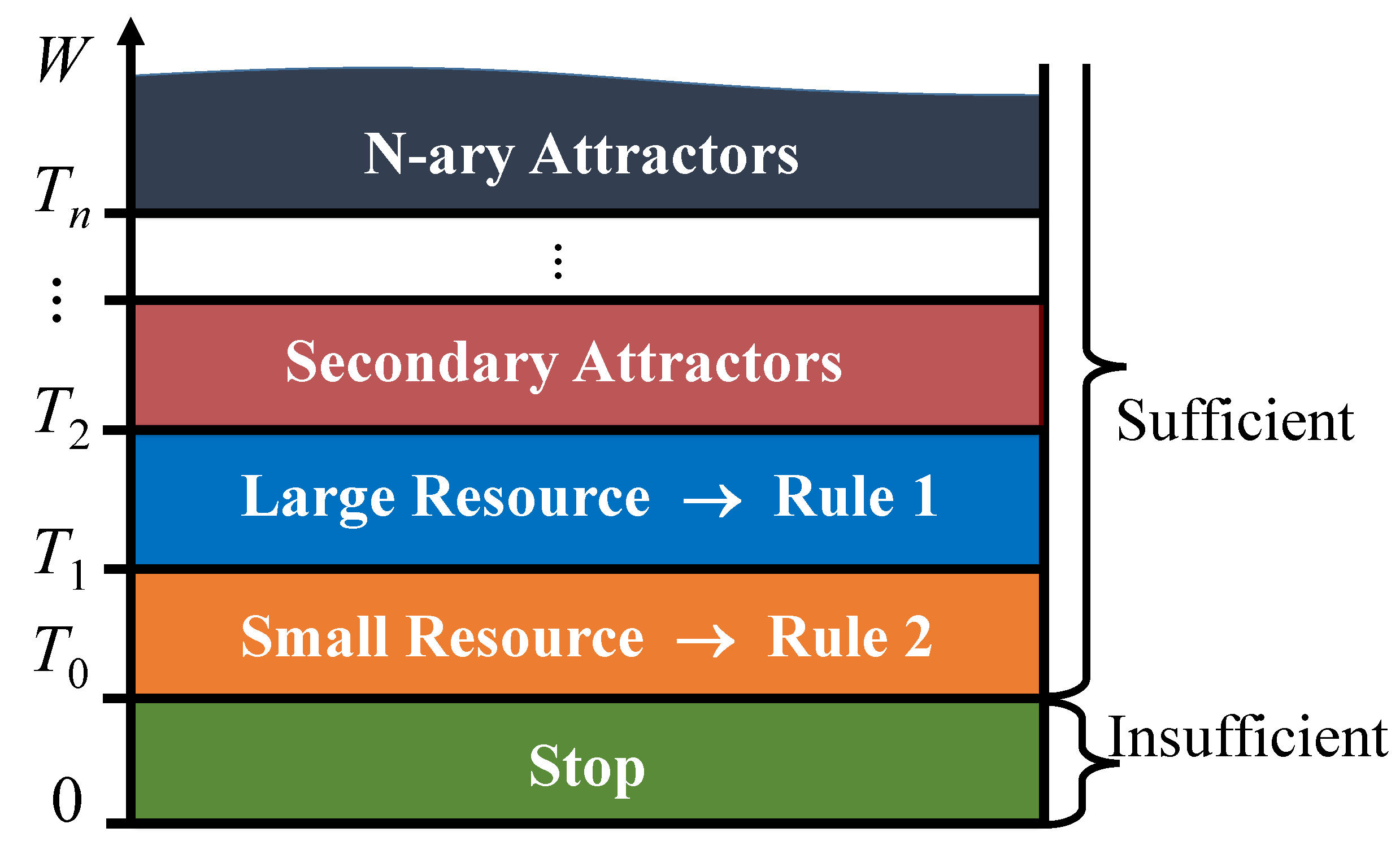
The combination of the two models will allow the vertices to have both features. The new model will have three thresholds. This process can be continued. By limiting the secondary attractors, we obtain attractors of rank 3, etc. (Figure 4).
8. Discussion
Resource network is a graph dynamic model with threshold switching of functioning rules. Transient processes and limit states depend on the topology of the graph and the weights of its edges, as well as on the total network resource, and, in some cases, its initial distribution. Each vertex operates according to one of two rules of functioning, depending on the available resource. The local threshold value of vertex is equal to its total out-throughput . Despite many local thresholds, it has been proven that there is only one global threshold T in the network. If the total resource has exceeded this threshold, the network ceases to be described by a homogeneous Markov chain. Some vertices begin to accumulate surplus resources. They are called attractor vertices. If the graph weights are given by rational random variables, there is a single attractor in the network with a probability equal to one. However, for any stochastic matrix, it is possible to create a network with an arbitrary number of attractors. If every vertex in the graph is an attractor, the network generated by this graph belongs to the class of quasi-symmetric networks. A special case of quasi-symmetric networks is a class of complete homogeneous networks, a convenient tool for illustrating the various properties of resource networks.
A criterion of vertex attractiveness is formulated and proved. Attractors can be active and passive. Active attractors are receiver vertices in an asymmetric network. Passive attractors are neutral vertices in symmetric and quasi-symmetric networks. Active attractors attract resources from other vertices. Passive attractors are only able to keep it. Thus, in a passive attractor, the property of “attraction” is manifested only in potency—it depends on the initial resource allocation. An active attractor accumulates surpluses regardless of the initial state.
Two different modifications of the standard resource network model are proposed. The first describes a model with constraints on attractor vertices. This model allows redistributing surplus resources more evenly. Other vertices appear in the network, accumulating surpluses. They are called secondary attractors. Vertices that are neither primary nor secondary attractors also slightly increase their resources in the limit state. A non-homogeneous Markov chain describing the operation of a network with limitations on attractors is constructed. Its strong ergodicity is proved. Based on the obtained non-homogeneous Markov chain, a homogeneous chain and a matrix of weights are constructed, describing the functioning of a new resource network, in which the primary attractors are the primary and secondary attractors of the original network. The criterion of secondary attractiveness is formulated and proved. It is proved that in a network with constraints, there is a second threshold value, and a formula for its value is found. The behavior of networks is investigated in each range of resource values bounded by the thresholds.
By limiting the secondary attractors, the attractors of the rank three can be found. Continuing this operation, you can rank all the vertices of the network by the rank of attraction. In this case, the attractiveness rank can serve as a new measure of the vertex centrality in a graph.
In the second modification of the model, the network with greedy vertices, the vertices first take the resource for themselves and only then begin to give the rest to other vertices. The resource reserve of a vertex is equal to the throughput of its loop. A new state appears in this network, a network stop. In the two previous models, this state was impossible. Two cases of interest are considered: the case of insufficient resource and the loss of regularity with a large resource.
Of particular interest is the fact that these networks also have a second threshold value. However, in networks with limitations, the additional threshold value is greater than the first, and in networks with greedy vertices, it is less than first.
For networks with greedy vertices, only the first results are obtained. Complete homogeneous networks are investigated [8]. The present paper considers the general case–regular networks with an arbitrary topology. New results are obtained for networks with insufficient resource. A formula for the limit state is obtained, theorems are proved on the independence of the resource allocation from the loops’ throughputs. In terms of matrices, this means that the limit of the powers of stochastic matrices does not depend on the diagonal elements of the original matrix.
Further research will include a description of the remained classes of networks. It is planned to develop resource networks on graphs with constraints imposed on some selected arcs. A separate large area is the development of applications using resource networks in various subject areas, in particular, in telecommunication technologies.
The following abbreviations are used in this manuscript:
Funding
This research was funded by the Russian Foundation for Basic Research (projects Nos. 20-07-00190-a, 19-07-00525-a, 18-29-22042-mk).
Institutional Review Board Statement
Not applicable.
Informed Consent Statement
Not applicable.
Data Availability Statement
Not applicable.
Acknowledgments
The author thanks Oleg Kuznetsov for inventing the resource network and many inspiring discussions, and Nadezhda Chaplinskaya for her collaboration in the study of networks with greedy vertices. I am very grateful to the reviewers for their constructive and inspiring comments.
Conflicts of Interest
The authors declare no conflict of interest.
References
- Kuznetsov, O.P. Uniform Resource Networks. I. Complete Graphs. Autom. Remote Control 2009, 70, 1767–1775. [Google Scholar] [CrossRef]
- Zhilyakova, L.Y. Asymmetrical Resource Networks. I. Stabilization Processes for Low Resources. Autom. Remote Control 2011, 72, 798–807. [Google Scholar] [CrossRef]
- Zhilyakova, L.Y. Asymmetric resource networks. II. Flows for large resources and their stabilization. Autom. Remote Control 2012, 73, 1016–1028. [Google Scholar] [CrossRef]
- Zhilyakova, L.Y. Asymmetric resource networks. III. A study of limit states. Autom. Remote Control 2012, 73, 1165–1172. [Google Scholar] [CrossRef]
- Zhilyakova, L. Resource Allocation among Attractor Vertices in Asymmetric Regular Resource Networks. Autom. Remote Control 2019, 80, 1519–1540. [Google Scholar] [CrossRef]
- Zhilyakova, L.Y. A study of Euler resource networks. Autom. Remote Control 2014, 75, 2248–2261. [Google Scholar] [CrossRef]
- Zhilyakova, L.Y. Resource Network with Limited Capacity of Attractor Vertices. Autom. Remote Control 2019, 80, 543–555. [Google Scholar] [CrossRef]
- Zhilyakova, L.; Chaplinskaya, N. Research of complete homogeneous “greedy-vertices” resource networks. UBS 2021, 89. (In Russian) [Google Scholar] [CrossRef]
- Ford, L.R., Jr.; Fulkerson, D.R. Flows in Networks; Princeton Univ. Press: Princeton, NJ, USA, 1962. [Google Scholar]
- Ahuja, R.K.; Magnati, T.L.; Orlin, J.B. Network Flows: Theory, Algorithms and Applications; Prentice Hall: Hoboken, NJ, USA, 1993. [Google Scholar]
- Blanchard, P.; Volchenkov, D. Random Walks and Diffusions on Graphs and Data-Bases: An Introduction; Springer Series in Synergetics; Springer: Berlin/Heisenberg, Germany, 2011. [Google Scholar]
- Volchenkov, D. Infinite Ergodic Walks in Finite Connected Undirected Graphs. Entropy 2021, 23, 205. [Google Scholar] [CrossRef]
- Oliveira, R.I.; Peres, Y. Random walks on graphs: New bounds on hitting, meeting, coalescing and returning. In Proceedings of the Meeting on Analytic Algorithmics and Combinatorics (ANALCO), San Diego, CA, USA, 6–7 January 2019. [Google Scholar] [CrossRef] [Green Version]
- Erusalimskii, Y.M. 2–3 Paths in a Lattice Graph: Random Walks. Math Notes 2018, 104, 395–403. [Google Scholar] [CrossRef]
- Jin, C. Simulating Random Walks on Graphs in the Streaming Model. arXiv 2018, arXiv:1811.08205. [Google Scholar]
- Björner, A.; Lovász, L.; Shor, P. Chip-firing games on graphs. Europ. J. Comb. 1991, 12, 283–291. [Google Scholar] [CrossRef] [Green Version]
- Björner, A.; Lovász, L. Chip-firing games on directed graphs. J. Algebr. Comb. 1992, 1, 305–328. [Google Scholar] [CrossRef]
- Biggs, N.L. Chip-Firing and the Critical Group of a Graph. J. Algebr. Comb. 1999, 9, 25–45. [Google Scholar] [CrossRef]
- Liscio, P. Lattices in Chip-Firing. arXiv 2020, arXiv:2010.15650. [Google Scholar]
- Glass, D.; Kaplan, N. Chip-Firing Games and Critical Groups. In A Project-Based Guide to Undergraduate Research in Mathematics. Foundations for Undergraduate Research in Mathematics; Harris, P., Insko, E., Wootton, A., Eds.; Birkhäuser: Cham, Switzerland, 2020; pp. 32–58. [Google Scholar]
- Dochtermann, A.; Meyers, E.; Samavedan, R.; Yi, A. Cycle and circuit chip-firing on graphs. arXiv 2020, arXiv:2006.13397. [Google Scholar]
- Bak, P.; Tang, C.; Wiesenfeld, K. Self-organized criticality. Phys. Rev. A 1988, 38, 364–374. [Google Scholar] [CrossRef]
- Dhar, D. The abelian sandpile and related models. Phys. A Stat. Mech. Its Appl. 1999, 263, 4–25. [Google Scholar] [CrossRef] [Green Version]
- Pegden, W.; Smart, C.K. Stability of Patterns in the Abelian Sandpile. Ann. Henri Poincaré 2020, 21, 1383–1399. [Google Scholar] [CrossRef] [Green Version]
- Kim, S.; Wang, Y. A Stochastic Variant of the Abelian Sandpile Model. J. Stat. Phys. 2020, 178, 711–724. [Google Scholar] [CrossRef] [Green Version]
- Dhar, D. Self-organized critical state of sandpile automaton models. Phys. Rev. Lett. 1990, 64, 1613–1616. [Google Scholar] [CrossRef]
- Járai, A.A. The Sandpile Cellular Automaton. In Probabilistic Cellular Automata. Emergence, Complexity and Computation; Louis, P.Y., Nardi, F., Eds.; Springer: Cham, Switzerland, 2018; pp. 79–88. [Google Scholar]
- Lovász, L.; Winkler, P. Mixing of Random Walks and Other Diffusions on a Graph. In Surveys Combinat; Rowlinson, P., Ed.; London Math. Soc. Lecture Notes Ser.; Cambridge Univ. Press: Cambridge, UK, 1995; Volume 218, pp. 119–154. [Google Scholar]
- Duffy, C.; Lidbetter, T.F.; Messinger, M.E.; Nowakowski, R.J. A Variation on Chip-Firing: The diffusion game. Discret. Math. Theor. Comput. Sci. 2018, 20. [Google Scholar] [CrossRef]
- Skorokhodov, V.A.; Chebotareva, A.S. The maximum flow problem in a network with special conditions of flow distribution. J. Appl. Ind. Math. 2015, 9, 435–446. [Google Scholar] [CrossRef]
- Zhilyakova, L. Dynamic Graph Models and Their Properties. Autom. Remote Control 2015, 76, 1417–1435. [Google Scholar] [CrossRef]
- Supplementary Materials for Article ‘Single-Threshold Model Resource Network and Its Double-Threshold Modifications’. Available online: https://www.researchgate.net/publication/352184919_Supplementary_Materials_for_article_%27Single-Threshold_Model_Resource_Network_and_its_Double-Threshold_Modifications%27 (accessed on 8 June 2021).
- Kemeny, J.G.; Snell, J.L. Finite Markov Chains; Van Nostrand Reinhold: New York, NY, USA, 1960. [Google Scholar]
- Zhilyakova, L. Resource networks with the capacity limitations on attractor-vertices. Formal characteristics. UBS 2016, 59, 72–119. (In Russian) [Google Scholar]
- Hajnal, J. Weak ergodicity in non-homogeneous Markov chains. Proc. Cambridge Philos. Soc. 1958, 54, 233–246. [Google Scholar] [CrossRef]
- Zhilyakova, L.Y. Ergodic cyclic resource networks. I. Oscillations and equilibrium at low resource. UBS 2013, 43, 34–54. (In Russian) [Google Scholar]
Figure 1.
Classification of networks by topology.

Figure 2.
Classification of networks by total throughputs of vertices.

Figure 3.
The general classification of networks. The focus of the study is the top row of the table. It lists the classes of networks under consideration.
Figure 3.
The general classification of networks. The focus of the study is the top row of the table. It lists the classes of networks under consideration.

Figure 4.
Threshold scheme in a resource network with greedy vertices: separates insufficient and sufficient resource values, divides the sufficient resource into small and large values, determines the interval at which the limitations on the attractors begin to apply. Attractors of the next ranks are schematically shown.

Publisher’s Note: MDPI stays neutral with regard to jurisdictional claims in published maps and institutional affiliations. |
© 2021 by the author. Licensee MDPI, Basel, Switzerland. This article is an open access article distributed under the terms and conditions of the Creative Commons Attribution (CC BY) license (https://creativecommons.org/licenses/by/4.0/).
Share and Cite
MDPI and ACS Style
Zhilyakova, L. Single-Threshold Model Resource Network and Its Double-Threshold Modifications. Mathematics 2021, 9, 1444. https://doi.org/10.3390/math9121444
AMA Style
Zhilyakova L. Single-Threshold Model Resource Network and Its Double-Threshold Modifications. Mathematics. 2021; 9(12):1444. https://doi.org/10.3390/math9121444
Chicago/Turabian StyleZhilyakova, Liudmila. 2021. "Single-Threshold Model Resource Network and Its Double-Threshold Modifications" Mathematics 9, no. 12: 1444. https://doi.org/10.3390/math9121444
Note that from the first issue of 2016, this journal uses article numbers instead of page numbers. See further details here.