1. Introduction
Game theory is the study of mathematical models of strategic selection among rational decision-makers [
1,
2]. It has been widely applied to many fields, such as economics, social science, information technology, systems theory and computer science. Due to the rapid development of precision instrument manufacture, quantum game theory attracts more and more attention and shows its superiority in many research fields [
3,
4,
5,
6,
7,
8].
Quantum game theory is an extension of classical game theory to the quantum category. In contrast to classical game theory, the states of quantum game theory are superposed on many basis states of the corresponding Hilbert space, which can be further entangled by quantum manipulation. This manipulation follows the quantum principles developed in [
9,
10]. Roughly speaking, the choices of “Cooperate” and “Defect” in the Prisoner’s Dilemma can be regarded as a two-level quantum bit (qubit) with two possible states (e.g.,
and
in a 2-dimensional Hilbert space) in quantum game theory. Each player in this quantum Prisoner’s Dilemma has their own qubit and can only manipulate it without communications. These relatively independent qubits are entangled by a quantum gate, which is known to all players. The quantum theory of the Prisoner’s Dilemma, pioneered by Eisert et al. [
11], has been extensively studied in [
12,
13,
14]. Particularly, the multiplayer quantum game is considered in [
13], which points out the possibility of a quantum game employed in the architecture of quantum computers. A review of theoretical and experimental developments in quantum game theory is given in [
14], together with their role in the development of quantum algorithms and communication protocols.
Recently, the superiority of quantum strategy has been shown to solve the difficulties of reaching a Pareto optimal in the classical games. For example, multipartite zero-sum game with quantum settings have been considered in [
15]. The quantum single-photon states are employed to prepare the strategy, which realizes tripartite quantum fair zero-sum games with Nash equilibrium. Nash equilibria and correlated equilibria for classical and quantum games have been discussed in [
16] with their Pareto efficiency. The advantages of quantum mixed Pauli strategies are shown to make the games close to Pareto optimal. In [
5], all possible variants of the
PQ penny flip game have been investigated, which constructs a semiautomaton that captures the corresponding intrinsic behaviors. New concepts of winning automaton and complete automaton for each player are also proposed. The classical Prisoner’s Dilemma associated with quantum automata is considered in [
6], which presents a quantum version of conditional strategy and its performance analysis. Besides, the quantum Prisoner’s Dilemma game has been proposed to study the food loss and waste in a two-echelon food supply chain [
17]. Both the classical game and the separable quantum game are proved to be useless for the Pareto optimal strategy. However, it can be achieved in the context of maximally entangled quantum game. The quantum Prisoner’s Dilemma with 3 players is theoretically investigated in [
18] and experimentally realized in [
19].
In this paper, we extend the quantum theory of the Prisoner’s Dilemma to the N-player case, which exhibits the following features. The total payoff of the game is proved to oscillate periodically with the entanglement parameter. The minimum period of this oscillation is found and the optimal entanglement parameter of maximizing the total payoff is not unique. Besides, the quantum Prisoner’s Dilemma with different initial states is also extensively investigated, which illustrates that the optimal strategic set depends on the selection of initial states. Finally, an invariant optimal strategic set is derived by changing the form of entanglement gate, which yields a “Pareto optimum” of the quantum Prisoner’s Dilemma. Based on the discussions above, a comprehensive study on the 3-player Prisoner’s Dilemma is presented in this paper.
The rest of this paper is organized as follows. We firstly introduce the Prisoner’s Dilemma in the case of quantum game theory in
Section 2, then the general form of the
N-player Prisoner’s Dilemma is derived. The 2-player Prisoner’s Dilemma is briefly discussed in
Section 3, and it is shown that the quantum strategy has no advantage without entanglement in the game. The total payoffs of the 3-player Prisoner’s Dilemma with respect to several parameters are extensively presented in
Section 4, including the initial state, the choices of other players, and the entanglement gate.
Section 5 concludes this paper.
Notation. . is the state of the game, which can be mathematically described by a column vector. , , and are Pauli operators. denotes the set of positive integers. The adjoint operator or complex conjugate transpose is denoted by †, i.e., . Finally, ⊗ means the tensor product.
2. The General Case
In this section, we discuss the Prisoner’s Dilemma with N players. Assume the N players are arrested and they cannot communicate with each other. The police separately question each of them, and they can choose “Cooperate” or “Defect”. Each player does not know the other players’ choices. We assume that each of them cares more for their own freedom (payoff) than the total welfare of their accomplices. Normally, choosing “Defect” can give each player more payoff than choosing “Cooperate”. Two explicit payoff tables are given as examples in the following sections. In the quantum game theory, and denote the choices of “Cooperate” and “Defect”, which are mathematically represented by the two bases of a 2-dimensional Hilbert space. The strategy is under player’s control. Each of the players can choose “Cooperate” () or “Defect” (), which corresponds to the manipulation on the initial state. For example, we have , . Similarly, , . That is, the Pauli operators, and , can be used to swap the choices from “Cooperate” to “Defect”, and vice versa.
We denote the
N players by
. The initial state is chosen to be
where
can be
(Cooperate) or
(Defect),
, and the entanglement gate of the game is
Here, the entanglement gate is known to all of the N players. Particularly, denotes the entanglement parameter and means the separated quantum game.
The strategic move of each player
,
, is denoted by
where
and
. A more general form of the unitary operator
can be found in [
20], Equation (7). Clearly, we have
, which means that the player
keeps to choose the original choice
,
; while
,
, which denote that the player swaps the original choice.
After measurement, the final state is
The succeeding measurement yields a particular result with a certain probability. Therefore the payoff of player
,
, should be the expected payoff
where
, which means the probability of collapsing the final state
to
. Clearly, we have
.
is the payoff of player
with all the
possible states
, and
. Inserting the final state (4) into the expected payoff (5), yields the payoff of player
where
, and
.
3. The 2-Player Prisoner’s Dilemma
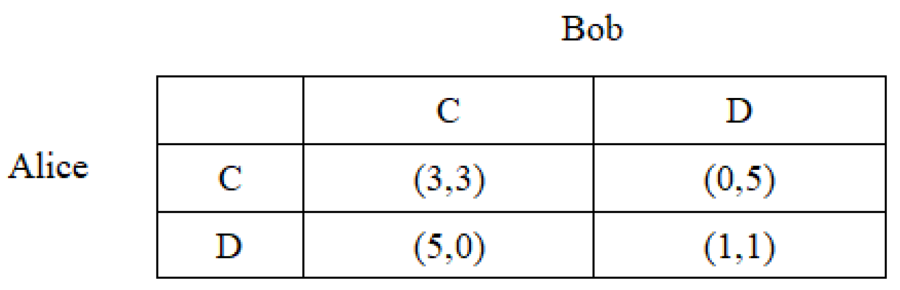
In this section, we mainly discuss the case of 2-player Prisoner’s Dilemma. The payoff matrix of the two players, Alice and Bob, is given in
Figure 1. To be specific, strategy
C means that the player remains silent, while strategy
D denotes that the player confesses. If both of them choose strategy
C (remain silent), each of them will get the payoff 3; if both of them choose strategy
D (confess), each of them will get the payoff 1. On the other hand, if Alice chooses strategy
C and Bob chooses strategy
D, Alice will get the payoff 0 and 5 will be the payoff of Bob, and vice versa.
Since Alice and Bob cannot communicate with each other, strategy D is the dominant choice for each of them no matter which strategy the other one chooses. In terms of classical game theory, the strategic set is the unique Nash equilibrium of the game and each of the two players will get the payoff 1.
In what follows, we firstly focus on the separated quantum game, i.e.,
in (2), which results in
. Assume that the initial state is
Alice chooses the quantum strategy
, and Bob chooses the classical strategy
D, which can be represented by
, i.e.,
. After time evolution, the final state can be calculated as
By the expected payoff given in (5), one can obtain the payoff of Alice
Clearly, Alice will choose to maximize the payoff, which corresponds to the quantum strategies or . As a result, Alice also swaps the initial state and choose the strategy , which leads to the classical Nash equilibrium . Indeed, even if both of the two players choose the quantum strategy (3), all the resulting Nash equilibria are the same as the classical strategic set .
On the other hand, we turn to the maximum entangled case, i.e.,
in (2). In this case, both Alice and Bob choose the same strategies as the separate quantum game above. After time evolution, the final state is given by
By the expected payoff given in (5), the payoff of Alice is given by
Consequently, Alice will choose
to maximize the payoff, which leads to the quantum strategy
. Considering the symmetry of the game,
is also the optimal strategy for Bob. Thus,
is a Nash equilibrium in the maximally entangled case and
Notice that no improvement of the payoff can be made by deviating from the strategic set , which yields a “Pareto optimum”.
4. The 3-Player Prisoner’s Dilemma
In this section, we consider the case of a 3-player Prisoner’s Dilemma. Alice, Bob and Colin are separated and cannot communicate with each other. The strategies
C,
D mean that the player remains silent and confesses, respectively. The payoff matrix [
18] of the three players is given with three numbers in triplets. The first number in the parenthesis denotes the payoff of Alice, the second number denotes the payoff of Bob, and the third one denotes the payoff of Colin. To be specific, if they all choose the strategy
C, each of them will get the payoff 3, i.e.,
; on the other hand, if they all choose the strategy
D, each of them will get the payoff 1, i.e.,
. Moreover, if one of them chooses the strategy
C and the others choose the strategy
D, the former will get the payoff 0 and the latter will get the payoff 4, e.g.,
(or
,
); if one of them chooses the strategy
D and the others choose the strategy
C, 5 is the payoff of the former and 2 is the payoff of the latter, e.g.,
(or
,
).
Again, the dominant strategy for each of them is still the strategy D, i.e., choosing “defect” is better than “cooperate” to earn more payoff no matter what strategies the other two players choose. Due to the symmetry of the game, the strategic set is a Nash equilibrium. However, it is obviously not a “Pareto optimum”. In what follows, we introduce the quantum strategy and investigate the payoff of each player.
4.1. The Separated Case
In this section, we firstly consider the separated case, i.e.,
. Assume that the initial state is given by
and both Bob and Colin choose the strategy
. For comparison, Alice chooses the quantum strategy
. After time evolution, the final state can be calculated as
According to the payoff matrix given in the 3-player case, the payoff of Alice is given by
Thus, it is better to choose for Alice to maximize the payoff, which corresponding to the strategy or . As a result, the total game attains a Nash equilibrium , which is not a “Pareto optimum”.
4.2. The Entanglement Parameter
If
in (2), then the payoffs of all players are connected by the entanglement gate. In this section, we firstly investigate the maximal entanglement parameter by considering the payoff of Alice. The initial state is fixed to be
where the entanglement gate is given by (2) with
. According to prior knowledge in the 2-player Prisoner’s Dilemma discussed above, it has been concluded that both
and
can be used to swap the initial state
and choose the strategy
. However, only
can make the game reach a “Pareto optimum” in the maximum entangled case. In this section, the strategic sets are respectively denoted by
and
for comparison. Then the final state of the game can be calculated by
which yields the corresponding payoffs of Alice for the two cases
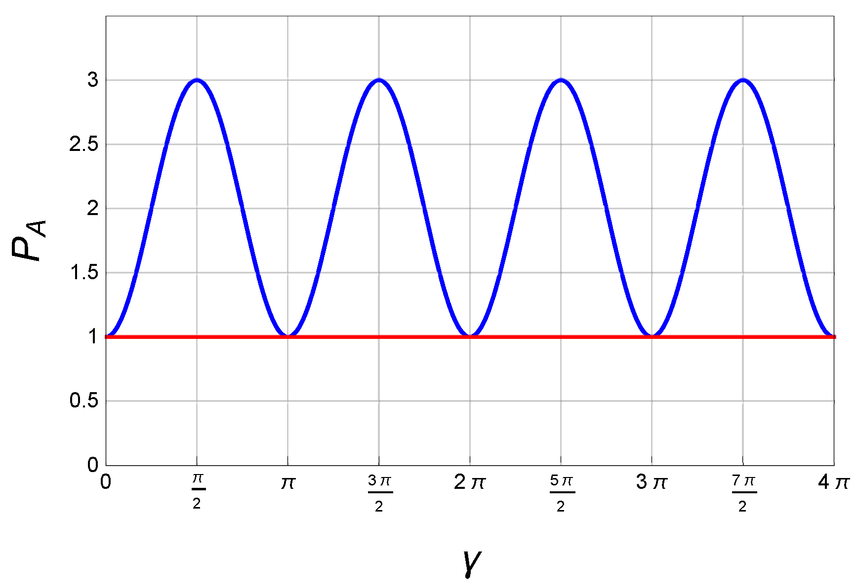
In
Figure 2, the payoffs of Alice with the two strategic sets are simulated. It can be confirmed that
is the optimal strategic set, which enables the game to attain a “Pareto optimum”. Moreover, the maximal entanglement parameter
is not unique. In
Figure 2, the payoff oscillates periodically and reaches its maximum at
,
. In what follows, we mainly discuss the “Pareto optimum” of the game based on two initial states (
and
) with the maximally entangled gate, e.g.,
.
4.2.1. The Initial State
Assume that the initial state is given by
and the maximally entangled gate is
Alice chooses the quantum strategy
, while Bob and Colin choose the strategy
. After time evolution, the final state is given by
According to the payoff matrix given in the 3-player case, the payoff of Alice is given by
Thus, it is better to choose
,
for Alice to maximize the payoff, which corresponding to the strategy
. Similarly, in the case where other two players choose the strategy
, the maximum payoff of Bob and Colin can be derived as
Due to the symmetry property of the game, it can be verified that the optimal strategic set is . In this case, the total game reaches a Nash equilibrium , which is also a “Pareto optimum”.
4.2.2. The Initial State
For comparison, in this section we assume that the initial state is given by
and the maximally entangled gate has the form (20). All of the three players choose the same strategies as the case discussed above, that is, Alice chooses the quantum strategy
, while Bob and Colin choose the strategy
. After time evolution, the final state is given by
According to the payoff matrix given in the 3-player case, the payoff of Alice is given by
Thus, it is better to choose
for Alice to maximize the payoff, which corresponding to the strategy
. Similarly, when the other two players choose the strategy
, the maximum payoff of Bob and Colin can be derived as
However, if all of the three players choose the quantum strategy , the total game attains at a Nash equilibrium , which is not a “Pareto optimum”. Consequently, any player choosing is not a proper way to obtain a Nash equilibrium for the maximally entangled game. Therefore, in what follows we focus on the case of the other two players choosing the strategy , instead of .
4.3. The Case of the Other Two Players Choosing
Firstly, we assume that the initial state is
, and Alice chooses the quantum strategy
, while Bob and Colin choose the strategy
. After time evolution, the final state is given by
According to the payoff matrix given in the 3-player case, the payoff of Alice is given by
Thus, Alice will choose
,
to maximize the payoff, which corresponding to the strategy
. Indeed, in the case of the other two players choose the strategy
, the payoff of Bob and Colin can be calculated as
As a result, all of the three players will get the payoff , which is a Nash equilibrium and also a “Pareto optimum”.
Secondly, we assume that the initial state is
, and Alice, Bob and Colin choose the same strategy as the discussions above. After time evolution, the final state is given by
According to the payoff matrix given in the 3-player case, the payoff of Alice is
Thus, Alice will choose
to maximize the payoff, which yields the strategy
. Moreover, it can be verified that
Consequently, the total game will attain at the Nash equilibrium . In sum, when the initial state is , we can obtain the optimal strategic set no matter whether the other two players initially choose or , which yields a “Pareto optimum” . However, when the initial state is prepared as , we can only get a Nash equilibrium . That is, the optimal strategic set depends on the initial state of the game.
4.4. The Entanglement Gate
Based on the discussions above, it can be observed that the strategic set
is invalid to get a “Pareto optimum”
with the entangled gate
In this section, we aim to seek another entangled gate, which can keep the optimal strategic set to be
and yield a “Pareto optimum”
under the initial state
. In what follows we assume that the maximally entangled state is changed to be
On the one hand, if Alice chooses the quantum strategy
, while Bob and Colin choose the strategy
, then the final state after time evolution is given by
According to the payoff matrix given in the 3-player case, the payoff of Alice is given by
Thus, Alice will choose , to maximize the payoff, which corresponding to the strategy . Due to the symmetry among the three players, the inequalities (23) also hold, which means that is the optimal strategic set.
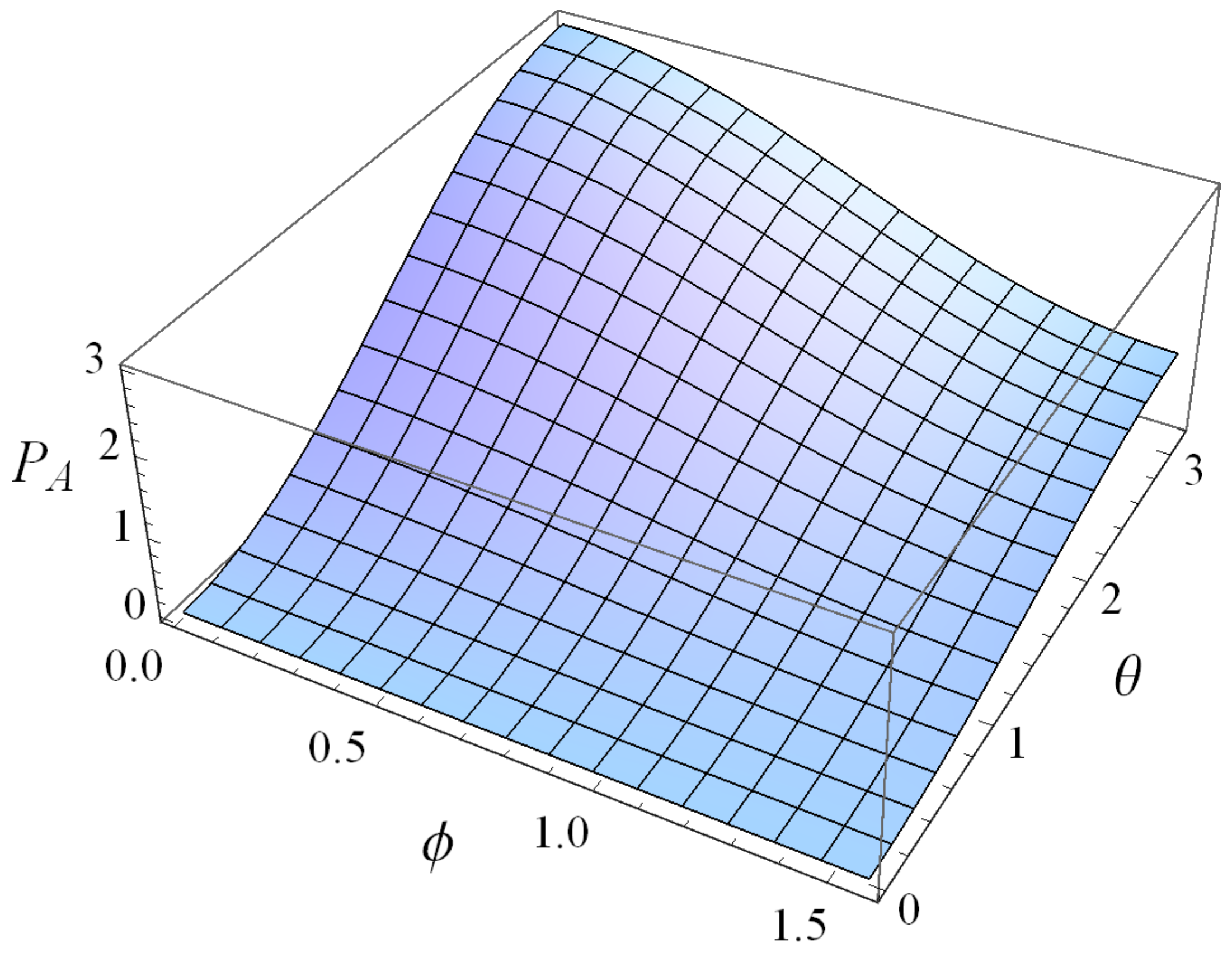
On the other hand, if Alice chooses the quantum strategy , while Bob and Colin choose the strategy , then the payoff of Alice can be calculated in a similar way. Moreover, the inequalities (30) hold in this case.
In fact, no matter Bob and Colin initially choose the strategies
or the strategy
, Alice will persist in choosing the strategy
to maximize the payoff under the entangled gate
with the initial state
, see
Figure 3.
Consequently, when the initial state is prepared as , we can still choose the strategic set to get the “Pareto optimum” of the game by introducing another different maximally entangled state (35).
In this section, a comprehensive study for the 3-player Prisoner’s Dilemma has been presented, which exhibits some interesting features. It should be noted that once the parameter in (5) is fixed, the payoff of player , , in the N-player Prisoner’s Dilemma can be solved by (6). As a result, those features can be generalized to the N-player case in a similar way.
5. Conclusions
In this paper, the general form of N-player Prisoner’s Dilemma in the quantum game theory has been derived explicitly, and yields the payoff of each player under the range of strategic choices. In addition, we have illustrated the advantages of quantum strategy in game theory by introducing the 2-player and 3-player cases. The entanglement parameter is proved to be non-unique, which can be used to obtain the “Pareto optimum” of the game. To be specific, the 3-player Prisoner’s Dilemma with different initial states is discussed and it has been found that the optimal strategic set depends on the selection of the initial state.
From the point of view of the players, each of them can choose the optimal quantum strategy to maximize the payoff based on the initial state of the game. Compared with the classical case, the advantages of quantum features in game theory are determined by the entanglement parameter. Moreover, considering quantum games with incomplete information is in the perspective of our future research.


