Applications of the Network Simulation Method to Differential Equations with Singularities and Chaotic Behaviour

Abstract

In this paper, we deal with some applications of the network simulation method (NMS) to the non-linear differential equations derived of a parametric family associated to stated problems by Newton in and others like the parabolic mirror and van der Pol non-linear equation. We underly the efficientcy of the (NMS) method, compare it with Matlab procedures and present figures of solutions of the equations obtained by it on the mentioned problems. Additionally, we introduce also the electric-electronic circuits we have designed to be able of obtaining the solutions of the referred equations.

1. Introduction

In many problems in science and engineering the network simulation method NSM [1] has demonstrated to be very efficient, for instance, in the simulation of the Frenkel–Kontorova–Tolinson model on friction of two sliding bodies [2].

Friction is a phenomenon present in all mechanical devices in which relative displacements happen. There are different cases to be considered. One of them is the dry friction. In this case the main magnitude is the force necessary to keep a sliding body moving at a given velocity from another considered motionless or velocity threshold at which this force is null.

Solutions in the dynamical problem are very sensitive on the parameters involved in the problems. Such parameters are the interaction force amplitude between atoms of the bodies, the stiffness between the atoms and bulk velocity.

Such solutions are a good example of phenomenon where they can be obtained of an approximate way using NSM with a numerical process shorter than other traditional methods offered in the literature.

In this paper we apply the NSM for obtaining numerical solutions of three examples, a parametric family of non-linear differential equations, the problem of the parabolic mirror and the well-known van der Pol equation. Such approach addresses several difficulties like singularities or chaotic behaviours. The solutions are compared with the results obtained by Matlab. Additionally, the NSM can be implemented in a very efficient and open software used in electronic circuit design, called Ngspice, which has the advantage of requiring a short computing times in comparison with other mathematical software.

The design of the network model implies the following steps:

• Select the equivalence between physical and electrical variables;
• Apply the initial and boundary conditions using the appropriate electrical devices.

The open-source free-software called Ngspice, used in circuit design as numerical simulation software, allows us short computing time by a suitable time step from the point of view of convergence which is adjusted continuously.

2. Methodology

The selected problems are a family of differential equations with infinite slope in some points, the differential equation of a parabolic mirror and the differential equation for the behaviour of van der Pol oscillator.

These equations whose solutions are examples of functions setting out singularities and chaotic behaviour and will be useful to check the capacity of the NSM.

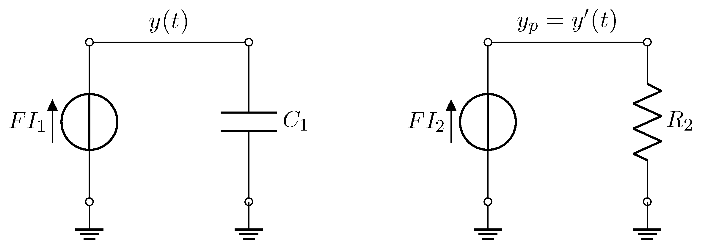
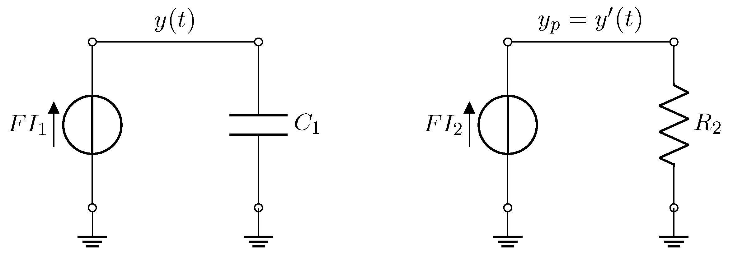
The network simulation method consists in transforming the studied system into electrical circuits with the same governing equations. Physical variables from original system have their equivalent in electrical variables. For example, the variable y in the family of differential equations with infinite slope in some points is equivalent to the voltage in a condenser node, as it will be explained more clearly in the applications of the NSM. Once the circuits equations are solved, using the traditional numerical integration method but with the same efficient techniques used with very-large-scale integration (VLSI), we will have the solution of the physical problem. Only it is necessary to consider again the equivalence between the electrical and the physical variables. Thus, the NGSpice software allows us to simulate electric circuits and analyse the response of them.

In the works of Solano et al. [3] there is a more detailed description of the precision of the NSM in some cases where it is difficult to get the convergence. The equivalent electrical network used for this method is solved by Kirchoff’s laws and a convenient time step considering a stable convergence [4,5,6,7]. In the aforementioned paper, the interaction between the parameters called relative tolerance and chaotic behaviour of the system is analysed. As results of that study the solution stability is guaranteed.

The algorithm used by the software reaches the convergence for any iteration k when the following condition is achieved:

$$|v_n^{k+1}-v_n^k|\le RELTOL·V_{n_{max}}+VNTOL$$

(1)

where $v_n$ is the voltage in the node n and

$$V_{n_{max}}=MAX\left(|v_n^{k+1}|,|v_n^k|\right)$$

(2)

These two parameter, RELTOL and VNTOL, are related to the time step. The values of RELTOL and VNTOL is chosen by the user considering his experience from other solved problems or checking the same problem with several values of these parameters. Besides, several works have been devoted to truncation error using PSpice, from which NGSpice comes from [8,9,10].

From the Vladimeresku analysis using circuits with condenser in which the exact solution is available, Forward–Euler (FE) expression is more liable to the value of time step than the Backward–Euler (BE) expression. The criteria used by software as Ngspice is that the Local Truncation Error (LTE) of constitutive equations for each branch must be limited.

The FE expression provides an inappropriate solution when the time step exceeds a certain value related to the capacitance of the condenser, $\tau$, used in the analysed circuit. The voltage in the nodes belonging to the analysed circuit in which the right solution is zero is assessed by BE expression as a value which decreases over time. On the other hand, the Trapezoidal (TR) procedure provided a solution which oscillates with a decreasing amplitude around zero if time step is greater than $2\tau$. The time constants associated to the electrical networks have time constants utterly different, thus their governing equations define stiff systems. The methods aforementioned must be stiffly stable, that means that the time step can be higher than any time constant of the electrical network. Only the explicit methods are not stiffly stable.

The stability properties of the Gear method with order higher than 1 is good. The simulation provides a solutions according to the selected integration algorithm. The characteristics of Gear and TR algorithms are different despite of the coincidence in the solutions. Speaking about the TR algorithm convergence it was mentioned his oscillatory behaviour. This oscillation is related with the fact that the time step are not smaller than a threshold value. Conversely, the Gear expression of order 2 introduces damping in the solution.

Another advantage of NSM is that it supplies relationships between $y^{\prime }\left(t\right)$ and $y^{″}\left(t\right)$ in cases of second order differential equations. In most cases NSM gives the solutions is easier than other metohds like Matlab. In order to obtain the solution by numerical methods of a second-order differential equation like Runge–Kutta, the second-order equation must be transformed into a system of first-order equations with the difficulty that this implies.

3. Examples of Applications of NSM

3.1. A Family of Differential Equations

We are interested in the analysis of solutions of the components of the following family of differential equations depending on a non negative real parameter a. Some of them are formulations associated to problems stated by Newton on the movement of bodies in the space [11].

In the family, there is a common map $F(t,y)=t/(1-y)$ plus a parameter a. Such parameter increases the slopes of the curves which represent the solutions.

$$\left\{\begin{array}{cc}{y}^{\prime }\left(t\right)=a+\frac{t}{1-y\left(t\right)}=a+F(t,y\left(t\right))\hfill & a\ge 0\hfill \\ y\left(0\right)=0\hfill \end{array}\right.$$

(3)

$F(t,y(t\left)\right)$ is a real analytic function defined in the open rectangle:

$$R(t,y)=\left\{\right(t,y):0<t<1,0<y<1\}$$

(4)

and for $\left|y\right(t\left)\right|<1$ it is $\frac{t}{1-y\left(t\right)}=1+t(1+y\left(t\right)+y{\left(t\right)}^2+\cdots +\cdots +y{\left(t\right)}^n+\cdots )=1+t{\sum }_{n=0}^{\infty }y{\left(t\right)}^n$.

When $a=0$ the equation

$$\left\{\begin{array}{c}{y}^{\prime }\left(t\right)=\frac{t}{1-y\left(t\right)}\hfill \\ y\left(0\right)=0\hfill \end{array}\right.$$

(5)

is the unique of the family which can be integrated by the separation variables method obtaining the unicity of solution for real analytic functions by application the Cauchy theorem on existence and unicity of solutions [12]

$$\begin{array}{cc}\hfill y_0\left(t\right)=1-\sqrt{1-t^2};& 0\le t\le 1\end{array}$$

(6)

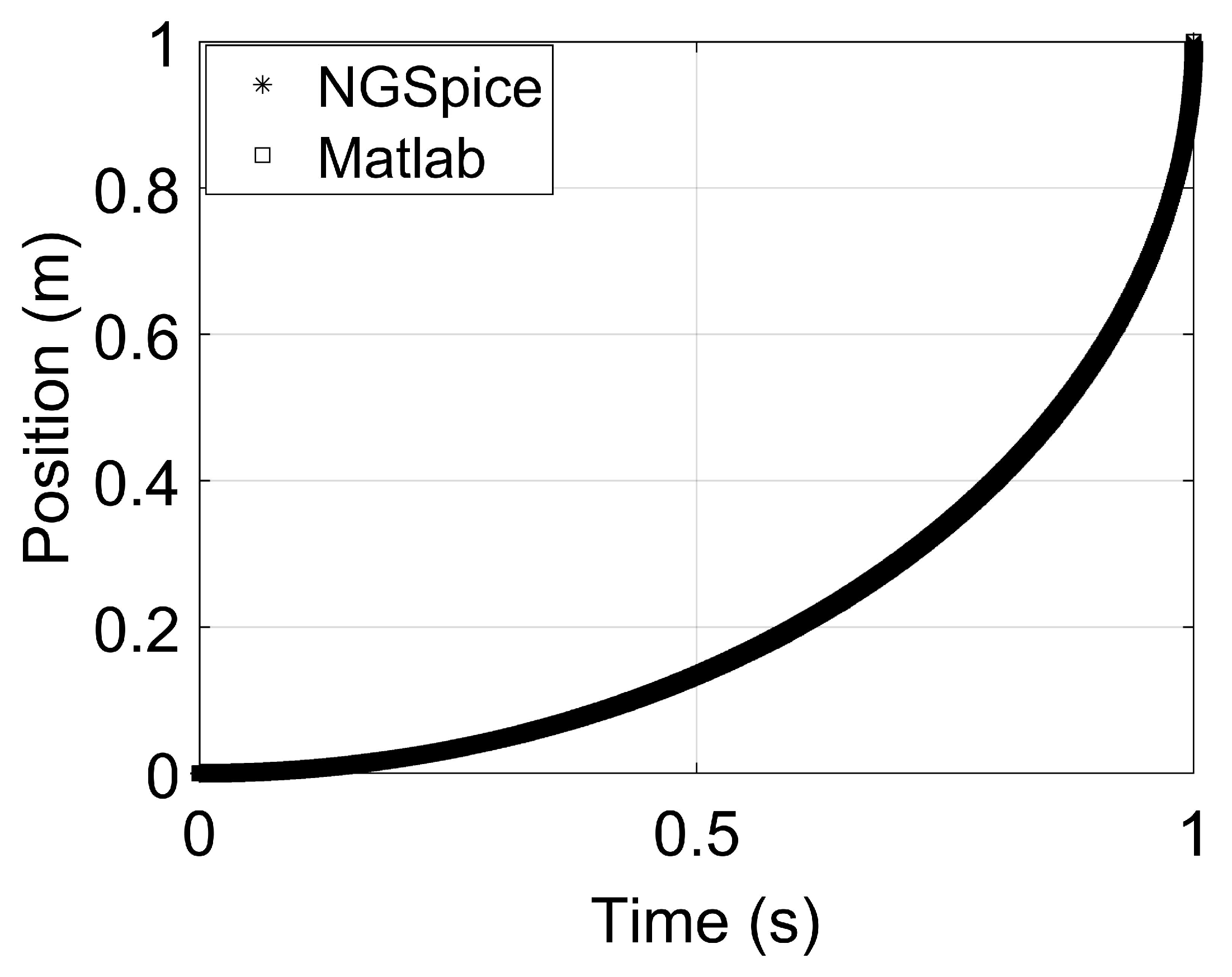
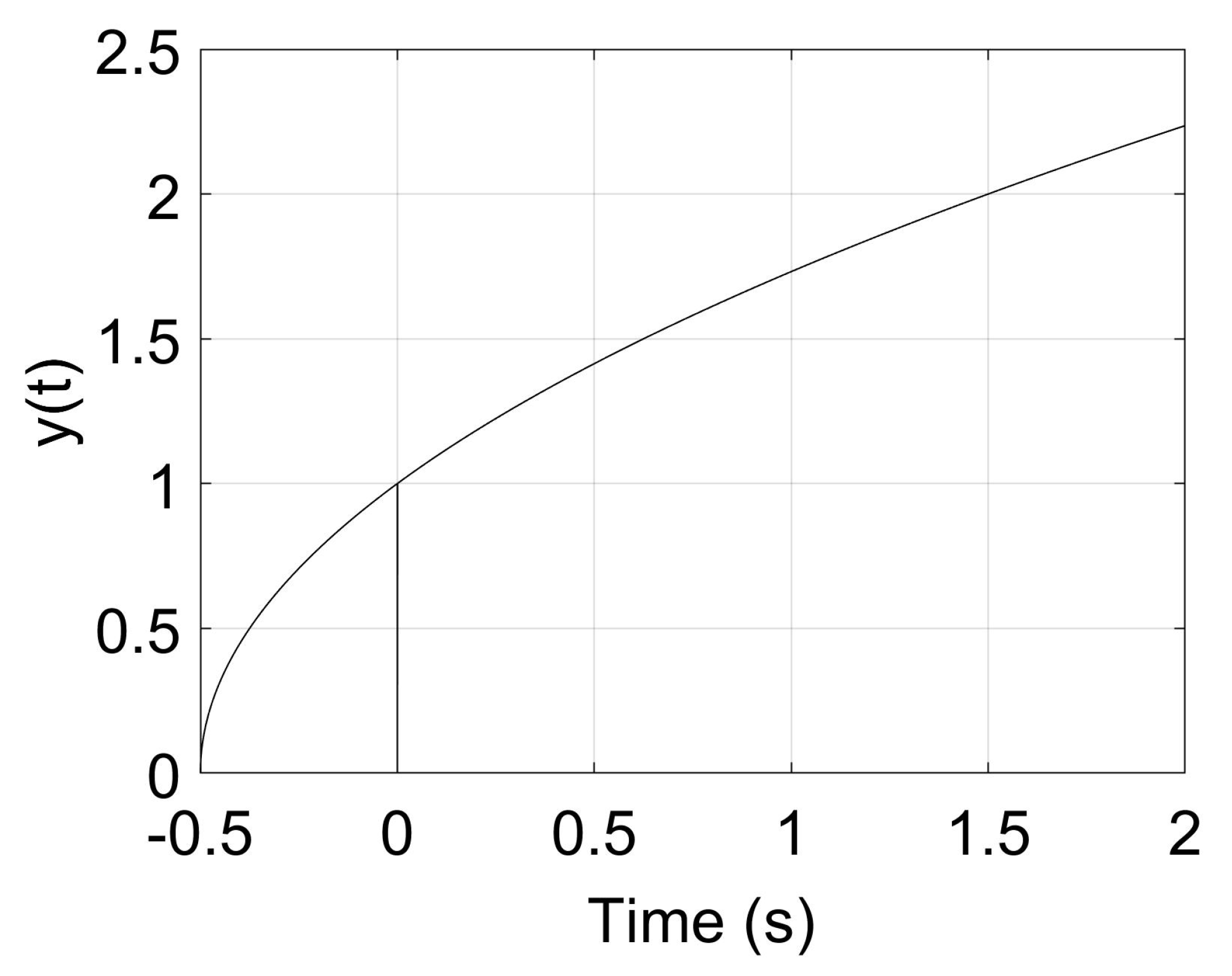
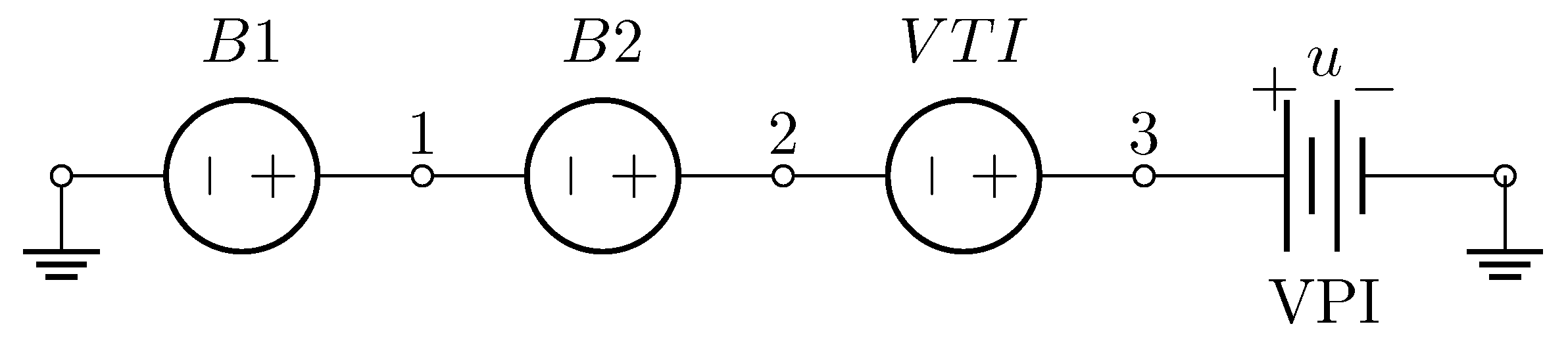
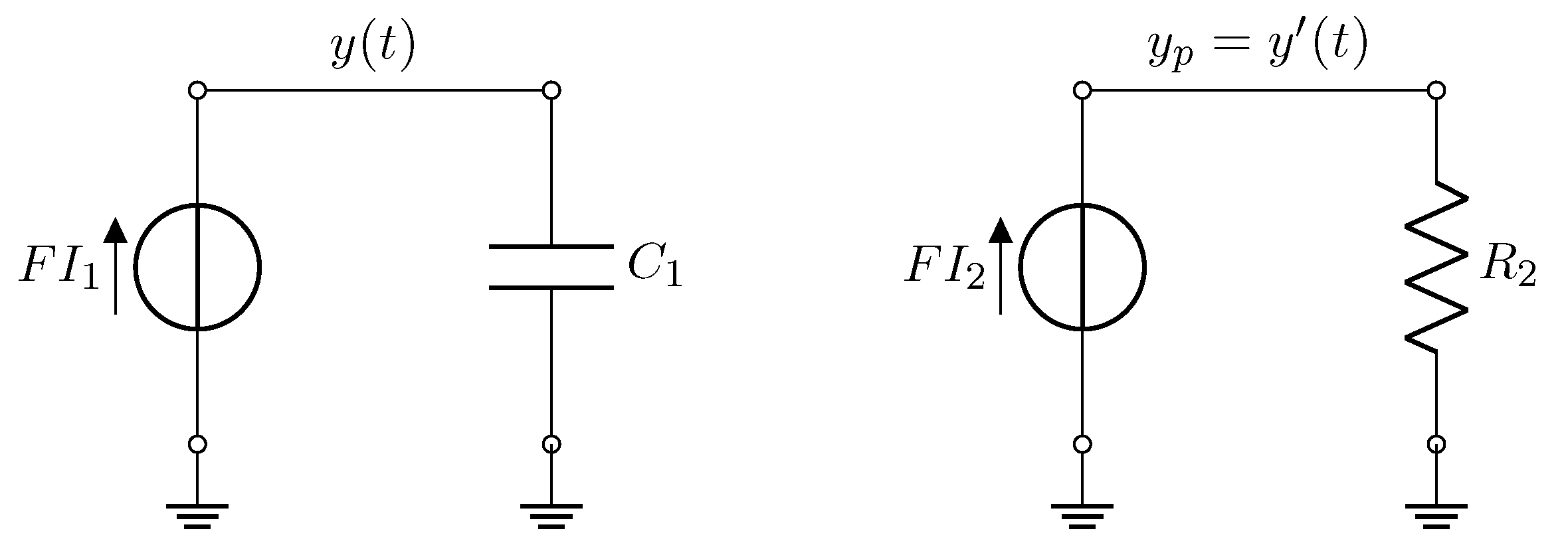
Figure 1 shows this solution where two methods NSM and Matlab, give the same graphic $y\left(t\right)$ for $t<1$. The circuits designed for NSM are represented in Figure 2 and Figure 3.

When $a>0$ it is not possible the explicit integration of such equations. However, the use of power series allows us to solve all cases. Such approach was introduced by Newton [13].

Solutions for $a>0$ are given in the following result where with $y_a\left(t\right)$ we denote the solution for each a:

Theorem 1.

Let $a>0$ in the family (3). Then for every a there exists a unique solution of the equation in the interval $(0,t_a)$ which is real analytic in the same interval where $y_a\left(t_a\right)=1$.

Proof. 

Since $F_a\left(t\right)=a+\frac{t}{1-y\left(t\right)}$ is real analytic in the rectangle set $S_a(t,y)=\{(t,y):0<t<t_a,y<1\}$ using the theorem of Cauchy [12], for each $a>0$ there is unique solution which is real analytic. Then: $y_a\left(t\right)={\sum }_{i=0}^{i=\infty }{a}_i{t}^i$ where $a_i>0$ are real numbers and the power series is absolutely convergent.

The coefficients $a_i$ can be obtained recursively if we have obtained $y_a\left(t\right),y_a{\left(t\right)}^2,$$\dots ,y_a{\left(t\right)}^n,\dots$ For this we are using the Cauchy product of series.

In fact, we have

$$y_a{\left(t\right)}^2=\sum _{i=0}^{i=\infty }{p}_i{t}^i$$

(7)

where

$$\begin{array}{ccc}\hfill p_i=a_0{a}_i+a_1{a}_{i-1}+\dots +a_i{a}_0& and& i\in \mathbb{N}\hfill \end{array}$$

(8)

and

$$\begin{array}{ccc}\hfill y_a{\left(t\right)}^m=y^{m-1}\left(y\left(t\right)\right)=\sum _{i=0}^{i=\infty }{\left(p_m\right)}_i{t}^i& and& \forall m\in \mathbb{N}\hfill \end{array}$$

(9)

where

$${\left(p_m\right)}_i=a_0{\left(p_{m-1}\right)}_i+a_1{\left(p_{m-2}\right)}_i+\dots +a_{m-1}{\left(p_{m-1}\right)}_0$$

(10)

The recurrence to obtain the above coefficients come from the equality

$$y_a^{\prime }\left(t\right)=a_1+2a_{2}t+3a_3{t}^2+\dots +n{a}_n{t}^{n-1}+\dots$$

(11)

$$y_a^{\prime }\left(t\right)=a+t(1+y_a\left(t\right)+y_a{\left(t\right)}^2+\dots +y_a{\left(t\right)}^n+\dots )$$

(12)

where in the (12) we introduce the series obtained in (9) developing $y\left(t\right)$ in power series with unknown coefficients,

$$y\left(t\right)=a_0+a_{1}t+a_2{t}^2+a_3{t}^3+\dots a_m{t}^m+\dots$$

(13)

In the case of (3) since $y_a\left(0\right)=0$ is $a_0=0$, and using the first derivative:

$$y^{\prime }\left(t\right)=a_1+2a_{2}t+3a_3{t}^2+4a_4{t}^3+\dots \dots +m{a}_m{t}^{m-1}+\dots$$

(14)

On the other hand (3) can be written as

$$y^{\prime }\left(t\right)=a+t(1+y\left(t\right)+y{\left(t\right)}^2+y{\left(t\right)}^3+\dots +y{\left(t\right)}^m+\dots )$$

(15)

if $y\left(t\right)<1$, equalling the last two expressions of $y^{\prime }\left(t\right)$ we obtain relationships among the unknown coefficients, $a_1,a_2,\dots ,a_m\dots$.

After calculating some of them we have for $a>0$

$$a_0=0,a_1=a,2a_2=a_1,3a_3=a,4a_4=a_2+a_1^2,\dots \dots$$

(16)

We have generated the coefficients automatically by using a recurrent method, Figure 4. It is not difficult to see that the coefficients are the components of a sequence of positive real numbers convergent to zero. Therefore, in the interval $(0,y_a\left(t_a\right))$, where $t_a$ is the moment in which y reaches the value 1, the power series $y\left(t\right)$ exists and the same for all its derivatives. The variable $y\left(t\right)$ is increasing in the former interval and since $y^{\prime \prime }\left(t\right)$ is positive the map is convex in the same interval. In $t=0$ is $y^{\prime }\left(0\right)=a$ and ${\lim }_{t\to {\alpha }_a^{-}}\left(y\left(t\right)\right)=+\infty$. □

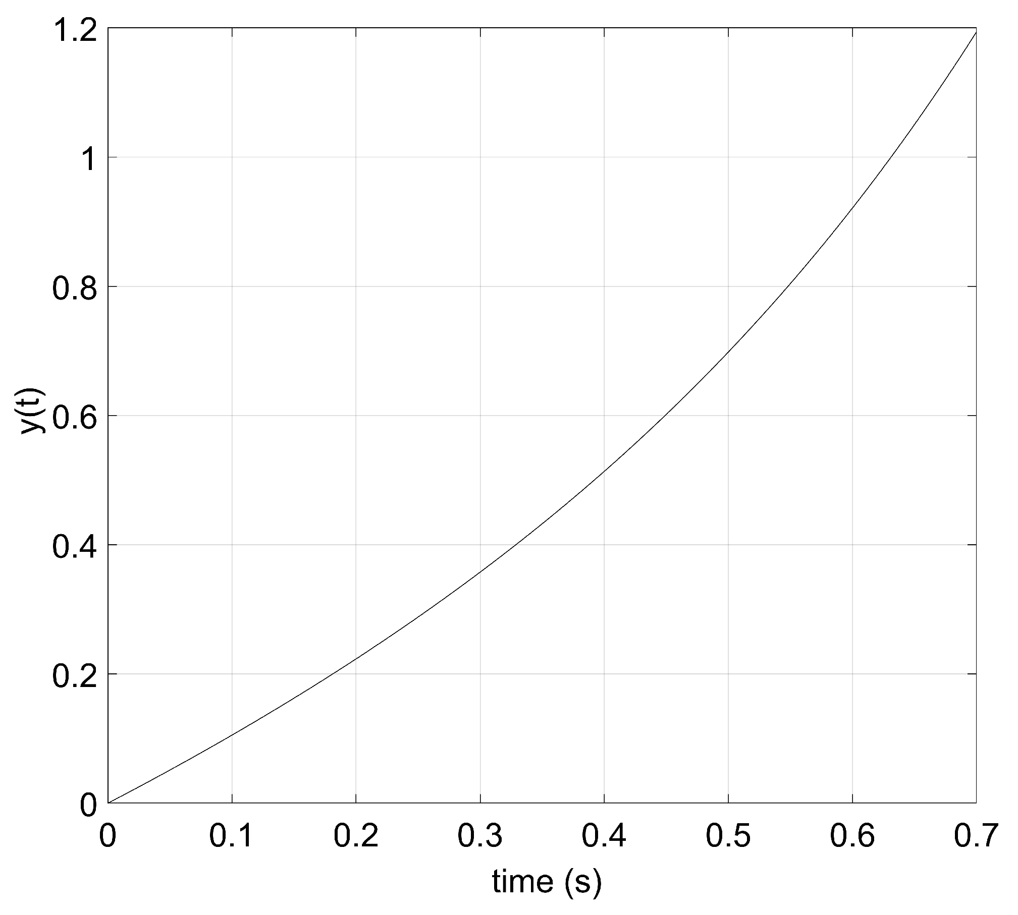
Figure 5 and Figure 6 show the results from, Matlab, and the NSM by Ngspice. The solutions become different for $t>0.5$.

For $t>t_a$ it is not possible to obtain an explicit solution of any equation. Therefore, we have to use numerical approximations to solve it and to study and interpret graphically their behaviour.

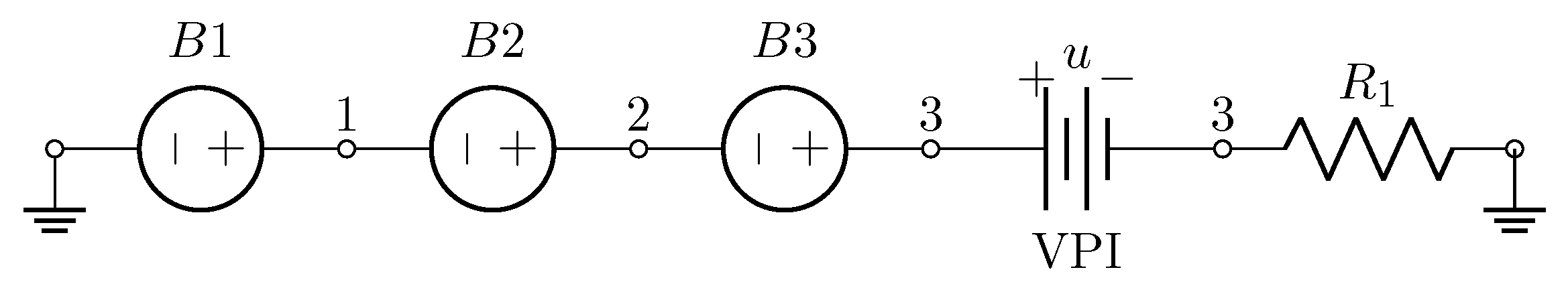
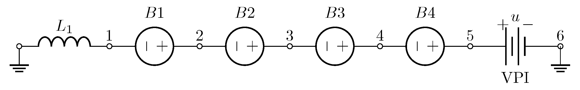
The circuits designed for NSM for this case are represented in Figure 7 and Figure 8.

A particular case of the family (3) is when $a=1$

$$\begin{array}{ccc}\hfill y^{\prime }\left(t\right)=1+\frac{t}{1-y\left(t\right)}& ;& y\left(0\right)=0\hfill \end{array}$$

(17)

When $t\ge t_a$ from Figure 5 we observe the oscillation around $y=1$.

In the interval $(t_a,t_1)$, where $t_1,t_2,\dots ,t_i$ are the times greater than $t_a$ in which the slope of the function $y\left(t\right)$ tends to infinity, the curve is decreasing holding $y_a^{\prime }\left(t_a\right)=-\infty$ and $y_a^{\prime }\left(t_1\right)=+\infty$ and increasing in $(t_1,t_2)$ with $y_a^{\prime }\left(t_1\right)=+\infty$ and $y_a^{\prime }\left(t_2\right)=-\infty$. 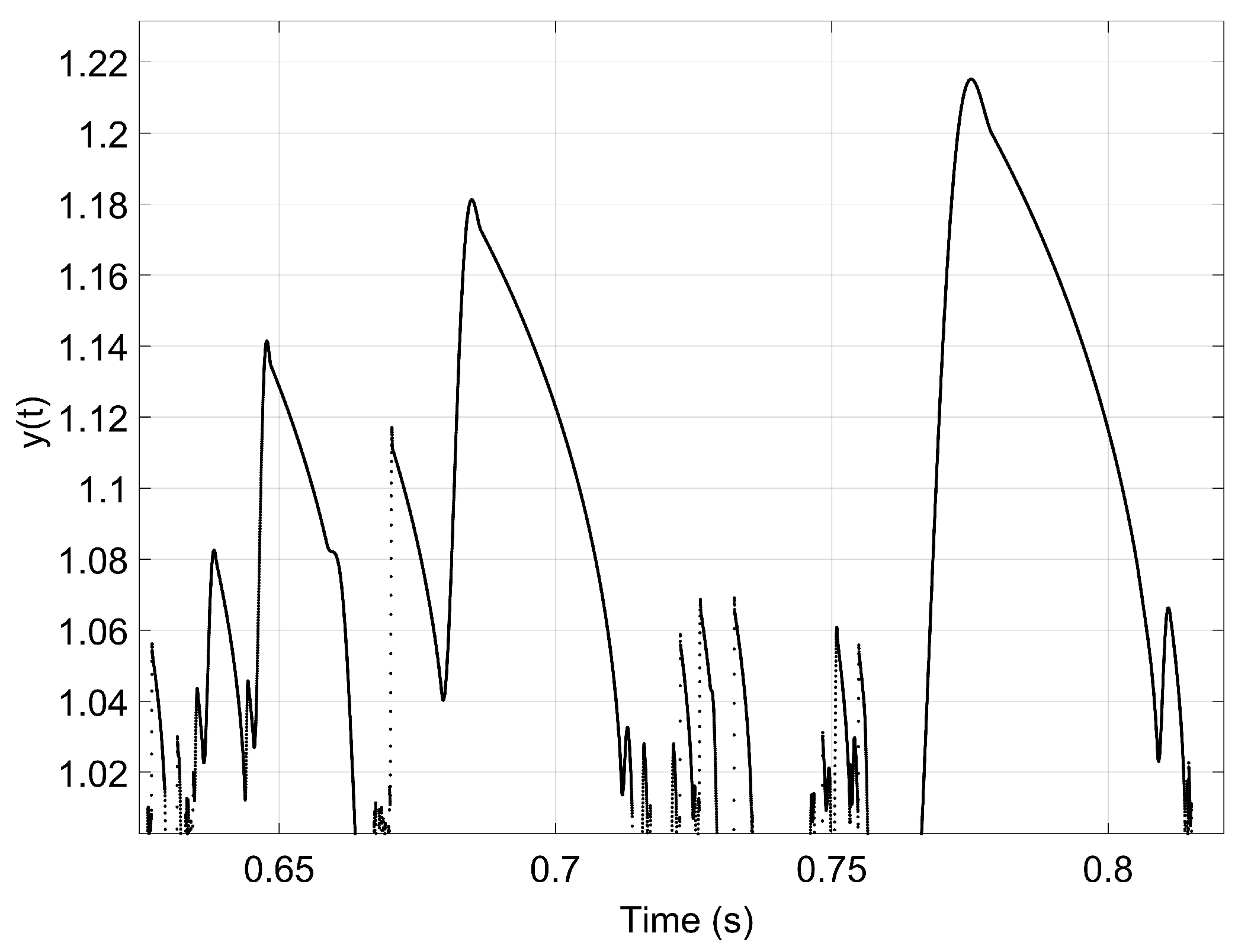The shape of the solution in the interval $(0.5,0.9)$ for Matlab code can be seen in the Figure 9, and in the interval (0.5446, 0.5449) for NSM in the Figure 10. Additionally, in $t_a,t_1,t_2,$ …the curves are non-differentiable. Additionally, in $t_a,t_1,t_2,\dots$ the curves are non-differentiable.

After zooming in on both Figure 9 and Figure 10 the branches obtained by the NSM showing the convexity changes more precise than using Matlab code.

Now we will deal with other properties of the solutions of the equations of the family of differential equations when $t\ge t_a$. In fact, we use the notion of total variation denoted by $V_J$ of a continuous map $f:J\subset \mathbb{R}$ where J is compact. In fact, we follow the definition in the work of Hewitt and Stromberg [14].

$$V_j\left(f\right)={\sup }_{\mathcal{P}}\sum _{i=0}^{n_{\mathcal{P}}-1}|f\left(x_{i+1}\right)-f\left(x_i\right)|$$

(18)

where

$$\mathcal{P}=\{x_0,\dots x_{n_{\mathcal{P}}}\}$$

(19)

is a finite partition of J being $x_0$ and $x_{n_{\mathcal{P}}}$ the extremes of J.

There is a connection between the total variation of a map f and the property of sensitive dependence on initial conditions. It means that if we take $ϵ>0$ and $d=|y_0-y_1|<ϵ$ where $y_0,y_1$ are initial conditions for $t=0$, there exists a $t_{ϵ}$ such that for all $t\ge t_{ϵ}$ the distance d is greater than $ϵ$. The following result can be seen in [15] for discrete dynamical systems on a compact interval of the real line. However, doing simple changes in the statement of the result we adapt the result to differential equations. In fact, we obtain

Proposition 1.

The family (3) depending on a has sensitive dependence on initial conditions and it holds

$${lim}_{t\to \infty }\left(y\left(t\right)\right)=\infty$$

(20)

for every closed subinterval of $[\alpha ,\beta ]$ for $\alpha >t_a$.

3.2. Solution of Differential Equation of a Parabolic Mirror

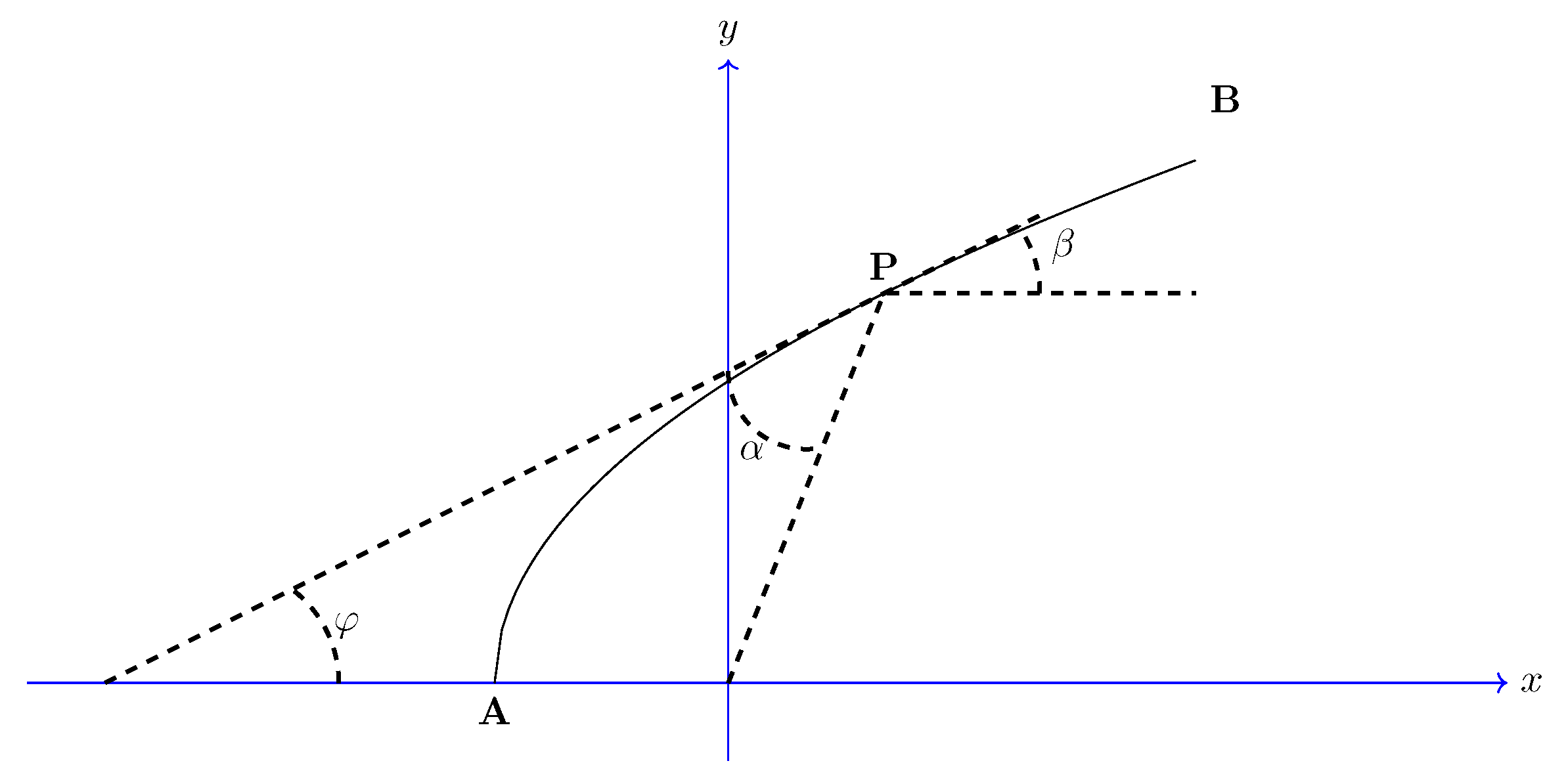
In the well-known book by Newton [11], we can find the definition of parabolic mirror.

By symmetry, such a Mirror will have in space ${\mathbb{R}}^3$ the shape of a surface of revolution generated by rotating an APB curve as indicated in the Figure 11. We can applied the theorem on existence and uniqueness of solutions used in Theorem 1.

The ray that exits with angle $\theta$ exits parallel to the axis $OX$ as indicated in the Figure 11.

From the reflection law, $\alpha =\beta$, as show Figure 11, considering the triangle OFP.

For the geometry of the problem $\phi =\beta$ and $\theta =\alpha +\phi =2\beta$ since $tan\theta =tan\left(2\beta \right)=2tan\beta /(1-{tan}^2\beta )=y/x$, results:

$$\frac{y}{x}=\frac{2y^{\prime }\left(x\right)}{1-y^{\prime }{\left(x\right)}^2}$$

(21)

and solve for $y^{\prime }\left(x\right)$

$$y^{\prime }\left(x\right)=\frac{-x\pm \sqrt{x^2+y{\left(x\right)}^2}}{y}$$

(22)

What is the homogeneous differential equation that verifies the APB curve. Rewriting the (22) in the following way,

$$xdx+ydy=\pm \sqrt{x^2+y^2}$$

(23)

or

$$\pm \frac{d(x^2+y^2)}{dx}=2\sqrt{x^2+y^2}$$

(24)

is $\pm \sqrt{x^2+y^2}=x+c$ with $c\in \mathbb{R}$ and simplifying $x^2+y^2=x^2+2xc+c^2$, it results that

$$y^2=2xc+c^2$$

(25)

it is the equation of all the focus parabolas at the origin and axis $OX$.

Now, we try to solve the (22) with the NSM. In this method, the spatial variable x is replaced by t, the time:

$$2t{y}^{\prime }+y{y\prime }^2-y=0$$

(26)

The software used only provides the solution for $t\ge 0$. In order to obtain the solution for $t\le 0$ it is necessary to turn the curve around the y axis, which is equivalent to multiply t by negative sign. In this way, the (26) is written as

$$-2t{y}^{\prime }+y{y\prime }^2-y=0$$

(27)

or

$$2t{y}^{\prime }-y{y\prime }^2+y=0$$

(28)

Figure 12 and Figure 13 shows the electrical circuit equivalent to the Equations (27) and (28).

If we turn around the Y axis, the solution from the corresponding circuit and call x to t, the Figure 14 is obtained.

3.3. Van der Pol Equation

The well-known differential equation of van der Pol oscillator without considering excitation force is:

$$y^{″}\left(t\right)-a(1-y{\left(t\right)}^2)y^{\prime }\left(t\right)+y\left(t\right)=0$$

(29)

where $a>0$.

The equation for the same system considering sinusoidal excitation force is:

$$y^{″}\left(t\right)-a(1-y{\left(t\right)}^2)y^{\prime }\left(t\right)+y\left(t\right)=Asen\omega t$$

(30)

where $a=8.53$ is a typical value in the literature. For a detailed treatment of Equations (29) and (30) see [16].

We apply a theorem of existence and uniqueness to see that the equation fulfils the theorem. Now, only numerical approach to solution is possible to be done. That is why we directly apply the NSM method.

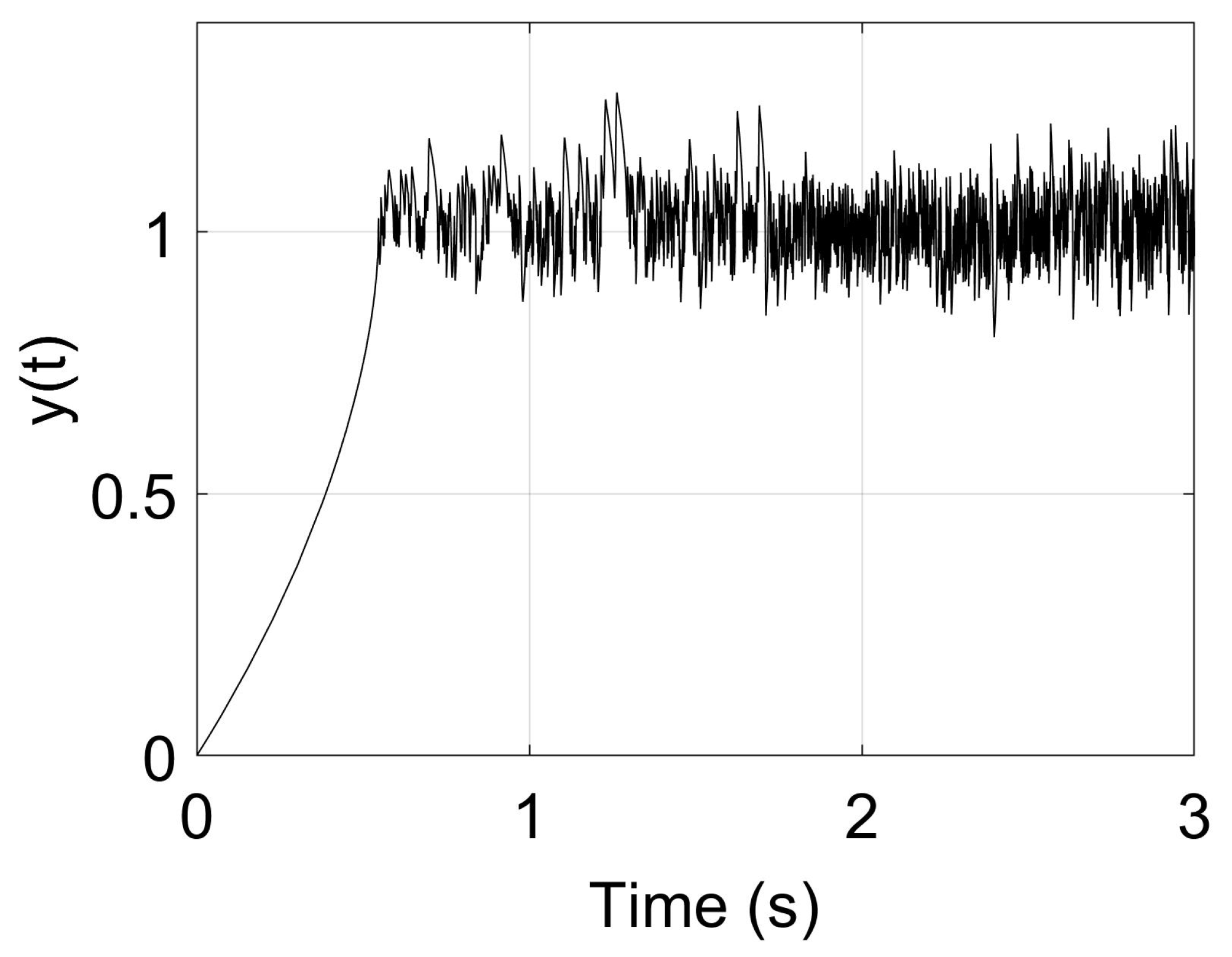
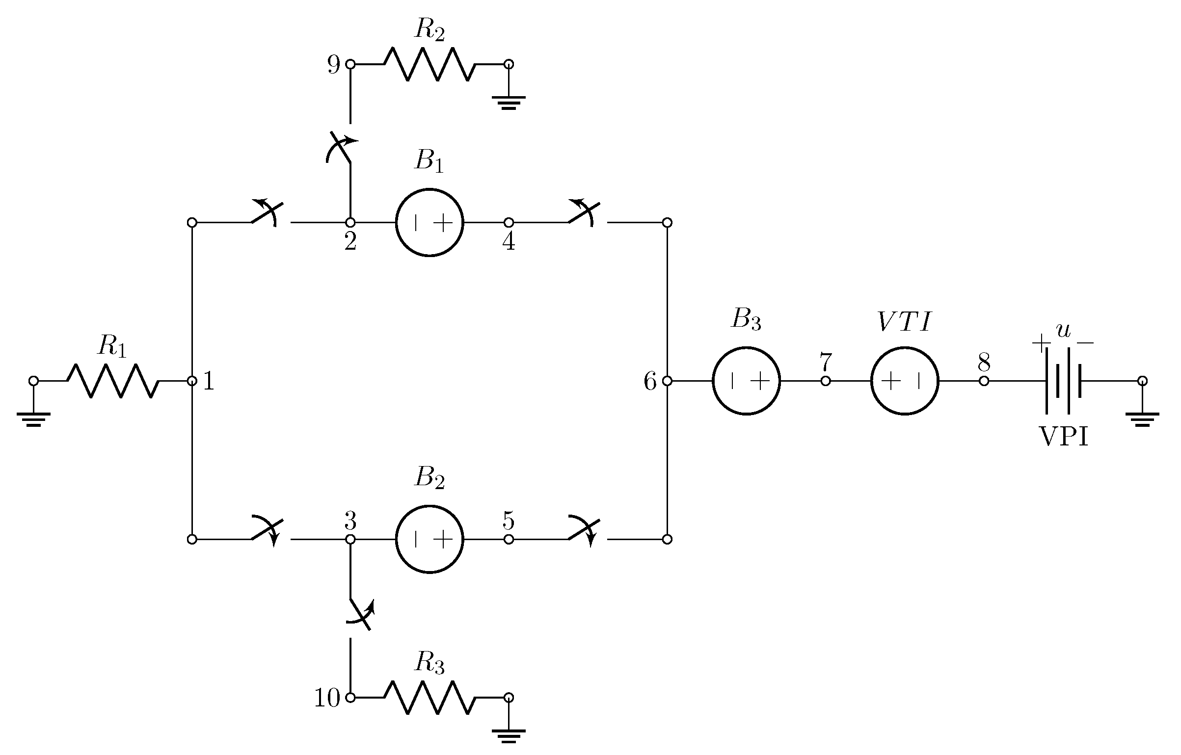
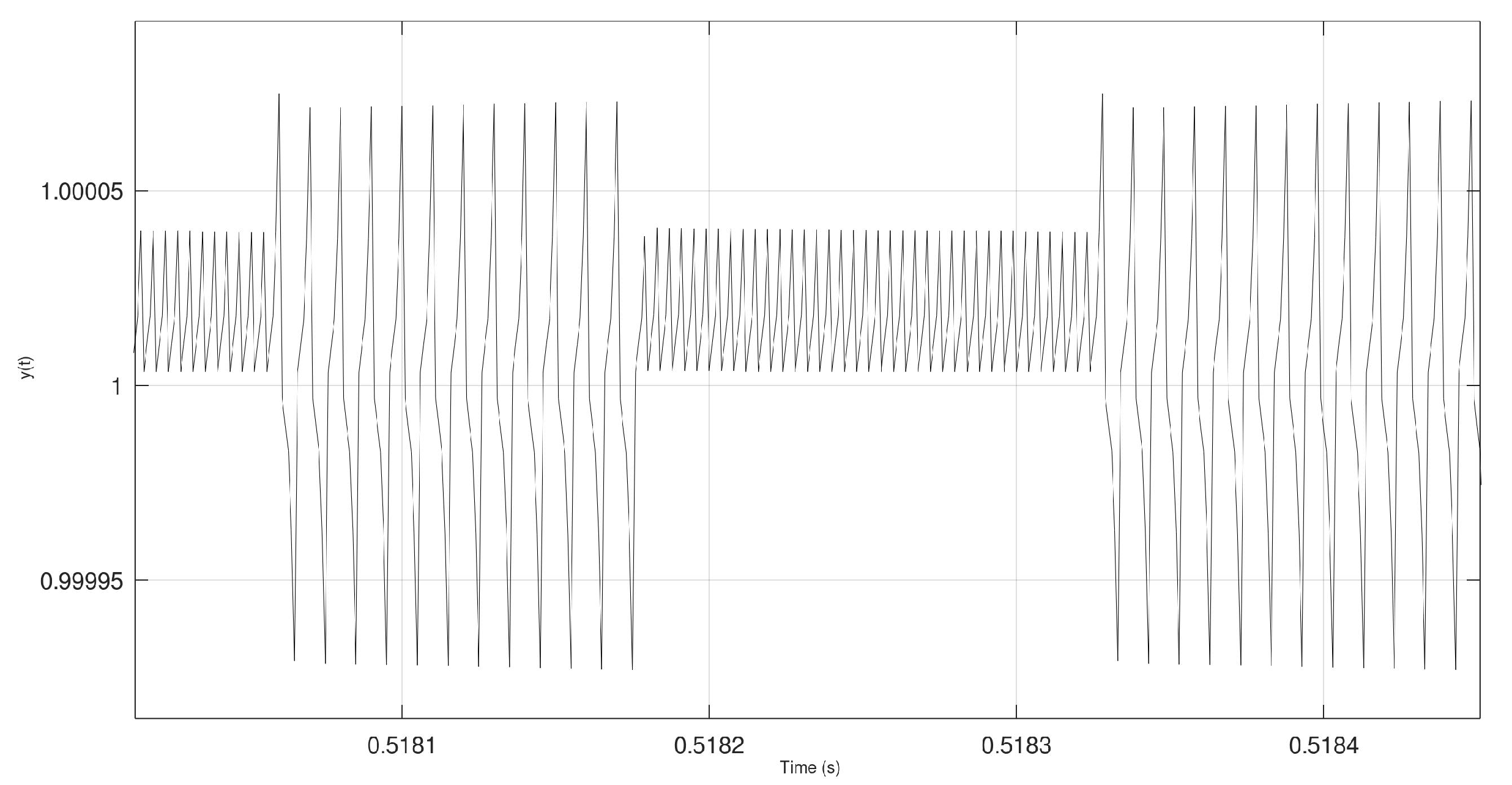
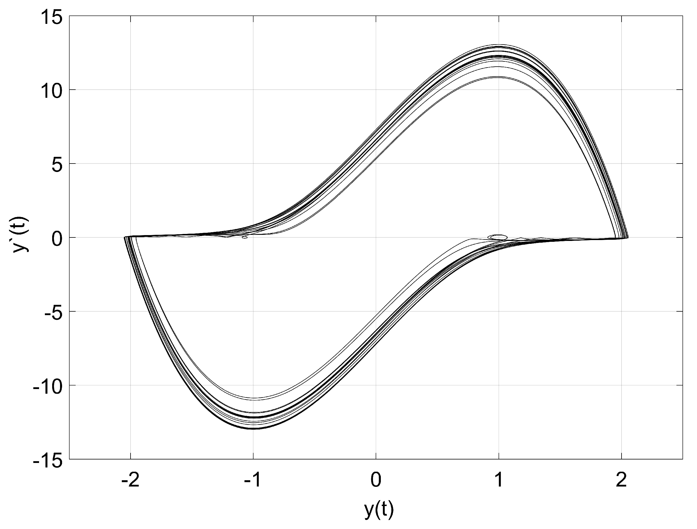
In this case, the designed network for (30) is shown in Figure 15 and the solution in Figure 16 and Figure 17. For $a>1$ the equation is stiff. In Figure 16, we appreciate the typical oscillations of solutions up and down of $y=0$.

4. Conclusions

The former examples show the capacity of the NSM to address equations with some singularities or chaotic behaviour like the mentioned family of differential equations. Besides, the use of this method in case of system of equations can be implemented with more easiness as other methods because it is only necessary to copy the networks already designed with the only care to change the denomination of each network.

Additionally, it can be implemented also for solving non-linear systems of differential equations.