
The Influence of Transport Link Density on Conductivity If Junctions and/or Links Are Blocked


Department of Systems Management and Modelling, MIREA—Russian Technological University, 78 Vernadsky Prospect, 119454 Moscow, Russia
Mathematics 2021, 9(11), 1278; https://doi.org/10.3390/math9111278
Submission received: 14 May 2021
/
Revised: 28 May 2021
/
Accepted: 30 May 2021
/
Published: 2 June 2021
(This article belongs to the Special Issue Applied and Computational Mathematics for Digital Environments)
Abstract
:This paper examines some approaches to modeling and managing traffic flows in modern megapolises and proposes using the methods and approaches of the percolation theory. The author sets the task of determining the properties of the transport network (percolation threshold) when designing such networks, based on the calculation of network parameters (average number of connections per crossroads, road network density). Particular attention is paid to the planarity and nonplanarity of the road transport network. Algorithms for building a planar random network (for modeling purposes) and calculating the percolation thresholds in the resulting network model are proposed. The article analyzes the resulting percolation thresholds for road networks with different relationship densities per crossroad and analyzes the effect of network density on the percolation threshold for these structures. This dependence is specified mathematically, which allows predicting the qualitative characteristics of road network structures (percolation thresholds) in their design. The conclusion shows how the change in the planar characteristics of the road network (with adding interchanges to it) can improve its quality characteristics, i.e., its overall capacity.
1. Introduction
Controlling and balancing flows in transport networks is one of the main problems of modern conurbations. Urbanization and the development of the motor transport industry have led to the emergence of huge vehicle flows moving within our current limited traffic infrastructures, and this has led to an increase in delays and, consequently, a loss of time and money, as well as increased emissions of harmful substances into the atmosphere.
All this entails the requirement for traffic flow control and balancing models and methods to be developed. In general, it is necessary to look at the topology of a transport network in order to solve the dynamic task of traffic redistribution. The problem in so doing, however, is that the number of vehicles in the network is constantly increasing and, as a result, current management models become outdated and inefficient. It is, therefore, necessary to search for new management tools or to modernize the physical base (road width and length, number of lanes etc.) of the current transport network. Let us consider some of the current approaches to traffic management in transport systems which fall into two categories: local and systematic management.
Local management is carried out on the basis of statistically estimated vehicle characteristics. The result is provided with the estimate of transport flow efficiency per any single road junction regardless of any neighboring ones. Systematic management provides transport flow optimization in the sphere including many junctions and, as a rule, operates considering the macro-characteristics of the flow. Any change in management operations on any single junction inevitably leads to a change in neighboring transport flow characteristics. Conflict between local and systematic management methods is common. Thus, if a network simultaneously uses both management methods, these should be implemented at different times. Local management time is selected with the aim of limiting the influence of transport flow on neighboring junctions.
Without dwelling in detail on transport flow analysis and the development of management models throughout history (which include models proposed by Grinschields, Richards, Grindberg, El Hozaini, Underwood, Drake, and Pipes: optimal speed, “Smart” driver, leader follow, cellular automata models, etc.) and the different methods of classification, this paper instead presents some more recent models.
For example, in [1], a network flow model based on a conservation hyperbolic system with discontinuous flow was investigated. This investigation showed that the model could be quickly developed because additional procedures were not required for solution management. The model developed enables us to automatically select the solution where a flow is maximized in each direction (user’s optimum), i.e., there is no need to calculate maximum flow, which could be transferred through any junction (global optimum), as the model is developed according to standard approaches.
In [2], the authors developed a short-term traffic forecasting method. During this investigation, an efficiency comparison of specific algorithms was undertaken using the Volterra prediction model, RBFNN (radial basis function neural network). According to such a comparison, the Volterra model was selected where traffic data were normalized to simplify the programming of algorithms.
In [3], the authors developed an algorithm to calculate the exact average speed of flow movement using mobile detector data for measuring movement speed. The algorithm developed indicates average speed on a given road section, ignoring repetitive messages, and a travel time filter is used to compensate such time selection exceeding the road speed limit. Furthermore, this method comprises errors, such as errors caused by connection failure, dubbing recording, and other factors.
In [4], the authors performed an investigation on the calibration and testing of a macroscopic traffic flow model. Their model was investigated and compared to 10 different algorithms in total (regarding its ability to converge to this solution) for different datasets. Optimization algorithms using particle swarm (PSO) seemed to be the most effective in terms of both convergence rate and solution compilation.
In [5], the authors used a Gaussian regression model (GPR), optimized using particle swarm algorithm (PSO), to predict undefined, nonlinear, and complex traffic in a road tunnel.
Other studies [6,7] described models of stochastic flow dynamics in traffic networks with nondeterministic characteristics of statistical parameter distribution, describing the dependence of the probability of blocking individual nodes from traffic characteristics over time. The developed mathematical models describe the rules of intersection maintenance (time of switching traffic lights), considering the material balance of the number of cars in the system and the connection of their flows between neighboring intersections. The authors of [6,7] showed that the use of percolation theory techniques and the results of the stochastic model of traffic flows allows simulating the operation of the transport network at the level of not only individual nodes, but also the whole structure. The proposed model allows using a real map of the transport network to create its dynamic model, as well as simulate its work and the occurrence of traffic jams.
In [8], the authors studied traffic flow instability in experimental and empirical investigations. To calculate traffic instability, the authors considered the competition between stochastic violations, which can tend to destabilize traffic flow, and how drivers adapt to changing speeds, which can, in contrast, tend to stabilize traffic flow.
In [9], the authors developed a modified algorithm for optimizing the transportation route according to street traffic flow. This study was based on a modified ant algorithm (ant colony optimization algorithm), being one of the most effective polynomial searching solutions for dealing with problems regarding route optimization.
In [10], a structural analysis of public transport routes was performed concerning tariffs and operating mode. To provide more adequate and logical results, the advanced route calculation algorithm was proposed for different structures.
In [11], the authors developed a transport network algorithm in the form of a pre-fractal graph based on their theory. The search for solutions to multi-objective problems using an indication of the optimal path was carried out by algorithms which searched for optimal solutions on several criteria if the presence of such criteria was proven or based on a solution with specific deviations from the optimal solution. In this paper, the largest maximal chains extraction algorithm (MCEA algorithm) was used with the arbitrary graph.
In [12], the professional system and regulator using the fuzzy logic module was studied for traffic control systems at intersections.
In [13], the authors developed a traffic control method based on a traffic efficiency index they compiled, comprising factors such as traffic and road capacities.
In [14], the authors studied loaded traffic management issues using a prediction model for any specific intersection and within the transport area. Using a solution based on a predictive management algorithm model, the residual queue is distributed, due to a transport demand which exceeds the capacity of the crossing, along all incoming transport links. Simultaneously, in the case of long-term implementation of the intersection, a big queue accumulation in oversaturation mode is observed. In this case, a network-wide delay can be prevented by decreasing transport demand at intersection entrances only.
Another author [15] studied the possibility to use the main network traffic diagram for prediction of traffic functioning conditions in cities. The traffic model studied by the author was based on the use of standard Pipes model for indication of dependencies between speed and density for traffic performance calculation. The model analysis showed that it is necessary to limit a high level of vehicle accumulation and use the correspondent management strategies when controlling traffic on roads in cities.
In [16], the authors studied the nature of traffic interval distribution depending on the distance from the previous signaled crossing. According to the investigation results, the authors made a conclusion that normalized Erlang distribution is the most suitable practice for description of intervals inside traffic groups.
In [17], the principles of using telecommunications technologies based on the protocols of interaction of the type “car-to-car” were examined to organize an efficient infrastructure in terms of ensuring traffic transport. The information used for this method included the parameters of movement, the location, and the parameters of the state of the car’s systems. After processing and analyzing this information, it is possible to form recommendations and management effects. These recommendations are used by the driver or an automated driving system. The article described a model that allows realizing the interaction of cars, which can determine the optimal use of the car’s resources, as well as the aggressive driving style of the vehicle.
A brief review on the development of recently created models shows that, despite their variety, no investigations studied the general features of transport network structure, indicating its conductivity. No works banded the dynamic characteristics and structural features (topology) of transport systems.
Accordingly, this paper aimed to study the effect of the density of transport network connections on their conductivity when blocking nodes and/or links, analyzing the dependence of such an influence and finding generalized patterns for predicting the properties of the road network (the possibility of determining the percolation threshold based on the calculated density of the road network). This should take into account different types of network structures (planar and nonplanar networks) and various tasks to be solved (node tasks and link tasks).
2. Statement of the Problem
The significant density index of vehicles per area unit of all current roads leads to an inevitable congestion of vehicles at one or other elements of the traffic system (e.g., intersections and roads), i.e., delays (jams). Most traffic investigations, analyses, and subsequent developments of management models focus on local-level solutions, not considering the transport network.
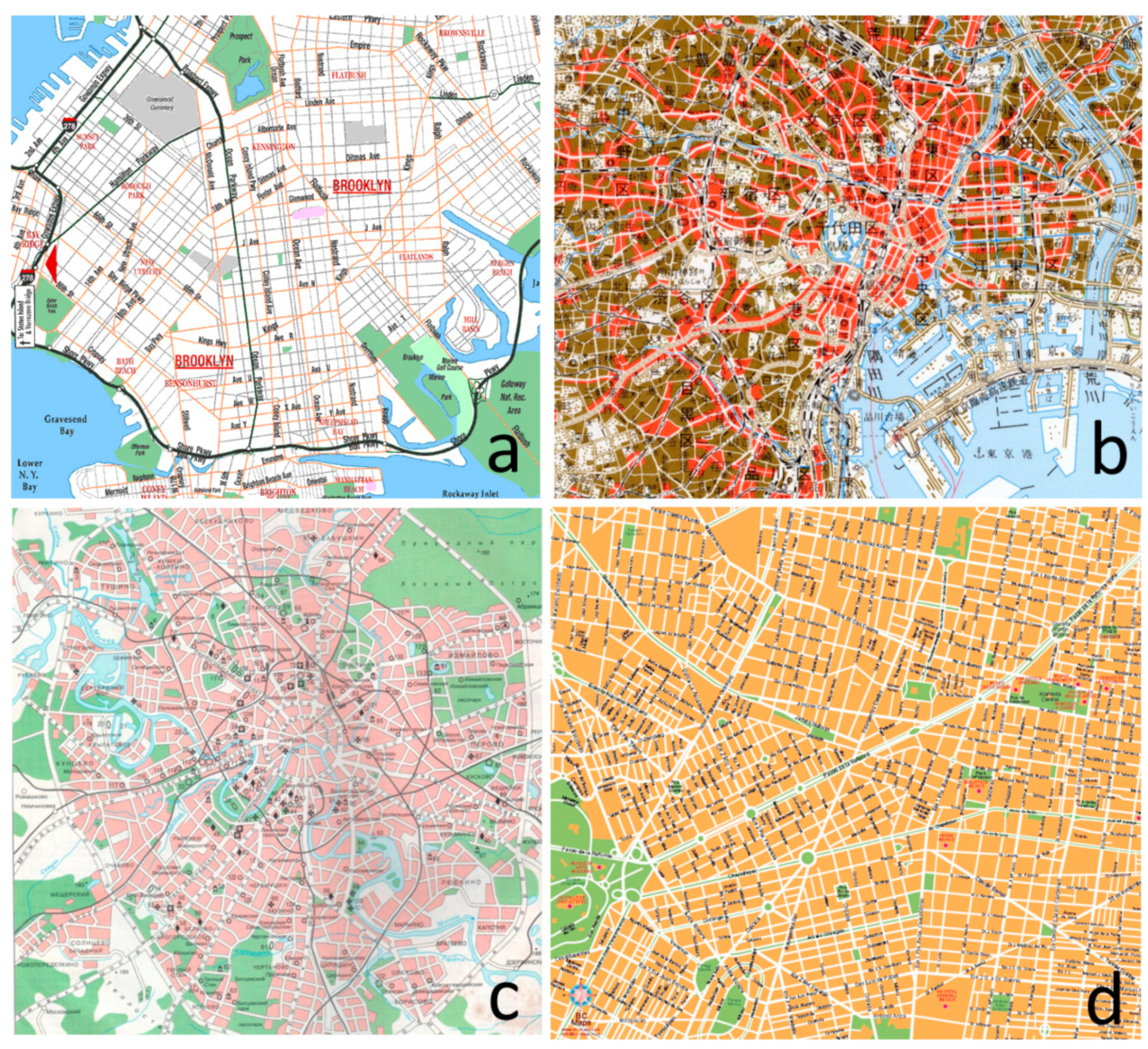
The traffic systems of modern conurbations have very wide, complex, and branching structures (see Figure 1 for example), which may be represented as a graph (junctions—road intersections and edges—roads). When modeling traffic, it is necessary to consider the dynamic of traffic mass change (daily variation of flows) and the fact that all elements of the transport graph (junctions and edges) have different characteristics (traffic capacity).
If we trace the path of the detailed traffic graph model generated with a detailed description of its attributes (number of lanes, route length, number of directions at intersections, etc.), requiring such a model for the local management of traffic would be extremely complicated and difficult to implement for practical purposes.
It is arguably more convenient to create a traffic percolation model to make the structure more efficient, regardless of which specific elements could be blocked due to the formation of traffic delays. In this case, functioning and reliability mean that at least one freeway is possible which comprises unblocked graph elements between any two arbitrary network junctions.
3. Percolation Theory Methods for the Network Transport Structures
Percolation theory (graph-based probability theory) studies solutions to problems relating to junction and link tasks [18,19,20,21] for networks with various regular and accidental structures. When solving the link problem, the link share must be separated by at least two isolated parts (or, conversely, the fraction of conductive nodes (crossroads) when conductivity occurs). When solving junction problems, the fraction of blocked junctions is indicated where the network is broken up into isolated clusters within which links can be kept (or, conversely, the fraction of conductive junctions, when conductivity occurs). Percolation threshold is the fraction of nonblocked junctions (junction task) or unbroken nodes (crossroads) (nodes task), where conductivity occurs between two randomly selected network junctions. For the same structure of percolation threshold values, junction, and nodes (crossroads), tasks have different meanings. Note that, in the case of junction blocking, all links are blocked, and, in the case of node (crossroad) blocking, only one link is blocked between neighboring junctions.
Use of the term “blocked junction fractions” or “blocked road fractions” is equivalent to the occurrence probability that a randomly selected junction (or nodes) will be blocked. Therefore, we may accept that the percolation limit value indicates the probability of passage through the whole network if any of its junctions (or links) are blocked or (removed), i.e., given the average probability of a single junction (or nodes) being blocked.
Achieving the percolation threshold in a network corresponds to a cluster where links exist among random junctions. An endless or contracting conducting cluster is formed. Note that this approach claims to be universal and can be applied not only to the topology of road networks, but also to other topologies [22].
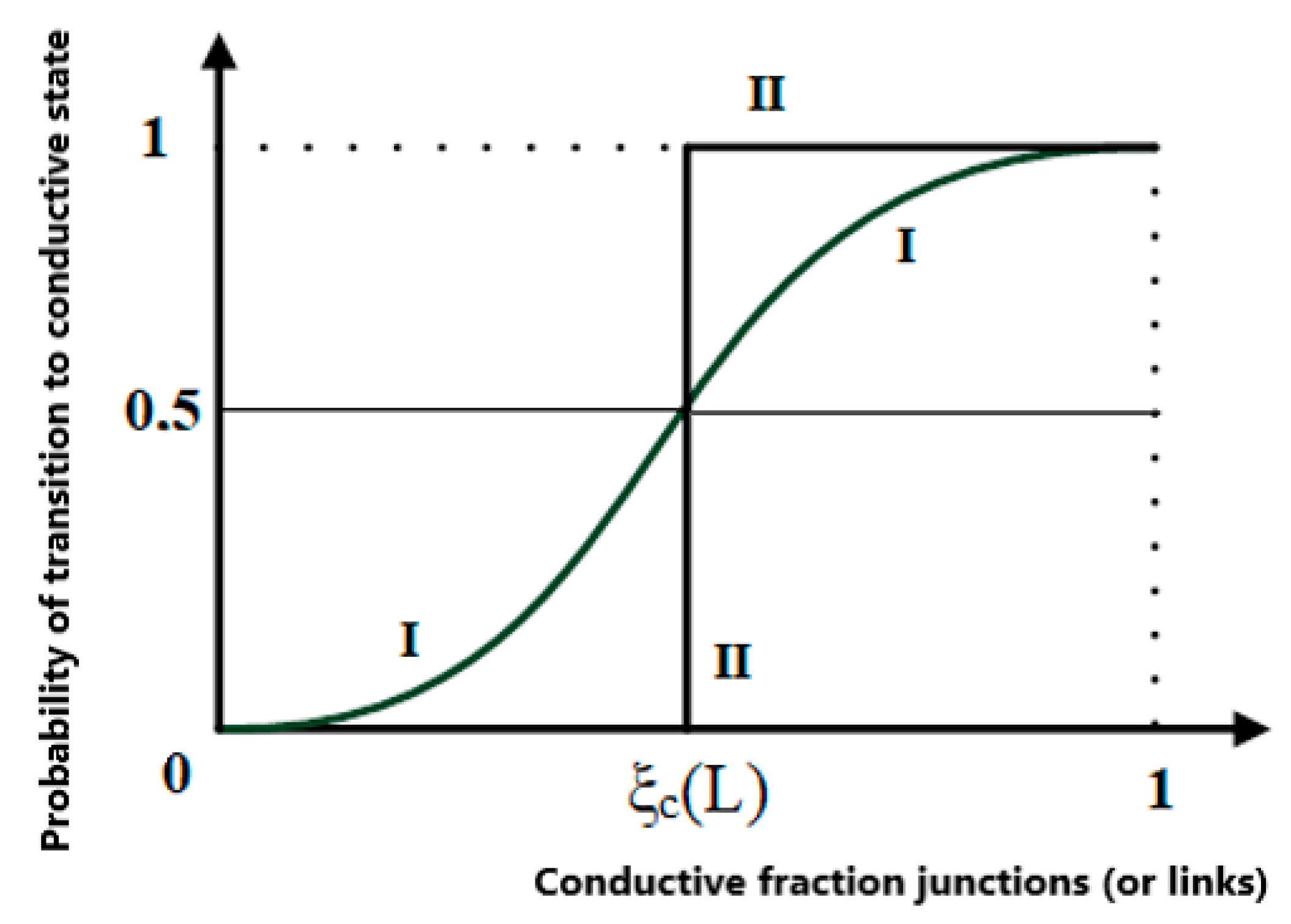
For finite structures, conductivity may appear at different fractions of conducting junctions (or links, see Figure 2). However, if network size L tends toward endlessness, then the sphere of transfer becomes compact (see Figure 2, curve I for small-sized structure or curve II for an endless network).
For finite-sized structures, the percolation threshold structure ξc(L) may be determined from the fixed value of network transition probability in relation to the conducting state. In Figure 2, this probability is chosen to be equal to 0.5 (50%). However, we could also take a value of 0.95 or 0.99, for example (then, the percolation threshold would correspond to the given criteria of network reliability working); in other words, it is possible to determine what fraction of blocked junctions and/or links influences the decrease in the necessary level of performance.
Based on specified work reliability values (the probability of transition or being in conductive state), we can find the fraction of unblocked junctions (or road).
The fraction of blocked junctions (or links) where network conductivity disappears (which can be calculated as follows: one minus conductive junctions (or links)) causes the blocking of the network as a whole, and this value can be associated with the macro-characteristics of traffic in the current transport system. In the simplest case, we can give the following estimate: the accepted level of intensity of traffic without delays (presented as ) for European cities is 600–900 vehicles and in the USA up to 1300 vehicles per hour per lane; in Russian cities, this index is 300–700 vehicles per hour per lane. Therefore, knowing the total city road stretch and number of lanes, as well as daily vehicle dynamics, we can use such data to calculate the average traffic intensity at any moment (presented as ). Then, the average probability () of a network element blocking at any moment in time t may be indicated as follows:
Furthermore, using such a probability estimate of network element blocking, we can find, at a given time t, the state of the reliability and efficiency of the network as a whole, as well as analyze daily dynamics of changes to the network and, consequently, if necessary, change the structure (for example, link density) of the transport system as appropriate (the way in which the traffic functioning reliability is associated with density of its links, for example, as discussed later in the article).
For exact estimates of average blocking probability, different macroscopic mathematical models of traffic flows can be used (drawing on the models proposed by Grinschilds, Richards, Grindberg, El Khozaini, Underwood, Drake, and Pipes: the optimum speed, “Smart” driver, leader follow, cellular automata models, etc.).
The main problem when investigating percolation features of network structures which have accidental structures is that there are currently no established analytical methods and, as such, it is only possible to study such networks by using computer-aided simulation. First of all, it is necessary to build a topological graph, which is itself a rather difficult task for studying the percolation properties of planar network structures which have accidental structures.
The application of some methods of percolation theory to traffic flow modeling was described in [23]. In this paper, traffic dynamics were seen as a critical phenomenon, in which there was a transition between isolated local and global flows on the roads with the formation of clusters of congested sections of the transport network in local structures and their unification into a global cluster. Local flows are connected by narrow links, and narrow links can occur in different places of the transport network at different times of the day. The authors of [23] described such processes as the percolation of traffic between local clusters. The authors tried to describe how local traffic flows interact and merge into a global stream across the city network.
When modeling a transport structure, it is difficult to assess the entire dynamics of traffic organization throughout the network as a whole and to link it to local traffic characteristics. To solve this problem, the authors [23] used the percolation theory. They collected and analyzed the speeds of more than 1000 roads with record 5 min segments measured on roads in Beijing’s central district. The data covered a period of 2 weeks in 2013, with the road network encompassing intersections (nodes) and sections of the road between two intersections. For each road, the speed Vij(t) changed throughout the day in accordance with real time. For each road eij, authors set the 95th percentile of its maximum speed at each day and defined the model parameter rij(t) as the ratio between the current speed and the limited maximum speed measured for that day. At some given threshold q, all eij roads could be divided into two categories: functional at rij > q and dysfunctional at rij < q. With this assumption, the authors found it possible to build a functional network of traffic for a given value q from the dynamics of road traffic in the network.
At q = 0, nothing happens with the traffic in the network, whereas, at q = 1, it becomes completely fragmented. The hierarchical organization of road traffic at different scales appears only in the road groups where rij above q. These clusters are functional modules consisting of connected roads at speeds above q. For example, at q = 0.69, there is a speed that the entire transport network cannot maintain. When the value of q is reduced to 0.19, small clusters merge together and form a global cluster, in which the functional network (with less flow speed) extends to almost the entire road network.
The merit of the authors’ method for modeling and analyzing traffic is that, by having data on traffic flows in the real network, it is possible to determine the critical value of qc below which the transport network loses functionality (percolation threshold). In [23], qc was set to approximately 0.4.
The drawback of the study is that the results are private and only available for a certain part of Beijing’s transport network. In this regard, they cannot be generalized to a transport network with an arbitrary structure. In addition, another drawback is the significant laboriousness of the method of analysis and modeling of transport networks proposed by the authors of this work.
A more technological and versatile modeling method may be to use common network characteristics, such as the impact of network density on traffic recycling. In this case, if it turns out that the density of the network, regardless of its real structure, is a universal characteristic, allowing the user to link structural and dynamic (traffic) characteristics, it at least reduces the laboriousness of analysis and modeling of the health of the transport network, thus becoming more universal.
4. Methods and Algorithms for Calculating the Percolation Properties of Random Network Structures: Modeling the Dependence of the Percolation Thresholds of Random Networks on Their Link Density
The main problem when investigating percolation features of network structures which have accidental structures is that there are currently no established analytical methods and, as such, it is only possible to study such networks by using computer-aided simulation.
When studying and modeling percolation processes in transport networks, it is necessary to consider that they have two components: planar and nonplanar (taking into account multi-level interchanges).
First of all, it is necessary to build a topological graph, which is itself a rather difficult task for studying the percolation properties of planar network structures which have accidental structures.
4.1. Algorithm of Planar Networks with Accidental Structures
In order to build a planar network with an accidental number of links for each junction (network density), we may use the following algorithm [24]:
- (1)
- Plot the total number of junctions N and quantity of links E.
- (2)
- Generate a list S consisting of junctions N with accidental coordinates (x, y).
- (3)
- Select the junction n0 with the smallest coordinate along x; if there are any junctions, then select the point with the maximal y coordinate. Point this junction as n0 {n0x; n0y}. The first index shows us the number of junctions, and the second one shows the coordinates of the junction.
- (4)
- Sort junctions on the list S by the increase of the distance L value from the junction n0 as follows:where n0 is the selected first junction, i is the junction index, nix is the x-coordinate of junction i, and niy is the y-coordinate of junction i. After such a step, we have a sorted junction list: n0 {n0x; n0y}, n1, n2…
- (5)
- Join the first three junctions n0, n1, n2 from the list S to the first triangle, adding edges. Moving clockwise from the edge between the first and second junctions in the list, add the triangle edges to the cyclical list H.
- (6)
- Sequentially process all junctions from the list S.
- Take the first raw junction ni.
- In the H list, take the last edge V, which joins na {nax; nay} and nb {nbx; nby} with ni {nix; niy} to form a left turn. The following condition is satisfied:
- Among all the edges H, find the first edge VL which does not satisfy the left turn condition (appearing before and to the left of edge V).
- Among the edges H, find the first edge VR which does not satisfy the left turn condition (being behind and to the right if edge V).
- Sequentially process all edges from the list H between VL and VR. Each of these edges forms a new triangle with junction ni by adding new edges among them.
- Remove all edges between VL and VR from the list H.
- From the first triangle added, take the edge between ni and the edge point, absent from the following processed triangle, and add it to the list H.
- From the first added triangle, take the edge between ni and the edge point, absent from the previous processed triangle, and add it to the list H.
- (7)
- Remove the edges from the current graph, until their quantity is no longer equal to E. Edges should be selected randomly but only removed if there is a way to do so without them being between the junctions of such an edge.
Sorting Joints Clockwise
- (1)
- Find the center of the polygon for whole junction as follows:where i is the index of edges connected to the junction, is the i-edge vector with (x, y) coordinates, and is the calculated center of the polygon for the whole junction.
- (2)
- Shift all apexes so that the center is at the beginning of the coordinate.
- (3)
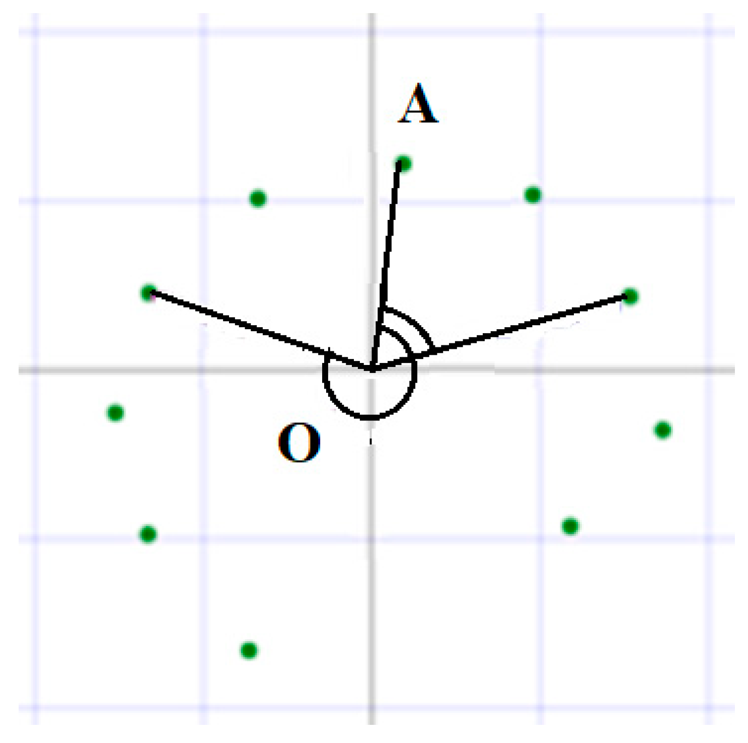
- Take a zero value (for example, radius OA vector = (0, 1) see Figure 3).
- (4)
- Find corners among the vectors from the center to each apex and OA (corners should be over the range of 0–360).
- (5)
- Sort corners from smaller to larger ones.
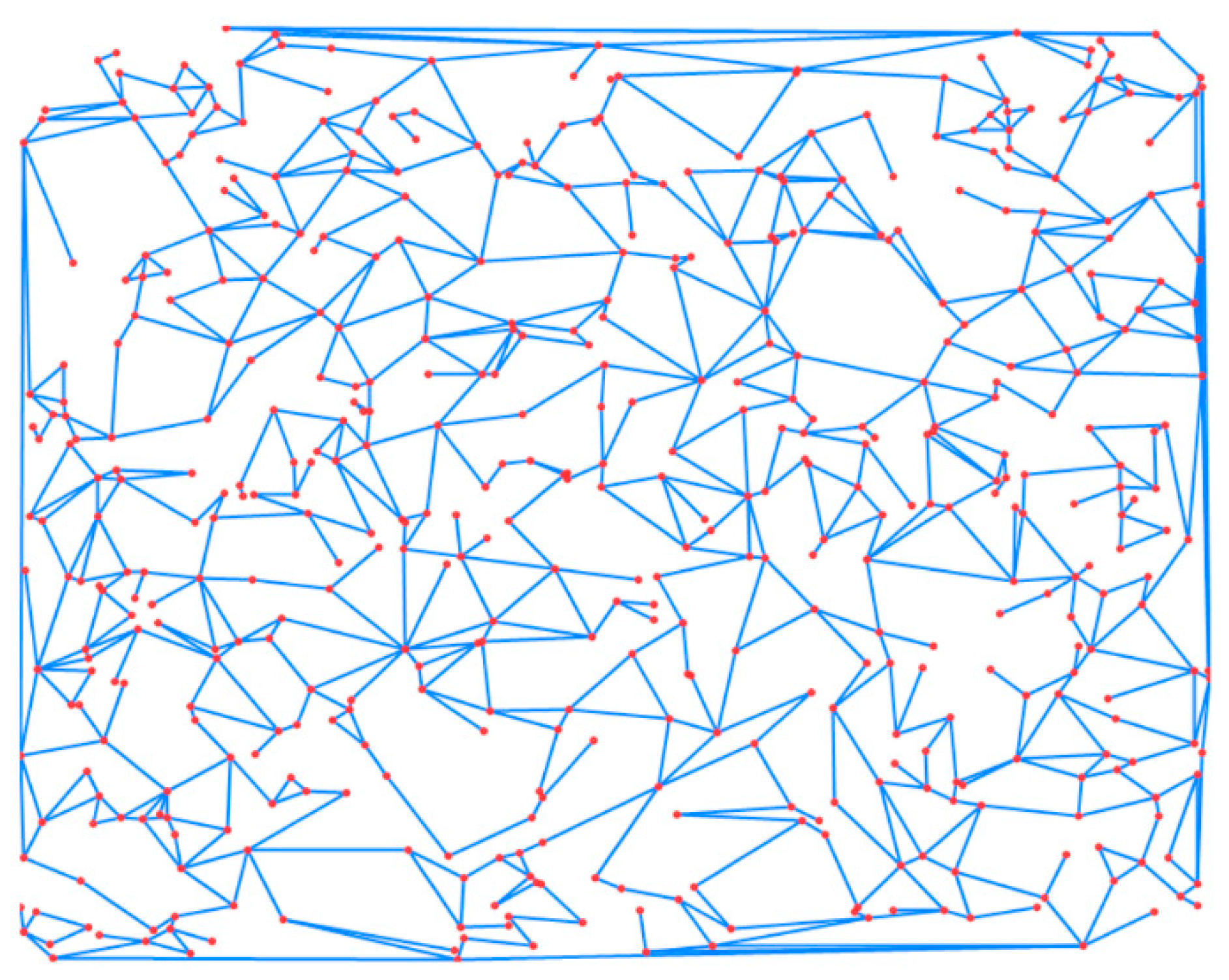
Using this algorithm, we can build different accidental planar networks; an example is presented in Figure 4.
4.2. Network Percolation Threshold Calculation Algorithm
The network percolation threshold algorithm used consists of the following steps [24]:
- (1)
- Randomly select two network junctions A and B, considering limits, with at least one intermediate junction between them.
- (2)
- Set the blocking probability value of the single junction (in the junction task) or link (for the link task) and randomly block the junction (or link) fraction which is equal to this probability.
- (3)
- Check for the presence of at least one “free” way in the network (a route which is included in the junction or link list) from junction A to junction B. If no “free” way is present (i.e., number of “free” ways is equal to 0), record 0. Otherwise, record 1.
- (4)
- Increase the blocking probability value of a single junction (for the junction task) or link (for the link task) on any value. Then, randomly block the fraction of network junctions (or links), equal to the specified probability value. Next, indicate the specific network junctions being excluded.
- (5)
- Repeat step 3, until all network junctions have been processed.
- (6)
- Return to step 2 and execute steps 3–5 times (for example, several hundred times). Repeat all steps (if the whole network is blocked) on all experiments. Indicate the number of embeddings, where at least one “free” way was indicated (designate as ). For example, at step h = 18 in 8, 12, 19, 56, 58, 76, 80, and 89 experiments with at least one “free” way, then (8 is the total number of “free” ways). Find the value , h—step number per step. Calculate the average cluster size of excluded junctions, the quantity of such clusters, etc. (on all N experiments per step). The average size of the cluster may be indicated as the ratio of all value sums obtained for this clustering step (on all Q experiments) to total number of experiments Q. For illustrative purposes, we can consider the following example: assume that, at step h = 6 in the first experiment, four clusters were obtained, each having a size of 15 junctions, whereas three clusters were obtained in the second experiment, two clusters were obtained in the third, etc. Then, the average number of clusters having a size 10 of blocked junctions would be equal to (4 + 3 + 2 +… + 5)/100.
- (7)
- Then, return to step 1 and repeat the implementation of steps 2–6, W times. For each W test, we can calculate the value . Index w indicates which W-test to study.
- (8)
- After completing the simulation, for each of the h steps, we can calculate the value , i.e., the average value of the probability ratio for passage through the network as a whole through unblocked junctions (or links for the task of link blocking) at each of the steps (considering different possible route configurations).
Calculating using this algorithm enables us to obtain a database for the dependency of the average ratio value of the probability of passage through the network as a whole on the fraction of blocked junctions (or links for link blocking tasks), at different average numbers of links, per junction (network density).
4.3. Calculating the Dependency of the Percolation Threshold Dependency on the Network Density (Average Number of Links per Crossroad)
The results of computational modeling and calculation of percolation threshold values for planar networks with an accidental number of links per junction for junction and link blocking tasks are presented in Table 1. Note that column 3 named “density” represents the average number of links per single junction, and the values of reverse link densities are specified in brackets. Column 4 named “threshold” represents the value of the percolation threshold (fraction of conductive junctions or links where network conductivity appears as a whole). The natural log values of percolation thresholds are specified in brackets.
Table 1 includes percolation threshold values as a fraction of conductive junctions (or links), where network conductivity appears. The fraction of blocked junctions (or links), where network conductivity disappears may be found as one minus the fraction of conductive junctions (or links).
Note that the percolation threshold values of planar networks with different densities for junction blocking tasks were calculated by the present authors in earlier works [25,26,27,28,29,30], where networks consisting of 100,000 junctions were used to carry out computational simulations. In order to undertake numerical experiments while solving network tasks, a network with 5000 junctions was used, requiring significant computational steps to successfully solve the tasks.
A 0.5 value of probability that the network transition is in a conducting state (see Figure 2) was selected as the percolation threshold of percolation network structures. However, note once again that we may take, for example, another value of transition probability of 0.95 or 0.99 (the percolation threshold would be set by the reliability criteria), i.e., we may calculate the fraction at which the total number of blocked junctions and/or links leads to the network losing the required level of efficiency.
It is important to note that the average number of links per single junction (network density) for a planar graph cannot exceed a value of 6. This is due to the Euler theorem [31], according to which, for a plane graph, the following equation should be fulfilled: V—E + F = 2, where V is the number of vertices in the graph, E is the number of edges, and F is the number of areas the graph separates in the plane.
In Figure 5, the dependencies of percolation threshold values of planar networks on the average number of network links per single junction (in junction blocking tasks [24] and in link blocking tasks) are presented.
To calculate the influence of the network’s structure density on the value of its percolation limits, it is necessary to analyze the data, shown in Table 1 and in Figure 5, and to calculate a functional dependency which may describe the influence of the network density on the value of its percolation limit. This enables us to calculate the link density of actual transport networks, to estimate the value of their percolation limit and, consequently, draw conclusions on the reliability of their structure, i.e., at which fraction of blocked junctions and/or links the network as a whole loses the required level of efficiency.
The results obtained can be used in the process of transport network construction or renovation in order to increase traffic potential and working capacity.
In [32,33,34] based on the topological structure of binding clusters proposed by Schklovskiy and de Zhen (“skeleton and dead ends”), the function of conditional flow probability (percolation) in grid Y(ξ, L) was obtained as follows:
where is the polynomial of degree i, ai represents its coefficients, is the fraction of blocked junctions, and ξc(L) is the fraction of blocked junctions, corresponding to the percolation threshold value which depends on the size of the network L. The polynomial S(ξ, L) of degree i may depend on the topological features of the network structure (network density, space symmetry, dimensionality etc.), which may be set during phenomenology with coefficients ai.
The main problem when describing percolation using Equation (1) is indicating the polynomial degree i and its coefficients. The shred use of Equation (1) and Hodge algebraic geometry methods [35], as well as Kadanoff–Wilson renormalization theory [36,37] with groups (see, e.g., [18]), enables us (in all cases) to calculate theoretical values of the percolation threshold for any regular structures [32,33,34]. In Hodge theory, algebraic varieties are studied (varieties, consisting of subsets, any of which comprise a set of solutions to any polynomial equations). Geometrical representations of algebraic varieties are called Hodge cycles. Linear combinations of such geometrical figures are called algebraic cycles [38].
The core of this approach is that we may depart from using Hodge methods and Kadanoff–Wilson renormalization groups to calculate the dependency of polynomial S(ξ, L) of degree i, from conditional probability Y(ξ, L) of the flow in the grid, as well as to calculate the influence of topological factors on such a dependency. Using Equation (1), we can derive the following:
where is the polynomial of degree i, ai designates its coefficients, ξ is the current value of the blocked junction fraction, and ξc(L) is the fraction of blocked junctions, which corresponds to the percolation threshold value (this depends on the size of network L). Considering that a value near to the percolation threshold is ξ ≈ ξc(L), then the polynomial value S(ξ, L) is small and may be expanded in series, restricted by two elements. After some manipulation, we can derive the following:
The righthand side of Equation (2) may be the function (or composed function) of certain variables, each of which is associated with any specific absolute concept of the network. For example, one of the variables may be the average number x of links (network density).
The described approach enables us to analyze the data specified in Table 1 and in Figure 5. It also enables us to present the dependency for the base logarithm of the percolation threshold lnP(x) on topological characteristics, for example, network density reciprocity (1/x), calculated as one divided by the average number of links per single network junction (see Figure 6). As may be inferred from Figure 6, the dependencies identified have a linear form and may be approximated by linear equations.
For planar structures in nodes tasks, the dependency of a percolation threshold log lnP(x) on the reciprocal of the network density (1/x) may be described using the following equation:
with a correlation number coefficient value and linear dependency equation equal to 0.99 (see righthand line 1 in Figure 6). In the links task, this equation becomes
with a correlation number coefficient value and linear dependency equation equal to 0.99 (see the righthand line 2 in Figure 6).
The focus here is a comparison of percolation features for accidental and regular planar networks. For example, the transport networks for New York or Mexico (see Figure 1) have a structure resembling a square lattice, while the transport networks of many other cities have structures which more closely resemble the structure shown in Figure 4. This leads us to question how the thresholds for such network blocking can differ at the same link density.
In Table 2, the percolation threshold values of some regular networks are shown (see Figure 7), and the cited literature is specified (where the source was not specified, the percolation threshold values were indicated in the numerical modeling results).
Figure 8 shows that dependencies of natural logs for percolation threshold values of regular networks from the reverse density of links are also described accurately using linear equations. For the nodes task, this equation becomes
with the value of the numeric correlation coefficient and linear dependence equation equal to 0.99 (see righthand line 1 in Figure 8). In the links task, this equation becomes
with the numeric correlation value and linear equations equal to 0.97 (see righthand line 2 in Figure 8).
Analysis of the results shows that the conductivity of any planar networks at identical densities of its bonds is larger than in the task of bond blocking compared with the task of node blocking. The percolation threshold (fraction of conductive nodes or bonds or where conductivity occurs) in the bond task is less than in the node task.
5. Discussion
Table 3 presents data on the density of transport bonds in any world cities, generated according to its graph analysis, as well as the value of blocking thresholds calculated using Equations (3) and (4). The values of network blocking values are specified in brackets, calculated from the analysis of real transport systems using numerical simulation. The blocking value is calculated using the following equation: one minus the percolation threshold calculated in Equation (3) or Equation (4). The values found in the analysis of the network graph are specified in brackets.
Table 4 presents data on the density of transport bonds in any world cities, calculated from graph analyses, as well as from the value of blocking thresholds calculated using Equations (5) and (6). The values of network blocking values are specified in brackets, calculated in the analysis of real transport systems using numerical simulation. The blocking value is calculated according to the following equation: one minus the percolation threshold calculated using Equation (5) or Equation (6).
A comparison of the data presented in Table 3 and Table 4 (which consider inaccuracies in reporting of traffic density and numerical simulation) enables us to draw two conclusions:
- 1.
- The transport networks of many cities in the world have structures which are close to an accidental structure and not regular planar networks.
- 2.
- An increase in network density leads to an increase in the blocking threshold of the network.
Today, rather often, overpasses and multilevel transport interchanges are constructed to increase traffic capacity. From a topological perspective, this changes its planarity. Earlier, in [25], the percolation features of nonplanar accidental networks were studied, and the following equation was found to calculate the conductivity threshold in node tasks:
where is the percolation threshold value, and x is the network density.
Taking the example of a network density equal to 2.65 (the mean density according to data from Table 3 and Table 4), for the percolation limit value of an accidental nonplanar network, we obtain 0.47. Thus, loss of conductivity for such structures occurs when the fraction of blocked nodes is greater than 0.53. Therefore, creating many nonplanar interchanges and overpasses in the transport network may significantly increase traffic capacity, but this is nevertheless associated with significant expenses due to the major construction work involved.
Let us consider the change in network topology due to the construction of multilevel interchanges and overpasses and their influence on the loss of efficiency in terms of bond blocking. Earlier, in [25], the percolation features of nonplanar accidental networks were studied, and the following equation was found for the conductivity limit in bond tasks:
where is the percolation threshold value, and x is the network density.
Taking a network density value equal to 2.65 as an example, we obtain 0.07 for the percolation limit value of the accidental nonplanar network. Thus, the loss of conductivity for such structures occurs when the fraction of blocked bonds is greater than 0.93. Accordingly, the creation of a large quantity of planar interchanges and overpasses in the transport network and in the event of bond blocking can also significantly increase its traffic capacity.
However, as mentioned earlier, this is due to the significant cost of capital construction of complex interchanges. When choosing specific urban planning solutions, it is necessary to consider that the percolation threshold of the transport network can be increased not only due to nonplanar overpasses, but also due to changes in density. In other words, you can add a small number of plank connections to the network graph instead of building tiered interchanges (if the cost of building them is higher).
6. Avenues for Future Research
In further investigations, the author plans to study the following issues:
- Table 3 includes data on the density of transport bonds in cities around the world and specific threshold values of blocking based on the analysis thereof, calculated using Equations (3) and (4). Note that the network blocking values were specified during an analysis of real transport systems using numerical simulation. The author further plans to study more city graphs, from which statistics can be gathered to study the correlation of blocking threshold values, calculated using Equations (3) and (4) and reported in the result of real traffic analysis. This will enable the development of an accurate percolation model.
- To estimate the reliability and efficiency of traffic, as well as the changes in traffic density throughout the day, it is necessary to indicate the average blocking probability of a network element at any given moment. Hence, different macroscopic traffic models will be studied in order to create an effective and accurate model of the influence of traffic characteristics and topology on the average probability of its elements blocking (drawing on the models proposed by Grinschields, Richards, Grindberg, El Hozaini, Underwood, Drake, and Pipes: the optimal speed, “Smart” driver, leader follow, cellular automata models, etc.). This will enable us to choose these characteristics as the core of the model and, consequently, to provide the required result after its modernization. Moreover, it will be useful to develop new models, for example, based on the description of stochastic systems including the possibility of self-organization and presence of memory of previous states.
7. Conclusions
Percolation theory methods may be used to investigate the operational reliability and ground transport network fault tolerance where any transport structure may be represented as a planar or almost planar graph with some nonlinear bonds (in real transport networks, this is associated with the presence of overpasses and multilevel interchanges).
In percolation theory, we may consider the solution to problems relating to the indication of blocked nodes and bond fractions for networks with different structures. In order to solve bond tasks, the fraction of nodes and bonds, which must be broken up to separate such a network into at least two isolated areas (or, conversely, the fraction of +–+ conductive bonds when conductivity occurs), is indicated. In the node task, the fraction of blocked nodes where network decomposition occurs to create isolated areas (or, vice versa, the fraction of conductive nodes when conductivity occurs) is indicated. The percolation threshold is the fraction of nonblocked nodes (for the node task) or unbroken bonds (for the bond task), where conductivity occurs between two randomly selected network nodes. For the same structure of percolation threshold values, node and bond tasks have different meanings. The value of the percolation threshold depends on the average number of bonds per single node of the network (density) and is the criterion of work reliability, i.e., it indicates at which fraction of blocked nodes and/or bonds the network loses the required level of efficiency as a whole.
The dependence of the blocking (percolation) threshold value on the network bond density can be mathematically expressed. This enables us to use the traffic map and indicates the average number of bonds per single node to then calculate the threshold value of when it blocks, which can be used when engineering and modernizing the road infrastructure. If such a blocking threshold is increased, we may calculate the necessary number of additional links.
Real transport networks have a topology which is closer to accidental networks than to regular ones. Given equal network density, an accidental planar network (if loss of efficiency is possible) is slightly inferior to regular structures.
Thus, if we know the total city road stretch and number of lanes, as well as daily vehicle dynamics, we may calculate the average traffic intensity on the basis of such data. Then, we can calculate the average probability that a network element will block at any given moment. This enables us to estimate the reliability and efficiency of the network, to analyze daily dynamics, and—if possible—to change the traffic structure accordingly.
Increasing transport bond density may increase the reliability and traffic capacity of the network. Moreover, in order to increase traffic capacity, we can choose to build overpasses and multilevel interchanges. From a topological perspective, this changes its planarity. In the case of the same link density with planar networks, random nonplanar networks have higher blocking threshold values. Creating a small number of nonplanar junctions and overpasses may significantly increase the traffic capacity of the network.
The results of this study can be methodically used as follows: the graph of the real transport network can be applied to investigate their percolation properties using previously described models and techniques. If we want to increase bandwidth and reliability (increase the percolation threshold), then various changes to the network graph may be proposed (either additional connections or tiered interchanges). Next, numerical simulations or calculations can be carried out using the percolation threshold equations obtained in the study for modified graphs (various proposed solutions). Then, the estimated option with the largest percolation threshold and minimal capital cost can be chosen in the implementation of city planning solutions. This solution will claim optimal reliability at minimal cost.
Funding
This research received no external funding.
Institutional Review Board Statement
Not applicable.
Informed Consent Statement
Not applicable.
Conflicts of Interest
The author declares no conflict of interest.
References
- Briani, M.; Cristiani, E. An easy-to-use algorithm for simulating traffic flow on networks: Theoretical study. Netw. Heterog. Media 2014, 9, 519–552. [Google Scholar] [CrossRef] [Green Version]
- Hui, M.; Bai, L.; Li, Y.; Wu, Q. Highway traffic flow nonlinear character analysis and prediction. Math. Probl. Eng. 2015, 20–27. [Google Scholar] [CrossRef] [Green Version]
- Ahn, G.-H.; Ki, Y.-K.; Kim, E.-J. Real-time estimation of travel speed using urban traffic information system and filtering algorithm. IET Intell. Transp. Syst. 2014, 8, 145–154. [Google Scholar] [CrossRef]
- Poole, A.; Kotsialos, A. Swarm intelligence algorithms for macroscopic traffic flow model validation with automatic assignment of fundamental diagrams. Appl. Soft Comput. 2016, 38, 134–150. [Google Scholar] [CrossRef] [Green Version]
- Guo, J.; Chen, F.; Xu, C. Traffic flow forecasting for road tunnel using PSO-GPR algorithm with combined kernel function. Math. Probl. Eng. 2017, 125–135. [Google Scholar] [CrossRef] [Green Version]
- Lesko, S.A.; Alyoshkin, A.S.; Barkov, A.A. Mathematical and software development of modeling and management of transport flows based on percolation stochastic model. CEUR Workshop Proc. 2017, 2064, 454–469. [Google Scholar]
- Lesko, S.A.; Alyoshkin, A.S.; Titov, V.V. Models and algorithms of optimization of routes in the transport network of the city. CEUR Workshop Proc. 2017, 2064, 438–453. [Google Scholar]
- Jiang, R.; Jin, C.; Zhang, H. Experimental and empirical investigations of traffic flow instability. Transp. Res. Procedia 2017, 23, 157–173. [Google Scholar] [CrossRef]
- Danchuk, V.; Bakulich, O.; Svatko, V. An Improvement in ant algorithm method for optimizing a transport route with regard to traffic flow. Procedia Eng. 2017, 425–434. [Google Scholar] [CrossRef]
- Pun-Cheng, L.S.; Chan, A.W. Optimal route computation for circular public transport routes with differential fare structure. Travel Behav. Soc. 2015, 3, 71–77. [Google Scholar] [CrossRef]
- Baranovskata, T.P.; Pavlov, D.A. Simulation of large-scale traffic networks using multiobjective optimization methods and considering structural dynamics. Political Netw. Electron. Sci. J. Kuban State Agrar. Univ. 2016, 120, 1686–1705. [Google Scholar]
- Pavlenko, P.F. Use of expert system and control module based on fuzzy logic in traffic adaptive management. Inst. Autom. Inf. Technol. NAN KR 2014, 2, 92–97. [Google Scholar]
- Trubicin, V.A.; Golub, D.I. Traffic management based on traffic and road capacity ratio. Bull. North-Cauc. Fed. Univ. 2013, 2, 89–92. [Google Scholar]
- Vlasov, A.A.; Chushkina, Z.A. Saturated Traffic Control Regional Architecture and Construction. Reg. Archit. Eng. 2014, 4, 152–156. [Google Scholar]
- Ziryanov, V.V. Peculiarities of main traffic diagram use on network level. Energy Resour. Sav. Ind. Transp. 2013, 21, 71–74. [Google Scholar]
- Filippova, D.M.; Chernyago, A.B.; Slobodchikova, N.A. Traffic flow distribution organizing coordinated traffic management. Bull. Irkutsk State Univ. 2013, 9, 172–176. [Google Scholar]
- Kaligin, N.N.; Uvaysov, S.U.; Uvaysova, A.S.; Uvaysova, S.S. Infrastructural review of the distributed telecommunication system of road traffic and its protocols. Russ. Technol. J. 2019, 7, 87–95. (In Russian) [Google Scholar] [CrossRef]
- Grimmet, G. Percolation, 2nd ed.; Springer: Berlin, Germany, 1999. [Google Scholar]
- Sahimi, M. Applications of Percolation Theory; Tailor & Francis: London, UK, 1992. [Google Scholar]
- Stauffer, D.; Aharony, A. Introduction to Percolation Theory; Tailor & Francis: London, UK, 1992. [Google Scholar]
- Feder, J. Fractals; Plenum Pressl: New York, NY, USA; London, UK, 1998. [Google Scholar]
- Lesko, S.A.; Alyoshkin, A.S.; Filatov, V.V. Stochastic and Percolating Models of Blocking Computer Networks Dynamics during Distribution of Epidemics of Evolutionary Computer Viruses. Russ. Technol. J. 2019, 7, 7–27. [Google Scholar] [CrossRef] [Green Version]
- Li, D.; Fu, B.; Wang, Y.; Lu, G.; Yehiel Berezin, H.; Stanley, E.; Havlin, S. Percolation transition in dynamical traffic network with evolving critical bottlenecks. Proc. Natl. Acad. Sci. USA 2015, 112, 669–672. [Google Scholar] [CrossRef] [Green Version]
- Zhukov, D.O.; Andrianova, E.G.; Lesko, S.A. The Influence of a Network’s Spatial Symmetry, Topological Dimension, and Density on its Percolation Threshold. Symmetry 2019, 11, 920. [Google Scholar] [CrossRef] [Green Version]
- Zhukov, D.; Khvatova, T.; Lesko, S.; Zaltsman, A. Managing social networks: Applying the Percolation theory methodology to understand individuals’ attitudes and moods. Technol. Forecast. Soc. Chang. 2017, 123, 234–245. [Google Scholar] [CrossRef]
- Zhukov, D.O.; Khvatova, T.Y.; Lesko, S.A.; Zaltsman, A.D. The influence of connection density on clusterization and percolation threshold during information distribution in social networks. Inform. Appl. 2018, 12, 90–97. [Google Scholar] [CrossRef]
- Khvatova, T.Y.; Zaltsman, A.D.; Zhukov, D.O. Information processes in social networks: Percolation and stochastic dynamics. CEUR Workshop Proc. 2017, 2064, 277–288. [Google Scholar]
- Lesko, S.; Aleshkin, A.; Zhukov, D. Reliability Analysis of the Air Transportation Network when Blocking Nodes and/or Connections Based on the Methods of Percolation Theory. IOP Conf. Ser. Mater. Sci. Eng. 2020, 714, 012016. [Google Scholar] [CrossRef]
- Zhukov, D.O.; Zaltcman, A.G.; Khvatova, T.Y. Forecasting Changes in States in Social Networks and Sentiment Security Using the Principles of Percolation Theory and Stochastic Dynamics. In Proceedings of the 2019 IEEE International Conference Quality Management, Transport and Information Security, Information Technologies IT and QM and IS 2019, Sochy, Russia, 23–27 September 2019; pp. 149–153. [Google Scholar] [CrossRef]
- Lesko, S.A.; Zhukov, D.O. Percolation models of information dissemination in social networks. In Proceedings of the 2015 IEEE International Conference on Smart City/SocialCom/SustainCom (SmartCity), Chengdu, China, 19–21 December 2015; pp. 213–216. [Google Scholar] [CrossRef]
- Trudeau, R.J. Introduction to Graph Theory; Corrected, Enlarged Republication, Edition; Dover Pub.: New York, NY, USA, 1993; p. 64. [Google Scholar]
- Gallyamov, S.R. A passing threshold of a simple cubic lattice in the site problem of Bethe lattice model. Vestn. Udmurt. Univ. Mat. Mekhanika Komp’yuternye Nauki 2008, 3, 109–115. (In Russian) [Google Scholar] [CrossRef] [Green Version]
- Gallyamov, S.R.; Mel’chukov, S.A. On one method of calculating percolation thresholds for square and diamond lattices in the percolation problem of knots. Vestn. Udmurt. Univ. Mat. Mekhanika Komp’yuternye Nauki 2009, 4, 33–44. (In Russian) [Google Scholar] [CrossRef] [Green Version]
- Gallyamov, S.R.; Mel’chukov, S.A. Hodge’s idea in percolation percolation threshold estimation by the unit cell. Vestn. Udmurt. Univ. Mat. Mekhanika Komp’yuternye Nauki 2011, 60–79. (In Russian) [Google Scholar] [CrossRef]
- Hodge, W.V.D. The Theory and Applications of Harmonic Integrals; Cambridge Mathematical Library: Cambridge, UK, 1952. [Google Scholar]
- Kadanoff, L.P.; Jotze, W.; Hamblen, D.; Hecht, R.; Lewis, E.A.S.; Palciauskas, V.V.; Rayl, M.; Swift, J.; Aspres, D.; Kane, J. Static Phenomena Near Critical Points: Theory and Experiment. Rev. Mod. Phys. 1967, 39, 395–431. [Google Scholar] [CrossRef]
- Wilson, K.G. Renormalization group and critical phenomena. Phys. Rev. B 1971, 4, 3174–3183. [Google Scholar] [CrossRef] [Green Version]
- Krasnov, V.A. Algebraic cycles on a real algebraic GM-manifold and their applications. Russ. Acad. Sci. Izv. Math. 1994, 43, 141–160. [Google Scholar] [CrossRef]
- Romeo, F.; Campolo, C.; Molinaro, A.; Berthet, A.O. DENM repetitions to enhance reliability of the autonomous mode in NR V2X sidelink. In Proceedings of the 2020 IEEE 91st Vehicular Technology Conference (VTC2020-Spring), Antwerp, Begium, 25–28 May 2020; pp. 1–5. [Google Scholar] [CrossRef]
- Qi, W.; Landfeldt, B.; Song, Q.; Guo, L.; Jamalipour, A. Traffic differentiated clustering routing in DSRC and C-V2X hybrid vehicular networks. IEEE Trans. Veh. Technol. 2020, 69, 7723–7734. [Google Scholar] [CrossRef] [Green Version]
- Zadobrischi, E.; Dimian, M. Vehicular Communications Utility in Road Safety Applications: A Step toward Self-Aware Intelligent Traffic Systems. Symmetry 2021, 13, 438. [Google Scholar] [CrossRef]
- Ahmed, S.H.; Bouk, S.H.; Yaqub, M.A.; Kim, D.; Song, H.; Lloret, J. CODIE: COntrolled Data and Interest Evaluation in vehicular named data networks. IEEE Trans. Veh. Technol. 2016, 65, 3954–3963. [Google Scholar] [CrossRef]
- Carli, R.; Dotoli, M.; Epicoco, N. Monitoring Traffic Congestion in Urban Areas through Probe Vehicles: A Case Study Analysis. Internet Technol. Lett. 2017, 1, e5. [Google Scholar] [CrossRef] [Green Version]
- Wang, S.; Zhang, X.; Cao, J.; He, L.; Stenneth, L.; Yu, P.S.; Li, Z.; Huang, Z. Computing urban traffic congestions by incorporating sparse GPS probe data and social media data. ACM Trans. Inf. Syst. 2017, 35, 30. [Google Scholar] [CrossRef]
Figure 1.
Traffic maps of several world conurbations (a—New York, b—Tokyo, c—Moscow, d—Mexico).

Figure 2.
The probability of percolation occurrence depending on the value of the fraction of conductive junctions (or links).
Figure 2.
The probability of percolation occurrence depending on the value of the fraction of conductive junctions (or links).

Figure 3.
Selection of points while sorting.

Figure 4.
Example of an accidental planar network consisting of 500 junctions with an average number of links equal to 2.9.
Figure 4.
Example of an accidental planar network consisting of 500 junctions with an average number of links equal to 2.9.

Figure 5.
Dependency of values percolation threshold values of planar accidental networks on network density (curve 1—junction task, curve 2—link task).
Figure 5.
Dependency of values percolation threshold values of planar accidental networks on network density (curve 1—junction task, curve 2—link task).

Figure 6.
Dependency of natural log percolation threshold value (lnP(x)) on accidental planar structures from the reciprocal of density (1/x).
Figure 6.
Dependency of natural log percolation threshold value (lnP(x)) on accidental planar structures from the reciprocal of density (1/x).

Figure 7.
Geometrical representation of some regular network structures (a–g).

Figure 8.
Dependency of natural log percolation threshold value (lnP(x)) on planar accidental structures from the reciprocal of density (1/x).
Figure 8.
Dependency of natural log percolation threshold value (lnP(x)) on planar accidental structures from the reciprocal of density (1/x).


Table 1.
Values of percolation thresholds for planar networks with an accidental structure.
| No. | Task Type | Density | Threshold |
|---|---|---|---|
| 1. | Junction blocking task [19,20,21] | 5.99 (0.167) | 0.500 (−0.693) |
| 2. | 5.40 (0.185) | 0.533 (−0.629) | |
| 3. | 4.80 (0.208) | 0.570 (−0.562) | |
| 4. | 4.50 (0.222) | 0.593 (−0.523) | |
| 5. | 4.20 (0.238) | 0.618 (−0.481) | |
| 6. | 3.90 (0.256) | 0.650 (−0.431) | |
| 7. | 3.60 (0.278) | 0.683 (−0.381) | |
| 8. | 3.42 (0.292) | 0.708 (−0.345) | |
| 9. | 3.18 (0.314) | 0.750 (−0.288) | |
| 10. | 2.94 (0.340) | 0.793 (−0.232) | |
| 11. | 2.70 (0.370) | 0.852 (−0.160) | |
| 12. | 2.46 (0.407) | 0.925 (−0.078) | |
| 13. | Link blocking task | 5.99 (0.167) | 0.395 (−0.929) |
| 14. | 5.69 (0.176) | 0.405 (−0.904) | |
| 15. | 5.39 (0.186) | 0.435 (−0.832) | |
| 16. | 5.09 (0.196) | 0.445 (−0.810) | |
| 17. | 4.49 (0.223) | 0.480 (−0.734) | |
| 18. | 4.19 (0.239) | 0.510 (−0.673) | |
| 19. | 3.89 (0.257) | 0.550 (−0.598) | |
| 20. | 3.59 (0.279) | 0.570 (−0.562) | |
| 21. | 3.29 (0.304) | 0.625 (−0.470) | |
| 22. | 2.99 (0.334) | 0.685 (−0.378) | |
| 23. | 2.87 (0.348) | 0.715 (−0.335) | |
| 24. | 2.70 (0.370) | 0.770 (−0.261) | |
| 25. | 2.58 (0.388) | 0.805 (−0.217) | |
| 26. | 2.39 (0.418) | 0.900 (−0.105) |
Table 2.
Percolation threshold values for planar networks with regular structures.
| No. | Task Type | Density | Threshold |
|---|---|---|---|
| 1. | Node blocking task | 2.7 (0.37)–f in Figure 5. | 0.74 (−0.30) |
| 2. | 3 (0.33)–d in Figure 5 [17]. | 0.70 (−0.36) | |
| 3. | 3.40 (0.29)–g in Figure 5. | 0.64 (−0.45) | |
| 4. | 4 (0.25)–a in Figure 5 [17]. | 0.59 (−0.53) | |
| 5. | 4.5 (0.22)–e in Figure 5. | 0.56 (−0.58) | |
| 6. | 6 (0.17)–b in Figure 5. | 0.50 (−0.69) | |
| 7. | 6 (0.17)–c in Figure 5 [17]. | 0.50 (−0.69) | |
| 8. | Bond blocking tasks | 2.7 (0.37)–f in Figure 5. | 0.69 (−0.37) |
| 9. | 3 (0.33)–d in Figure 5 [17]. | 0.65 (−0.43) | |
| 10. | 3.40 (0.29)–g in Figure 5. | 0.52 (−0.65) | |
| 11. | 4 (0.25)–a in Figure 5 [17]. | 0.50 (−0.69) | |
| 12. | 6 (0.17)–b in Figure 5. | 0.36 (−1.02) | |
| 13. | 6 (0.17)–c in Figure 5 [17]. | 0.35 (−1.05) |
Table 3.
Densities of transport bonds in any world cities and values of their blocking thresholds identified using models of accidental networks.
Table 3.
Densities of transport bonds in any world cities and values of their blocking thresholds identified using models of accidental networks.
| No. | City | Density | Blocking Threshold in Node Tasks according to Equation (3) | Blocking Threshold in Link Tasks according to Equation (4) |
|---|---|---|---|---|
| 1. | New York | 2.85 | 0.18 (0.19) | 0.27 (0.21) |
| 2. | Istanbul | 2.91 | 0.19 (0.19) | 0.29 (0.21) |
| 3. | Madrid | 2.77 | 0.16 (0.18) | 0.25 (0.21) |
| 4. | Beijing | 2.70 | 0.14 (0.17) | 0.23 (0.27) |
| 5. | Paris | 2.63 | 0.11 (0.16) | 0.20 (0.19) |
| 6. | Moscow | 2.51 | 0.08 (0.13) | 0.16 (0.17) |
| 7. | London | 2.39 | 0.03 (0.11) | 0.10 (0.14) |
Table 4.
Densities of transport bonds in any world cities and the values of their blocking thresholds calculated using models of regular networks.
Table 4.
Densities of transport bonds in any world cities and the values of their blocking thresholds calculated using models of regular networks.
| No. | City | Density | Blocking Threshold in Node Tasks according to Equation (5) | Blocking Threshold in Link Tasks according to Equation (6) |
|---|---|---|---|---|
| 1. | New York | 2.85 | 0.28 (0.19) | 0.33 (0.21) |
| 2. | Istanbul | 2.91 | 0.29 (0.19) | 0.35 (0.21) |
| 3. | Madrid | 2.77 | 0.26 (0.18) | 0.31 (0.21) |
| 4. | Beijing | 2.70 | 0.25 (0.17) | 0.29 (0.27) |
| 5. | Paris | 2.63 | 0.23 (0.16) | 0.27 (0.19) |
| 6. | Moscow | 2.51 | 0.21 (0.13) | 0.22 (0.17) |
| 7. | London | 2.39 | 0.17 (0.11) | 0.17 (0.14) |
Publisher’s Note: MDPI stays neutral with regard to jurisdictional claims in published maps and institutional affiliations. |
© 2021 by the author. Licensee MDPI, Basel, Switzerland. This article is an open access article distributed under the terms and conditions of the Creative Commons Attribution (CC BY) license (https://creativecommons.org/licenses/by/4.0/).
Share and Cite
MDPI and ACS Style
Aleshkin, A. The Influence of Transport Link Density on Conductivity If Junctions and/or Links Are Blocked. Mathematics 2021, 9, 1278. https://doi.org/10.3390/math9111278
AMA Style
Aleshkin A. The Influence of Transport Link Density on Conductivity If Junctions and/or Links Are Blocked. Mathematics. 2021; 9(11):1278. https://doi.org/10.3390/math9111278
Chicago/Turabian StyleAleshkin, Anton. 2021. "The Influence of Transport Link Density on Conductivity If Junctions and/or Links Are Blocked" Mathematics 9, no. 11: 1278. https://doi.org/10.3390/math9111278
Note that from the first issue of 2016, this journal uses article numbers instead of page numbers. See further details here.