
Fire Risk Sub-Module Assessment under Solvency II. Calculating the Highest Risk Exposure


Abstract
:
1. Introduction
2. Solvency II
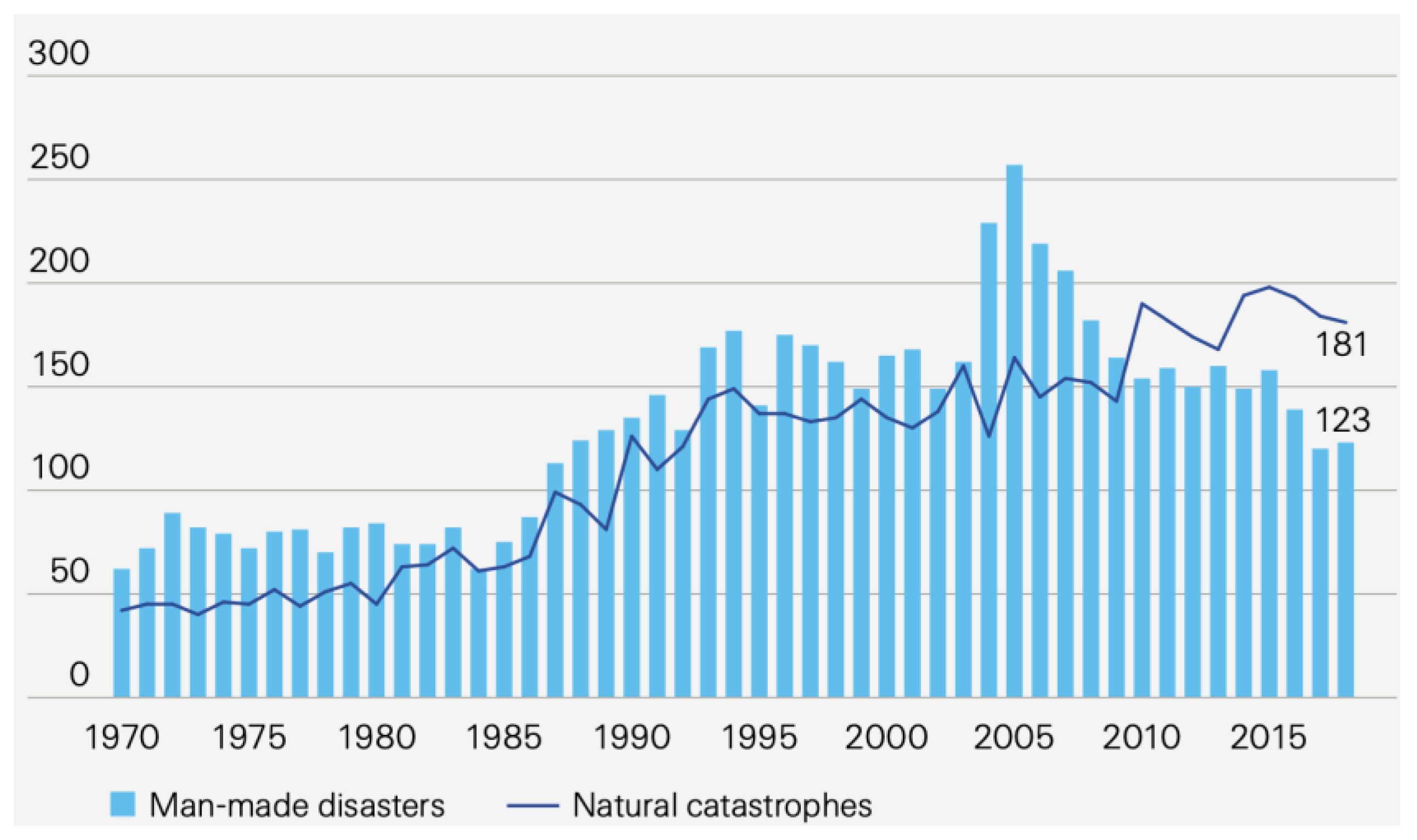
2.1. Man-Made Catastrophe Risk
Fire Risk Sub-Module
3. Determination of the Highest Concentration of Risk for an Insurance Company
3.1. Methodology
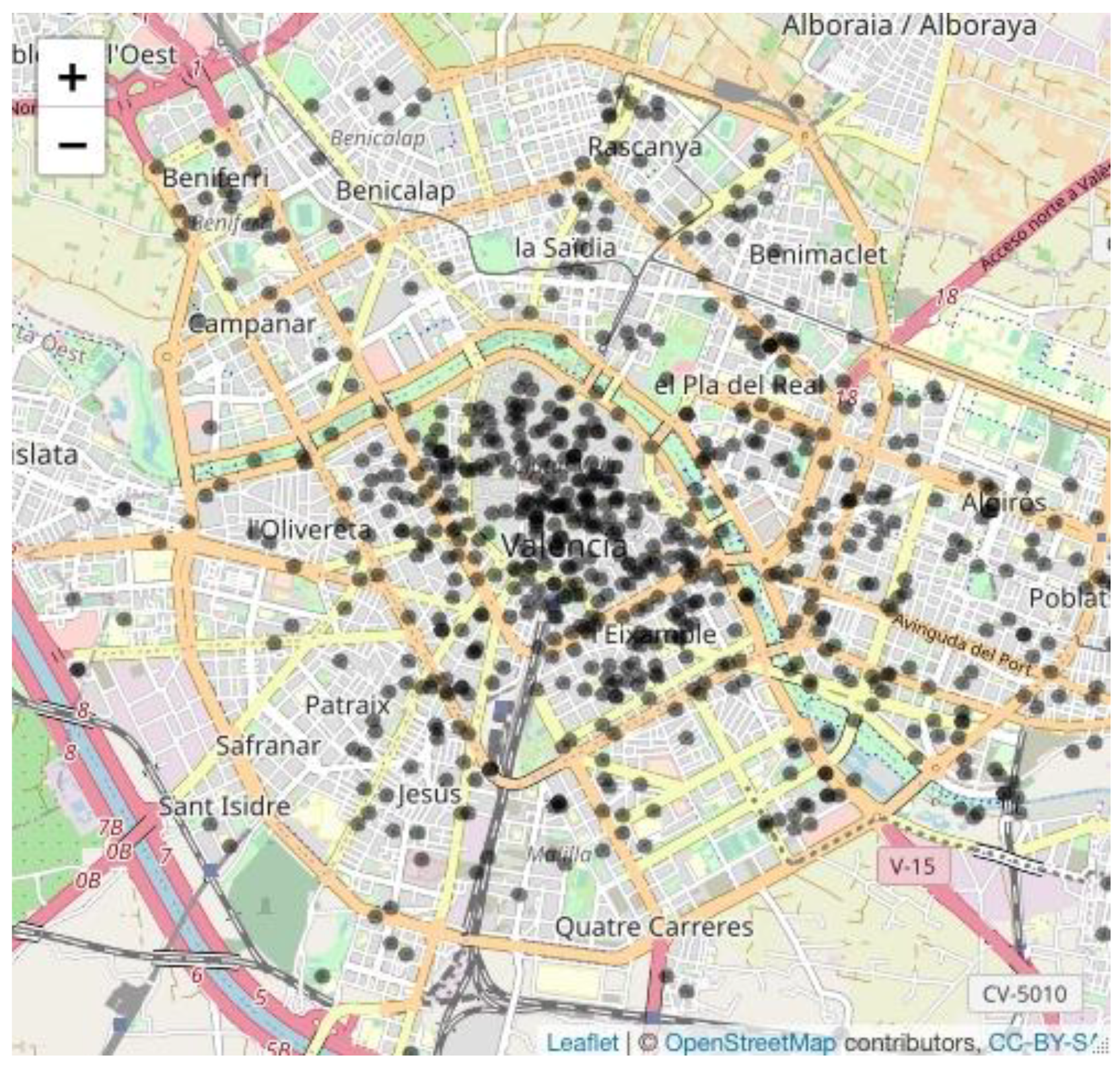
3.2. Dataset
4. Case Study Results and Discussion
- data: original dataframe to which a first column (ref) was added to list the policyholders consecutively.
- distance.matrix: matrix with the selected distance (Haversine by default) for each pair of geographic points.
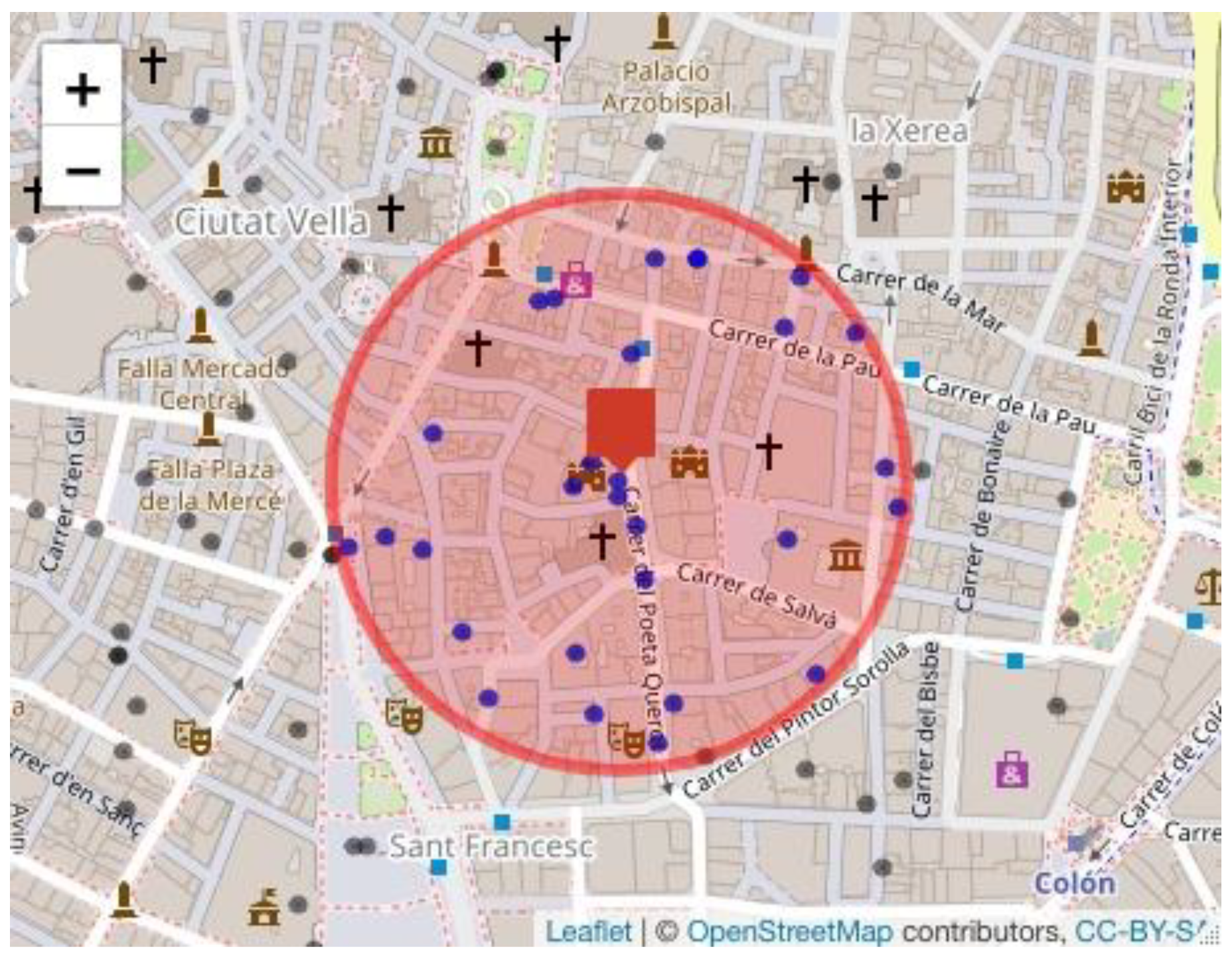
- cumulus.matrix: risk matrix, in which each policyholder constitutes the centroid of a risk cluster.
- maximum.cumulus: amount of the highest risk for the insurance company.
- identification.cumulus: policyholder representing the centroid of the highest risk cluster.
- cumulus.data: dataframe made up of the policyholders who form the highest risk cluster.
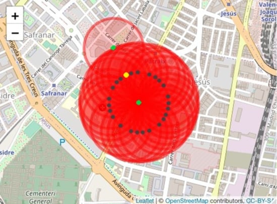
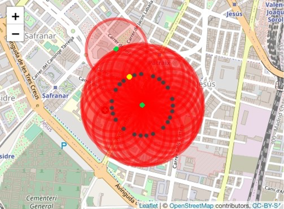
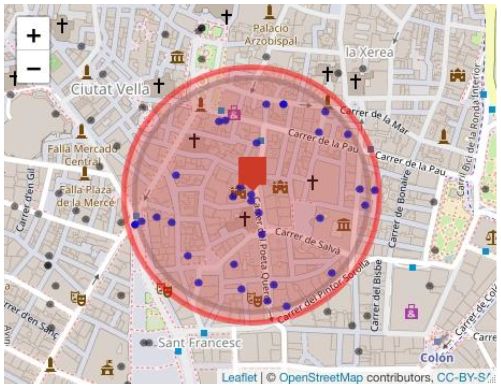
- Scenario 1. Maintain policyholder 2266 as the centroid of the highest risk cluster and extend the cluster radius by 20 m to identify the policyholders who are within the extended radius. The results of this scenario 1 using the Haversine distance are obtained by executing the following instruction:
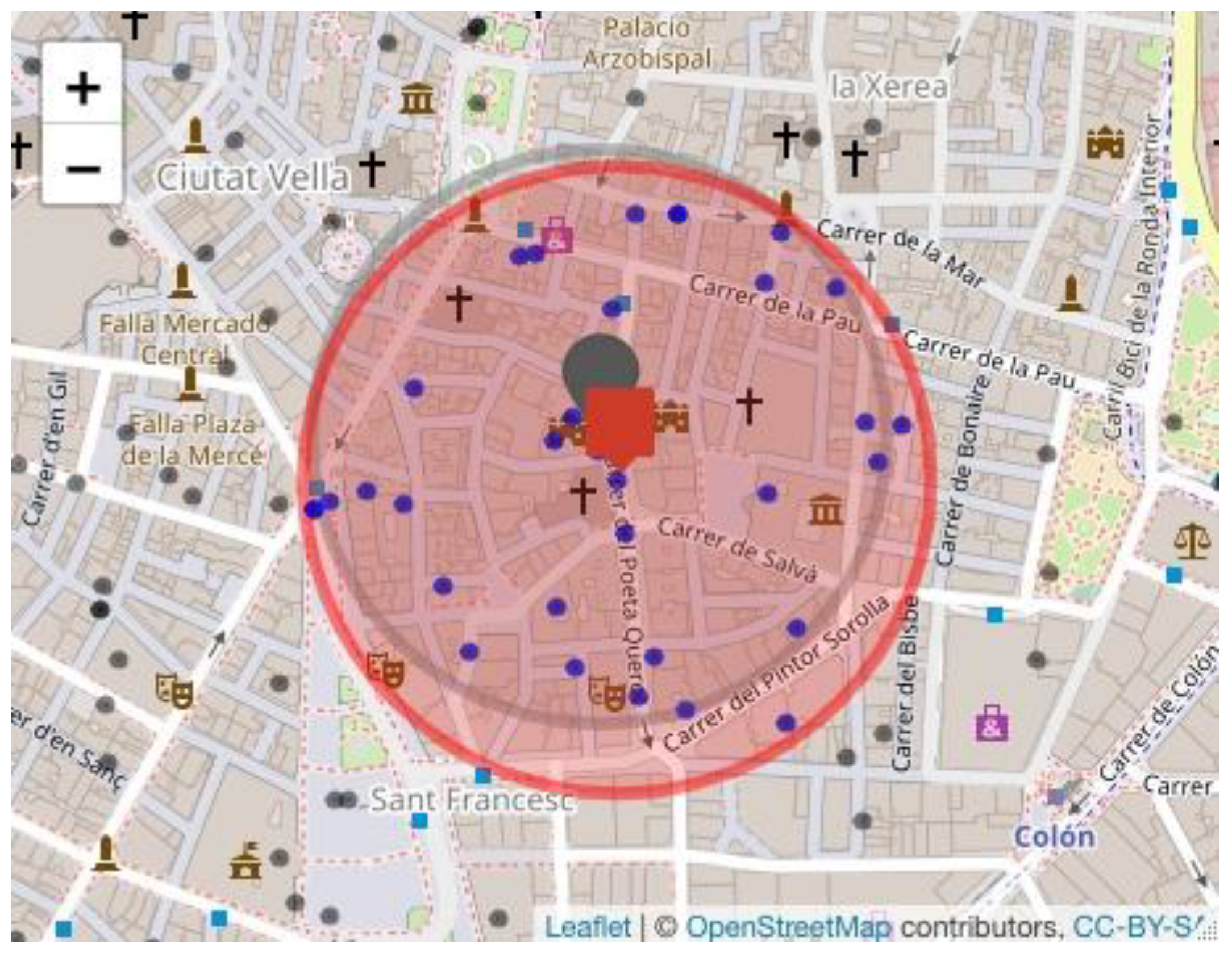
- Scenario 2. Determine a new risk cluster considering all the policyholders who are located in the new radius (200 m plus the margin of error). To obtain the results of this scenario, we execute the following instruction:result3 ← cumulus(data, margin = 20, extended = 2).
5. Conclusions
Supplementary Materials
Author Contributions
Funding
Institutional Review Board Statement
Informed Consent Statement
Data Availability Statement
Conflicts of Interest
Appendix A
Appendix B
Appendix C
References
- European Parliament of the Council. Directive 2009/138/EC of the European Parliament and of the Council of 25 November 2009 on the Taking-Up and Pursuit of the Business of Insurance and Reinsurance (Solvency II). 2009. Available online: https://eur-lex.europa.eu/legal-content/en/TXT/?uri=CELEX:32009L0138 (accessed on 1 June 2021).
- European Parliament of the Council. Commission Delegated Regulation (EU) 2015/35 of 10 October 2014 Supplementing Directive 2009/138/EC of the European Parliament and of the Council on the Taking-Up and Pursuit of the Business of Insurance and Reinsurance (Solvency II). 2015. Available online: https://eur-lex.europa.eu/eli/reg_del/2015/35/oj (accessed on 1 June 2021).
- SWISS RE. Sigma Nº2/2019: Natural Catastrophes and Man-Made Disasters in 2018: “Secondary” Perils on the Frontline. 2019. Available online: https://www.swissre.com/dam/jcr:c37eb0e4-c0b9-4a9f-9954-3d0bb4339bfd/sigma2_2019_en.pdf (accessed on 1 June 2021).
- European Parliament of the Council. Commission Delegated Regulation (EU) 2019/981 of 8 March 2019 Amending Delegated Regulation (EU) 2015/35 Supplementing Directive 2009/138/EC on the Taking-Up and Pursuit of the Business of Insurance and Reinsurance (Solvency II). 2019. Available online: https://eur-lex.europa.eu/legal-content/EN/TXT/?uri=CELEX%3A32019R0981 (accessed on 1 June 2021).
- Yeo, A.C.; Smith, K.A.; Willis, R.J.; Brooks, M. Clustering technique for risk classification and prediction of claim costs in the automobile insurance industry. Intell. Syst. Acc. Financ. Manag. 2011, 10, 39–50. [Google Scholar] [CrossRef]
- Abolmakarem, S.; Abdi, F.; Khalili-Damghani, K. Insurance customer segmentation using clustering approach. Int. J. Knowl. Eng. Data Min. 2016, 4, 18–39. [Google Scholar] [CrossRef]
- Zhuang, K.; Wu, S.; Gao, X. Auto Insurance Business Analytics Approach for Customer Segmentation Using Multiple Mixed-Type Data Clustering Algorithms. Teh. Vjesn. 2011, 25, 1783–1791. [Google Scholar]
- Hidalgo, H.; Chipulu, M.; Ojiako, U. Risk segmentation in Chilean social health insurance. Int. J. Health Care Qual. Assur. 2013, 26, 666–681. [Google Scholar] [CrossRef] [PubMed]
- Alkan, H.; Celebi, H. The Implementation of Positioning System with Trilateration of Haversine Distance. In Proceedings of the 30th Annual International Symposium on Personal, Indoor and Mobile Radio Communications (PIMRC), Istanbul, Turkey, 8–11 September 2019; pp. 1–6. Available online: https://ieeexplore.ieee.org/abstract/document/8904289 (accessed on 1 June 2021).
- Alam, C.N.; Manaf, K.; Atmadja, A.R.; Aurum, D.K. Implementation of Haversine Formula for Counting Event Visitor in the Radius Based on Android Application. In Proceedings of the 2016 4th International Conference on Cyber and IT Service Management IEEE, Bandung, Indonesia, 26–27 April 2016; pp. 1–6. [Google Scholar]
- Basyir, M.; Nasir, M.; Suryati, S.; Mellyssa, W. Determination of nearest emergency service office using haversine formula based on android platform. Emit. Int. J. Eng. Technol. 2017, 5, 270–278. [Google Scholar] [CrossRef]
- Cho, J.H.; Baik, E.Y. Geo-spatial Analysis of the Seoul Subway Station Areas Using the Haversine Distance and the Azimuth Angle Formulas. J. Inf. Technol. Serv. 2018, 12, 139–150. [Google Scholar]
- Dauni, P.; Firdaus, M.D.; Asfariani, R.; Saputra, M.I.N.; Hidayat, A.A.; Zulfikar, W.B. Implementation of Haversine Formula for School Location Tracking. J. Phys. Conf. Ser. 2017, 1402, 077028. [Google Scholar] [CrossRef]
- Hartanto, A.D.; Susanto, M.R.; Ilham, H.D.; Retnaningsih, R.; Nurdiyanto, H. Mobile Technologies of Formulation Haversine Application and Location Based Service. In Proceedings of the Joint Workshop KO2PI and the 1st International Conference on Advance & Scientific Innovation, Medan, Indonesia, 23–24 April 2018. [Google Scholar]
- Huang, J.; Huang, H. Looking around in the Neighbourhood: Location Estimation of Outdoor Urban Images. IET Image Process. 2021, 1–13. [Google Scholar] [CrossRef]
- Van Kampen, J.; Knapen, L.; Pauwels, E.; Van der Mei, R.; Dugundji, E.R. Bicycle Parking in Station Areas in the Netherlands. Procedia Comput. Sci. 2021, 184, 338–345. [Google Scholar] [CrossRef]
- Sinnott, R.W. Virtues of the Haversine. Sky Telesc. 1984, 68, 159. [Google Scholar]
- Vincenty, T. Direct and inverse solutions of geodesics on the ellipsoid with application of nested equations. Surv. Rev. 1975, 23, 88–93. Available online: https://www.ngs.noaa.gov/PUBS_LIB/inverse.pdf (accessed on 1 June 2021). [CrossRef]
- Hijmans, R.J. Geosphere: Spherical Trigonometry. R Package Version 1.5-10. 2019. Available online: https://CRAN.R-project.org/package=geosphere (accessed on 1 June 2021).
- Che, J.; Karambelkar, B.; Xie, Y. Leaflet: Create Interactive Web Maps with the JavaScript ’Leaflet’. R package version 2.0.3. 2019. Available online: https://CRAN.R-project.org/package=leaflet (accessed on 1 June 2021).


| Statistic | Sum Insured (€) |
|---|---|
| Minimum | 34,099.73 |
| First quartile | 194,856.66 |
| Median | 461,285.27 |
| Third quartile | 1,120,281.02 |
| Mean | 1,249,490.66 |
| Maximum | 12,388,953.79 |
| Standard deviation | 1,639,387.156 |
| Ref | id | Longitude | Latitude | Sum.Insured | Highest.Sum.Insured | Insured.Cluster |
|---|---|---|---|---|---|---|
| 231 | 2266 | −0.3745403 | 39.4724532 | 3,603,539 | 41,431,645 | 29 |
| 899 | 2940 | −0.3745509 | 39.4723678 | 1,467,116 | 41,242,621 | 29 |
| 405 | 667 | −0.3743963 | 39.4721817 | 295,888 | 40,118,952 | 27 |
| 929 | 1552 | −0.3748926 | 39.4713922 | 255,455 | 32,632,384 | 24 |
| 717 | 1394 | −0.3743319 | 39.4718396 | 1,979,428 | 32,484,721 | 22 |
| 510 | 1517 | −0.3751963 | 39.4735817 | 565,817 | 31,562,826 | 24 |
| 376 | 494 | −0.3747399 | 39.4709996 | 117,543 | 30,211,509 | 22 |
| 635 | 685 | −0.3748998 | 39.4724242 | 134,527 | 29,676,494 | 27 |
| 762 | 878 | −0.3731713 | 39.4720993 | 372,652 | 29,629,749 | 24 |
| 228 | 3067 | −0.3723715 | 39.4725479 | 3,608,698 | 28,545,751 | 17 |
| 72 | 3111 | −0.3747591 | 39.4725809 | 552,030 | 28,406,181 | 26 |
| 890 | 2927 | −0.3729262 | 39.4712578 | 9,610,409 | 27,250,428 | 20 |
| 213 | 1899 | −0.3744403 | 39.4732532 | 154,923 | 26,992,852 | 22 |
| 984 | 2453 | −0.3761294 | 39.472035 | 696,180 | 26,919,386 | 26 |
| 413 | 2998 | −0.3760352 | 39.4727656 | 442,312 | 26,690,708 | 26 |
| 752 | 642 | −0.3722713 | 39.4722993 | 130,279 | 26,005,069 | 17 |
| 365 | 524 | −0.3764342 | 39.4721113 | 6,467,363 | 26,004,924 | 26 |
| 334 | 2656 | −0.3739059 | 39.4738459 | 250,591 | 25,825,806 | 22 |
| 696 | 2640 | −0.3739059 | 39.4738459 | 4,211,254 | 25,825,806 | 22 |
| 2 | 2511 | −0.3767362 | 39.4720473 | 999,983 | 25,294,012 | 27 |
| 531 | 1831 | −0.3750513 | 39.4736109 | 1,980,909 | 25,095,463 | 23 |
| 101 | 480 | −0.3755984 | 39.4711045 | 104,032 | 23,984,461 | 25 |
| 855 | 2638 | −0.3731927 | 39.4734223 | 829,238 | 23,877,075 | 21 |
| 537 | 2725 | −0.3742187 | 39.4708188 | 1,265,507 | 23,729,718 | 19 |
| 120 | 2926 | −0.3740933 | 39.4710726 | 91,244 | 23,719,724 | 19 |
| 790 | 2910 | −0.373064 | 39.4737415 | 123,686 | 23,446,660 | 19 |
| 42 | 2985 | −0.3758014 | 39.4715086 | 246,718 | 22,861,348 | 24 |
| 179 | 712 | −0.3742403 | 39.4738532 | 191,377 | 22,659,420 | 22 |
| 641 | 1352 | −0.372606 | 39.4733964 | 682,947 | 19,410,813 | 16 |
| Ref | id | Longitude | Latitude | Sum.Insured | Highest.Sum.Insured | Insured.Cluster |
|---|---|---|---|---|---|---|
| 405 | 667 | −0.3743963 | 39.4721817 | 295,888 | 45,090,147 | 34 |
| 72 | 3111 | −0.3747591 | 39.4725809 | 552,030 | 44,710,177 | 34 |
| 231 | 2266 | −0.3745403 | 39.4724532 | 3,603,539 | 44,695,192 | 33 |
| 899 | 2940 | −0.3745509 | 39.4723678 | 1,467,116 | 44,695,192 | 33 |
| 635 | 685 | −0.3748998 | 39.4724242 | 134,527 | 44,214,279 | 33 |
| 717 | 1394 | −0.3743319 | 39.4718396 | 1,979,428 | 40,521,606 | 30 |
| 510 | 1517 | −0.3751963 | 39.4735817 | 565,817 | 37,391,765 | 29 |
| 213 | 1899 | −0.3744403 | 39.4732532 | 154,923 | 36,989,629 | 30 |
| 531 | 1831 | −0.3750513 | 39.4736109 | 1,980,909 | 34,662,865 | 27 |
| 762 | 878 | −0.3731713 | 39.4720993 | 372,652 | 34,480,801 | 28 |
| 376 | 494 | −0.3747399 | 39.4709996 | 117,543 | 33,791,787 | 26 |
| 228 | 3067 | −0.3723715 | 39.4725479 | 3,608,698 | 33,223,488 | 26 |
| 929 | 1552 | −0.3748926 | 39.4713922 | 255,455 | 33,064,176 | 27 |
| 413 | 2998 | −0.3760352 | 39.4727656 | 442,312 | 32,482,616 | 31 |
| 502 | 2593 | −0.3720783 | 39.472529 | 497,248 | 31,950,599 | 22 |
| 365 | 524 | −0.3764342 | 39.4721113 | 6,467,363 | 30,998,182 | 35 |
| 984 | 2453 | −0.3761294 | 39.472035 | 696,180 | 30,107,169 | 32 |
| 2 | 2511 | −0.3767362 | 39.4720473 | 999,983 | 29,944,752 | 35 |
| 179 | 712 | −0.3742403 | 39.4738532 | 191,377 | 29,548,613 | 27 |
| 39 | 2538 | −0.376853 | 39.472 | 110,133 | 29,378,935 | 34 |
| 795 | 2551 | −0.376853 | 39.472 | 2,162,243 | 29,378,935 | 34 |
| 752 | 642 | −0.3722713 | 39.4722993 | 130,279 | 28,919,798 | 22 |
| 890 | 2927 | −0.3729262 | 39.4712578 | 9,610,409 | 28,467,010 | 23 |
| 101 | 480 | −0.3755984 | 39.4711045 | 104,032 | 27,151,364 | 27 |
| 334 | 2656 | −0.3739059 | 39.4738459 | 250,591 | 27,138,018 | 25 |
| 696 | 2640 | −0.3739059 | 39.4738459 | 4,211,254 | 27,138,018 | 25 |
| 855 | 2638 | −0.3731927 | 39.4734223 | 829,238 | 25,856,503 | 22 |
| 537 | 2725 | −0.3742187 | 39.4708188 | 1,265,507 | 25,856,380 | 23 |
| 42 | 2985 | −0.3758014 | 39.4715086 | 246,718 | 25,804,871 | 26 |
| 120 | 2926 | −0.3740933 | 39.4710726 | 91,244 | 25,108,207 | 22 |
| 242 | 1690 | −0.3738458 | 39.4707353 | 493,923 | 24,698,915 | 21 |
| 790 | 2910 | −0.373064 | 39.4737415 | 123,686 | 23,877,075 | 21 |
| 641 | 1352 | −0.372606 | 39.4733964 | 682,947 | 23,706,756 | 20 |
| 108 | 1075 | −0.3730155 | 39.4706526 | 394,955 | 21,838,165 | 18 |
Publisher’s Note: MDPI stays neutral with regard to jurisdictional claims in published maps and institutional affiliations. |
© 2021 by the authors. Licensee MDPI, Basel, Switzerland. This article is an open access article distributed under the terms and conditions of the Creative Commons Attribution (CC BY) license (https://creativecommons.org/licenses/by/4.0/).
Share and Cite
Badal-Valero, E.; Coll-Serrano, V.; Segura-Gisbert, J. Fire Risk Sub-Module Assessment under Solvency II. Calculating the Highest Risk Exposure. Mathematics 2021, 9, 1279. https://doi.org/10.3390/math9111279
Badal-Valero E, Coll-Serrano V, Segura-Gisbert J. Fire Risk Sub-Module Assessment under Solvency II. Calculating the Highest Risk Exposure. Mathematics. 2021; 9(11):1279. https://doi.org/10.3390/math9111279
Chicago/Turabian StyleBadal-Valero, Elena, Vicente Coll-Serrano, and Jorge Segura-Gisbert. 2021. "Fire Risk Sub-Module Assessment under Solvency II. Calculating the Highest Risk Exposure" Mathematics 9, no. 11: 1279. https://doi.org/10.3390/math9111279