Not Another Computer Algebra System: Highlighting wxMaxima in Calculus

Abstract

This article introduces and explains a computer algebra system (CAS) wxMaxima for Calculus teaching and learning at the tertiary level. The didactic reasoning behind this approach is the need to implement an element of technology into classrooms to enhance students’ understanding of Calculus concepts. For many mathematics educators who have been using CAS, this material is of great interest, particularly for secondary teachers and university instructors who plan to introduce an alternative CAS into their classrooms. By highlighting both the strengths and limitations of the software, we hope that it will stimulate further debate not only among mathematics educators and software users but also also among symbolic computation and software developers.

1. Introduction

A computer algebra system (CAS) is a program that can solve mathematical problems by rearranging formulas and finding a formula that solves the problem, as opposed to just outputting the numerical value of the result. Maxima is a full-featured open-source CAS: the software can serve as a calculator, provide analytical expressions, and perform symbolic manipulations. Furthermore, it offers a range of numerical analysis methods for equations or systems of equations that otherwise cannot be solved analytically. It can sketch graphical objects with excellent quality.

What is wxMaxima, then? wxMaxima is a document-based graphical user interface (GUI) for the CAS Maxima. It allows us for using all of Maxima’s functions. Additionally, it provides convenient wizards for accessing the most commonly used features, including inline plots and simple animations. Similar to Maxima, wxMaxima is free of charge, and it is released and distributed under the terms of the GNU General Public License (GPL). This allows for everyone to modify and distribute it, as long as its license remains unmodified. In this article, we use the term “wxMaxima” more often, but the terms “Maxima” and “wxMaxima” can be used interchangeably.

Maxima is different from other well-known so-called 3M mathematical software (Maple, Matlab, Mathematica), as they are commercial and one needs to purchase a license before using them. Other open-source mathematics software include Axiom, Reduce, SageMath, Octave and Scilab (both are for numerical computation), R (for statistical computing), and GeoGebra (for interactive geometry and algebra), where the latter is quite well-known globally among mathematics educators.

Apart from being free and easy to install, Maxima is also updated continuously. Currently, Maxima can run natively without emulation on the following operating systems: Windows, Mac OS X, Linux, Berkeley Software Distribution (FreeBSD), Solaris, and Android. An executable file can be downloaded from Maxima’s website [1]. In particular, the installation file for Windows operating system is available for download at an open-source software community resource SourceForge [2]. One can simply double-click the executable file and follow the instruction accordingly. After the installation is completed, the software is ready to be launched. The whole process takes less than three minutes in total, depending on the Internet connection speed.

This software is introduced because it is free and under the GPL. As a comparison, the total combined cost for purchasing 3M software is almost USD 5500 for an educational license (see

Table 1. Software packages and the individuals or institutions through which they were first developed, the year they were launched, and estimated cost in USD.

Software	Creator	Launched	Cost (USD)
Axiom	Richard Jenks	1977	Free
Magma	University of Sydney	1990	USD 1140
Maple	University of Waterloo	1980	USD 2390
Mathematica	Wolfram Research	1986	USD 2495
Maxima	Bill Schelter et al.	1976	Free
Matlab	MathWorks	1989	USD 3150
SageMath	William A. Stein	2005	Free

). Although the expenditure for personal and student licenses are much lower than those for commercial and professional licenses, for colleagues and practitioners in many developing countries, the price is still considered to be costly. Having this in mind, we promote an open-source software that benefits many people who have limited resources, particularly in less affluent countries.

For teaching and learning mathematics, Maxima is fairly accessible by many people. Although SageMath is popular among university professors for teaching Calculus and Linear Algebra thanks to its user-friendly cloud, the server is rather slow, particularly if one attempts to access it from a developing country with modest Internet connectivity. SageMath can be downloaded and installed locally, but it is a huge file. Thus, it is another hindrance for many colleagues in developing countries.

In what follows, we cover a literature study on Maxima for teaching and learning. A study from Malaysia suggests that students who are exposed to Maxima while learning Calculus had a significantly better academic performance as compared with the group that followed a traditional teaching method, and showed a better motivation and more confidence towards the subject [3]. Another example comes from Spain, where García et al. proposed to replace Derive using Maxima [4]. Díaz et al. analyzed the role of Maxima in learning Linear Algebra in the context of learning on the basis of competencies [5]. Fedriani and Moyano proposed using Maxima in teaching mathematics for business degrees and A-level students [6]. The authors also presented a report of the main strengths and weaknesses of this software when used in the classroom. Additionally, the CAS wxMaxima is used for training future mathematics teachers in Ukraine [7].

Advanced mathematics can also be explored using Maxima, as demonstrated by Dehl [8]. A new possibility for interactive teaching in engineering module using Maxima was discussed by Žáková [9]. There also exist free Calculus electronic textbooks incorporating wxMaxima developed by Zachary Hannan from Solano Community College, Fairfield, California [10]. These books could certainly be adopted into Calculus classrooms. Currently, Hannan is working on PreCalculus, Multivariable Calculus (MVC), Linear Algebra, and Differential Equations textbooks that utilize the software. Thus, we hope to see more Maxima-based mathematics textbooks, and this is good news for mathematics educators who are interested in embedding technology and CAS into their classrooms.

Beyond mathematics, some authors used Maxima successfully in Classical Mechanics [11] and Chemistry [12]. In particular, for an efficient path in understanding Maxima, the latter provides a thorough introduction to exploiting Maxima with the focus on utilizing the wxMaxima interface. Woollett provided a series of tutorial notes on Maxima. Designed for new users, particularly Windows customers, the notes include some nuts-and-bolts suggestions for working with the CAS [13]. Puentedura designed a Maxima tutorial workflow for enhancing and transforming the learning process in science and mathematics. He identified that the CAS has at least three essential roles: as a number-crunching calculator, as a tool for paper-and-pencil symbolic mathematical derivation, and as a typesetter [14].

The list of literature reviews presented above is by no means exhaustive. While the literature offers abundant materials on where wxMaxima can outstandingly perform, what it can and cannot do is not entirely clear when it comes to teaching Calculus using the software. This article fills the gap in human–computer interaction, both in the technological and pedagogical senses. Furthermore, by highlighting the software’s limitations, we hope to stimulate further debate among the symbolic-computation and mathematics-education communities on how to remedy the situation, perhaps by either providing alternative ways in problem-solving or by improving the technological aspects of the CAS itself. From a pedagogical point of view, the students’ feedback that was obtained after implementing wxMaxima in teaching and learning for multiple semesters could shed light on its accessibility, digital natives’ interaction with technology, and uncover a better way of teaching with technology.

In particular, the limitations of wxMaxima are examined by revisiting several examples that were considered in the literature. We present some examples of symbolic integration where wxMaxima fails to calculate in most of the cases in relation to results from other software. Interestingly, even other CAS that were often regarded as superior to wxMaxima have shortcomings as well. Granted, the field of symbolic integration itself, let alone the area of symbolic computation, particularly with different CAS, is a wide range. Both the cited literature and presented examples are by no means exhaustive lists.

Additionally, although Calculus focuses on the mathematical study of continuous change, the subject in itself contains rich examples of symmetrical objects. For example, even and odd functions are symmetric with respect to the y-axis and origin, respectively. Geometrically, the graph of even and odd functions remains unchanged after reflection about the y-axis and rotation of 180° about the origin, respectively. Consequently, the integral of the former with respect to symmetric intervals is twice the integral from zero to the corresponding upper limit, while the integral of the latter vanishes. We assume that either these functions are integrable and the intervals are finite or the integral converges for infinite intervals. Throughout this article, we consider other examples where symmetry occurs in Calculus and illustrate them using wxMaxima.

This article is an extended version of our previous work on embedding technology into Calculus teaching and learning [15]. We investigate the following research questions: Where can wxMaxima perform exceptionally as a CAS? What is its effectiveness? What are wxMaxima’s limitations and weaknesses? This paper is organized as follows. After this introduction, Section 2 discusses wxMaxima’s strengths and limitations, which are featured through several examples. Section 3 provides educational benefits when one embeds the software for instructional purposes, in addition to covering some study limitations. Section 4 concludes the study and lays out a future outlook from our discussion.

2. wxMaxima’s Strengths and Weaknesses

In this section, we cover both wxMaxima’s strengths and weaknesses through examples. Although the considered illustrations are mostly Calculus-related, one may consider examples for other subjects as well, including Linear Algebra, Differential Equations, and Discrete Mathematics.

2.1. wxMaxima’s Strengths

When working with Calculus problems, students can verify the result of their manual computations performed by pencil and paper using wxMaxima. Since wxMaxima is lightweight and fairly straightforward, simple Calculus calculations can be executed within seconds. These include calculating the limit, finding the derivative of a function, and evaluating both definite and indefinite integrals. The syntax is relatively easy to understand by someone who has no or little experience in programming. In what follows, we consider several wxMaxima examples that can be useful for Calculus teaching and learning.

Example 1.

Calculating limits, derivatives, and integrals:

$$\underset{x\to 0}{lim}\frac{sin\left(7x\right)}{x},\frac{d}{dx}cos\left(3x^2\right),\int \frac{1}{1+x^2}dx,{\int }_0^1\frac{1}{1+x^2}dx.$$

Example 1 provides simple examples of calculating limits, derivatives, and integrals, both definite and indefinite. All functions in this example are even.

Table 2. Examples of wxMaxima commands and their corresponding outputs covering limit, derivative, integral, and 2D plots.

Input	Output
(%i1) ’limit(sin(7*x)/x,x,0);	${\displaystyle \underset{x\to 0}{lim}\frac{sin\left(7x\right)}{x}}$
(%i2)  limit(sin(7*x)/x,x,0);	7
(%i3) ’diff(cos(3*x^2),x);	${\displaystyle \frac{d}{dx}cos\left(3x^2\right)}$
(%i4)  diff(cos(3*x^2),x);	$-6xsin\left(3x^2\right)$
(%i5) ’integrate(1/(1 + x^2),x);	${\displaystyle \int \frac{1}{1+x^2}dx}$
(%i6) integrate(1/(1 + x^2),x);	$atan\left(x\right)$
(%i7) integrate(1/(1 + x^2),x,0,1);	${\displaystyle \frac{\pi }{4}}$
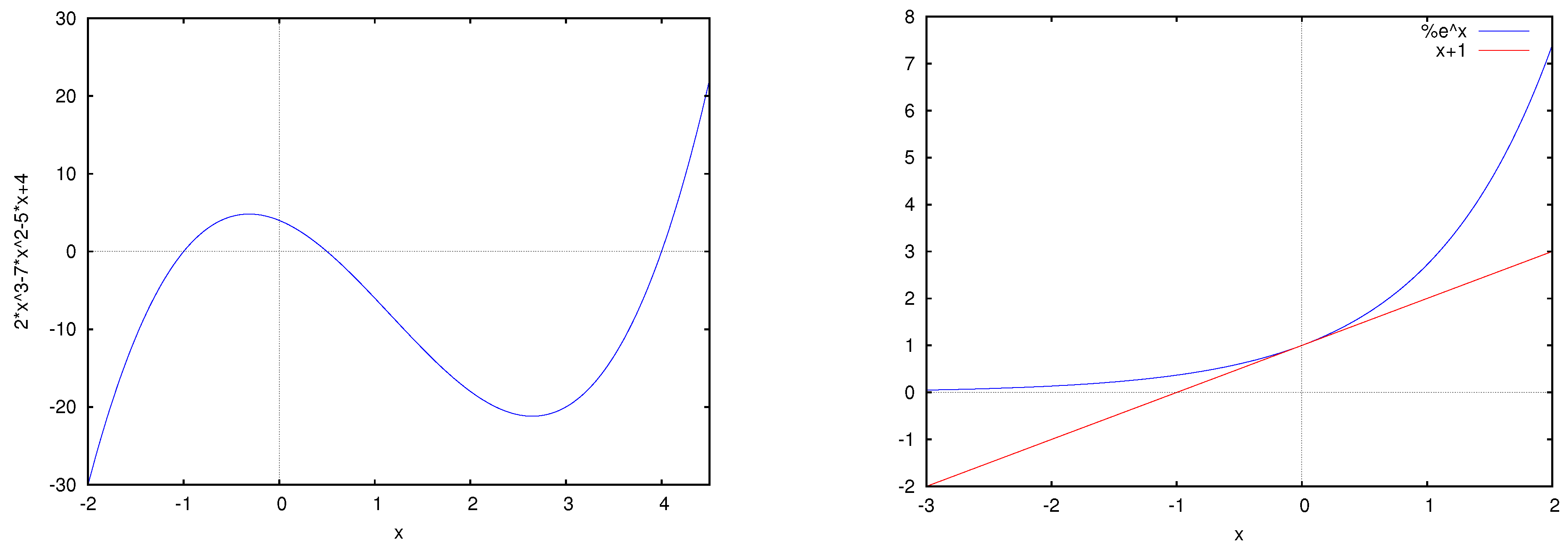
(%i8) plot2d(2*x^3-7*x^2-5*x+4, [x,-2,4.5]);	(Figure 1, left panel)
(%i9) plot2d([exp(x), 1 + x], [x,-3,2]);	(Figure 1, right panel)

displays the wxMaxima command inputs and their corresponding outputs. Our experience as instructors suggests that wxMaxima is also handy for obtaining quick and excellent-quality graphical plots, particularly three-dimensional objects that can be hard to sketch manually. In turn, this visualization enhances students’ understanding of applying Calculus concepts.

Example 2.

Sketching functions (2D plots):

$$\begin{array}{cccc}\hfill y=f\left(x\right)& =2x^3-7x^2-5x+4\hfill & \hfill & [\mathit{cubic} \mathit{function}]\hfill \\ \hfill y=g\left(x\right)& =e^x\mathrm{and}L\left(x\right)=1+x\hfill & \hfill & [\mathit{exponential} \mathit{function} \mathit{and} \mathit{its} \mathit{linear} \mathit{approximation}].\hfill \end{array}$$

Example 2 gives examples of generating 2D plots of a single polynomial function and an exponential function together with the corresponding linear approximation. Table 2 shows the wxMaxima command inputs, and Figure 1 displays the corresponding outputs. The plot on the left-hand side can be used to verify the theoretical computation of the local extrema, increasing or decreasing test, and concavity test to a cubic function $f\left(x\right)=2x^3-7x^2-5x+4$. The plot on the right-hand side shows a linear approximation $L\left(x\right)$ of an exponential function $g\left(x\right)=e^x$ at $x=0$. The sketching quality in wxMaxima is remarkably excellent, and the task is completed swiftly. SageMath is rather slow to produce plots, and WolframAlpha’s free version generates poor quality plots.

Example 3.

2D and 3D parametric plots:

$$\begin{array}{ccc}r\left(t\right)=1-sint,\hfill & 0\le t\le 2\pi \hfill & \left[\mathit{cardioid}\right]\hfill \\ \mathit{r}\left(t\right)=\langle cost,sint,t\rangle ,\hfill & 0\le t\le 5\pi \hfill & \left[\mathit{helix}\right].\hfill \end{array}$$

Example 3 gives illustrations of parametric plots in both 2D plane and 3D space. The wxMaxima input commands and their corresponding outputs are presented in

Table 3. Examples of wxMaxima commands and their corresponding outputs showing 2D and 3D plots of parametric curves cardioid and helix, respectively, and their corresponding arc lengths.

Input	Output
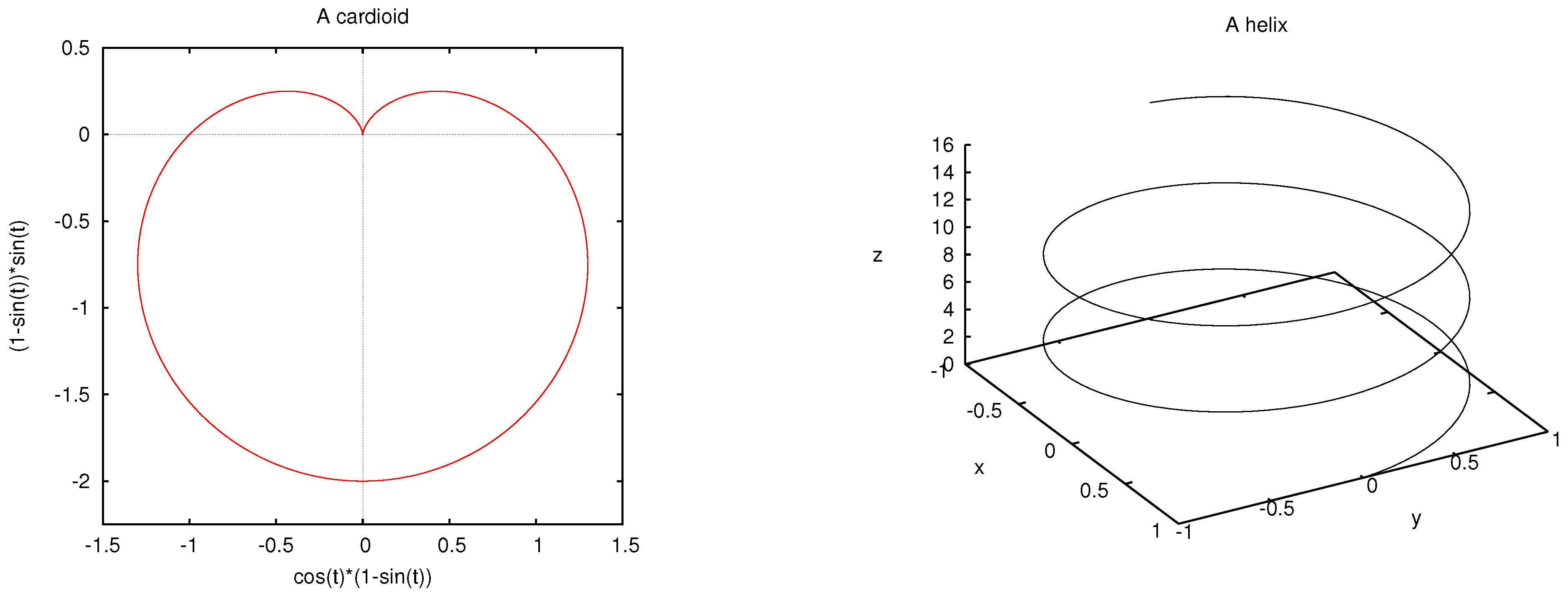
(%i10) r: 1 - sin(t);	(r) $1-sin\left(t\right)$
(%i11) plot2d([parametric,r*cos(t),r*sin(t)],	(Figure 2,
[t,0,2*%pi],[color,red],[x,-1.5,1.5],	left panel)
[y,-2.25,0.5],same_xy,[title,"A cardioid"]);
(%i12) integrate(1/2*r^2,t,0,2*%pi);	${\displaystyle \frac{3\pi }{2}}$
(%i13) plot3d([cos(t),sin(t),t],[t,0,5*%pi],[y,-1,1],
[grid,100,2],[gnuplot_pm3d,true],[elevation,50],	(Figure 2,
[azimuth,60],[legend,false],[title,"A helix"]);	right panel)
(%i14) factor(integrate(sqrt(diff(cos(t),t)^2
+diff(sin(t),t)^2+diff(t,t)^2),t,0,5*%pi));	$5\sqrt{2}\pi$

. A 2D plot of the polar curve cardioid $r\left(t\right)=1-sint$, $0\le t\le 2\pi$, and a 3D plot of helix $\mathit{r}\left(t\right)=\langle cost,sint,t\rangle$, $0\le t\le 5\pi$ are given on the left and right panels of Figure 2, respectively.

Two of integral applications are calculating the area enclosed by a polar curve and the arc length of a parametric curve. The commands to calculate the area A enclosed by the cardioid and the length of the helix L and their corresponding results are also given in Table 3. Mathematically, they are performed as follows, where the prime denotes differentiation with respect to t:

$$\begin{array}{cc}\hfill A& ={\int }_0^{2\pi }\frac{1}{2}{r}^{2}dt={\int }_0^{2\pi }\frac{1}{2}{(1-sint)}^{2}dt=\frac{3\pi }{2}\hfill \\ \hfill L& ={\int }_0^{5\pi }\sqrt{x^{\prime }{\left(t\right)}^2+y^{\prime }{\left(t\right)}^2+z^{\prime }{\left(t\right)}^2}dt={\int }_0^{5\pi }\sqrt{{sin}^{2}t+{cos}^{2}t+1}dt=5\sqrt{2}\pi .\hfill \end{array}$$

Example 4.

3D surfaces of Möbius band and torus:

$$\begin{array}{cccc}\hfill \mathit{s}(x,y)& =〈\left(3+ycos\frac{x}{2}\right)cosx,\left(3+ycos\frac{x}{2}\right)sinx,ysin\frac{x}{2}〉\hfill & \hfill & \left[Mö\mathit{bius}\mathit{band}\right]\hfill \\ \hfill \mathit{t}(\theta ,\varphi )& =\langle (2+cos\theta )cos\varphi ,(2+cos\theta )sin\varphi ,sin\theta \rangle ,0\le \theta ,\varphi <2\pi .\hfill & \hfill & \left[\mathit{torus}\right]\hfill \end{array}$$

The wxMaxima input commands and their corresponding outputs are given in

Table 4. Examples of wxMaxima commands and their corresponding outputs showing 3D plots of parametric surfaces Möbius band and torus.

Input	Output
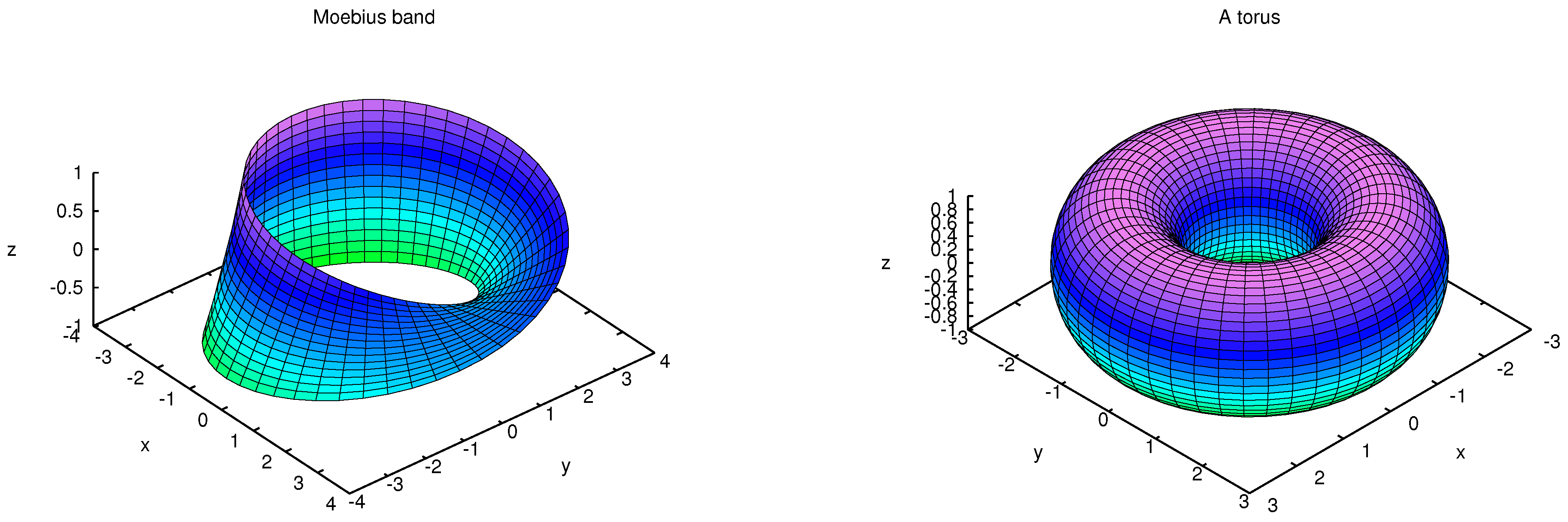
(%i15) plot3d([cos(x)*(3+y*cos(x/2)),sin(x)*(3+y*cos(x/2)),
y*sin(x/2)],[x,-%pi,%pi],[y,-1,1],[’grid,50,15],	(Figure 3,
[legend,false],[elevation,35],[azimuth,50],	left panel)
[title,"Moebius band"]);
(%i16) plot3d([cos(y)*(2+cos(x)),sin(y)*(2+cos(x)),sin(x)],
[x,0,2*%pi],[y,0,2*%pi],[gnuplot_pm3d,true],	(Figure 3,
[grid,50,50],[legend,false],[elevation,30],	right panel)
[azimuth,135],[title,"A torus"]);

and Figure 3, respectively. Three-dimensional plots such as this Möbius band and torus can be rotated easily in any direction. Sometimes also called the Möbius strip, the former is a surface with only one side and only one boundary curve, the simplest example of a nonorientable surface. All Möbius bands have a twofold symmetry rotational axis, for which a 180° rotation results in strips indistinguishable from the original. The surface finds abundant applications in physical sciences, including nanostructures [16], metamaterials [17], polymeric materials [18], and photonic crystals [19].

The torus example comes from the problem of calculating the volume of solid revolution. It is obtained from a disk ${(x-2)}^2+z^2\le 1$ revolved about the z-axis, and thus, it is radially symmetric about the z-axis. The desired viewpoint can be obtained easily by setting the elevation and azimuth angles. This is beneficial in comparison to the Matlab plots where figures usually have a high number of pixels and are rather heavy to be rotated. Although the surface of revolution is a fascinating object among geometers and topologists, it also finds ample applications in nanophotonics [20], metamaterials [21], magnetized plasma [22], and polymer chemistry [23].

2.2. wxMaxima’s Weaknesses

In this subsection, we consider several examples where wxMaxima is deficient. When sketching a function with singularities, we can discern an improved plot by including supplementary commands. The CAS wxMaxima is not particularly strong when it comes to evaluating integrals, particularly the integral of rational functions. This may come as a surprise since the latter are commonplace and considered to be schematically viable.

Example 5.

A sketch of ${\displaystyle y=f\left(x\right)=\frac{x^2}{x^2-1}}$.

In this example, sketching a 2D plot of a function with vertical asymptotes requires an additional instruction. Although the output from “plot2d(x^2/(x^2-1),[x,-4,4]);” input shows that there are two vertical asymptotes at $x=\pm 1$, modifying the input produces a better visibility, cf. [24]:

“plot2d(max(min(x^2/(x^2-1),10),-10),[x,-4,4]);”. Figure 4 compares the 2D plots obtained from these two inputs.

Example 6.

Indefinite and definite integrals involving trigonometric functions:

$$\int \frac{xsinx}{1+{cos}^{2}x}dxand{\int }_0^{\pi }\frac{xsinx}{1+{cos}^{2}x}dx.$$

Both wxMaxima and Matlab fail to evaluate both integrals. The indefinite integral above involves a non-elementary function Li${}_2\left(z\right)$. Special function Li${}_s\left(z\right)$ is a polylogarithm of order s and argument z. It is also known as the Jonquière’s function and is defined by a power series in z; it is also a Dirichlet series in s:

$${\mathrm{Li}}_s\left(z\right)=\sum _{k=1}^{\infty }\frac{z^k}{k^s}.$$

Both WolframAlpha and Mathematica can produce a correct answer for the above definite integral: ${\pi }^2/4$. Although treatment of the indefinite integral is beyond the Calculus course, the definite integral can be evaluated using a simple substitution rule. Appendix A shows how to evaluate it without any help from CAS.

Example 7.

Gärtner’s indefinite integral of a rational function [25]:

$$\int \frac{\sqrt{2}dx}{{(x-1)}^4+\frac{1}{16}}.$$

When employing the “integrate(sqrt(2)/((x-1)^4+1/16),x);” command, wxMaxima could not directly handle this integral. However, using the substitution $y=x-1$: “changevar(%,x-1-y,y,x);”, the integral transforms into

$$\int \frac{16\sqrt{2}dy}{16y^4+1}.$$

Asking wxMaxima to evaluate the integral, “ev(%,integrate);”, we obtain

$$2log(4y^2+2\sqrt{2}y+1)-2log(4y^2-2\sqrt{2}y+1)+4atan\left(\frac{4y+\sqrt{2}}{\sqrt{2}}\right)+4atan\left(\frac{4y-\sqrt{2}}{\sqrt{2}}\right).$$

Substituting back to the original variable gives us the desired integral, “sfx: %,y=x-1”:

$$\begin{array}{cc}\hfill & 2log>(4{(x-1)}^2+2\sqrt{2}(x-1)+1>)-2log>(4{(x-1)}^2-2\sqrt{2}(x-1)+1)\hfill \\ \hfill & +4atan\left(\frac{4(x-1)+\sqrt{2}}{\sqrt{2}}\right)+4atan\left(\frac{4(x-1)-\sqrt{2}}{\sqrt{2}}\right).\hfill \end{array}$$

In attempting to solve indefinite integrals of rational functions, wxMaxima essentially still uses the algorithms that were described by Moses [26]. The CAS employs the classical algorithmic tool in symbolic integration known as Hermite reduction. Both Hermite and Ostrogradsky demonstrated decomposing indefinite integral of rational functions as the sum of a function with simple poles and the derivative of another rational function, i.e., for $R\in \mathbb{Q}\left(x\right)$

$$\int R(x)dx=U(x)+\int A(x)dx,U,A\in \mathbb{Q}(x)$$

where A has only simple poles and vanishes at infinity [27,28,29,30].

Thus, wxMaxima implements the combination of Hermite reduction with either the partial fraction decomposition (Bernoulli–Leibniz algorithm) to compute the rational part of the integrand or with some heuristic methods in computing its transcendental parts for several easier cases. Although other commercial software such as Axiom and 3M might also implement integration using Hermite reduction for the rational part of the integrand, it employs more contemporary and advanced methods to integrate the remaining terms after Hermite reduction is implemented.

Example 8.

Bronstein’s definite integral of a rational function [31]:

$${\int }_1^2\frac{x^4-3x^2+6}{x^6-5x^4+5x^2+4}dx.$$

When we attempt the command “integrate((x^4-3*x^2+6)/(x^6-5*x^4+5*x^2+4), x,1,2);”, wxMaxima could not compute this integral. However, Axiom and 3M can tackle it. Axiom’s output reads:

$$\frac{2atan\left(8\right)+2atan\left(5\right)+2atan\left(2\right)+2atan\left(\frac{1}{2}\right)-\pi }{2}.$$

Maple’s output is given as follows:

$$arctan\left(\frac{1}{2}\right)-\frac{1}{2}\pi +arctan\left(5\right)+arctan\left(8\right)+arctan\left(2\right).$$

Interestingly, Mathematica and Matlab give the following outputs, respectively, which were simpler than the ones from the previous two software:

$$\frac{5}{4}\pi -arctan\left(2\right)\mathrm{and}\pi -arctan(1/3).$$

All of these results correspond to an identical numerical value of approximately $2.819842$. The proof is shown in Appendix B.1.

It would also be interesting to observe the corresponding indefinite integral. While wxMaxima anticipatedly cannot compute the indefinite integral, Axiom, Maple, and Matlab delivered the same results and agreed with Formula (2.20) in [31]. This reads

$$\int \frac{x^4-3x^2+6}{x^6-5x^4+5x^2+4}dx=arctan\left(x\right)+arctan\left(x^3\right)+arctan\left(\frac{x^5-3x^3+x}{2}\right)+C.$$

In particular, Mathematica is of special interest as the output of the corresponding indefinite integral does not agree with the formula given in [31]. It reads as follows (some terms were rearranged):

$$\int \frac{x^4-3x^2+6}{x^6-5x^4+5x^2+4}dx=\frac{1}{2}arctan\left[\frac{x(x^2-3)}{x^2-2}\right]-\frac{1}{2}arctan\left[\frac{x(x^2-3)}{2-x^2}\right]+C.$$

The definite integral is given as follows:

$$\begin{array}{cc}\hfill {\int }_1^2\frac{x^4-3x^2+6}{x^6-5x^4+5x^2+4}dx& =\underset{t\to {\sqrt{2}}^{-}}{lim}\left\{\frac{1}{2}arctan\left[\frac{x(x^2-3)}{x^2-2}\right]-\frac{1}{2}arctan\left[\frac{x(x^2-3)}{2-x^2}\right]\right\}-arctan\left(2\right)\hfill \\ \hfill & +arctan\left(1\right)-\underset{t\to {\sqrt{2}}^{+}}{lim}\left\{\frac{1}{2}arctan\left[\frac{x(x^2-3)}{x^2-2}\right]-\frac{1}{2}arctan\left[\frac{x(x^2-3)}{2-x^2}\right]\right\}\hfill \\ \hfill & =\left(\frac{\pi }{2}-arctan\left(2\right)\right)+\left(\frac{\pi }{4}+\frac{\pi }{2}\right)=\frac{5}{4}\pi -arctan\left(2\right).\hfill \end{array}$$

The first and second chapters of [31] explain outline algorithms for the integration of rational functions in great detail. All relevant algorithms are given in pseudocodes. With an estimated effort of 500 to 700 lines of code, these algorithms can be implemented in wxMaxima.

Example 9.

Adamchik’s definite integral of a rational function [32]:

$${\int }_0^4\frac{x^2+2x+4}{x^4-7x^2+2x+17}dx.$$

For an indefinite integral, wxMaxima could not compute it. Other software, namely, Axiom, Maple, and Matlab, presented an identical solution but with rather dissimilar expressions:

$$\int \frac{x^2+2x+4}{x^4-7x^2+2x+17}dx=arctan(x-1)+arctan\left(\frac{1}{3}{x}^3-\frac{1}{2}{x}^2-x+\frac{5}{3}\right)+C.$$

On the other hand, the computational result from Mathematica produced an antiderivative expression with discontinuities at $x=\pm 2$:

$$\int \frac{x^2+2x+4}{x^4-7x^2+2x+17}dx=\frac{1}{2}arctan\left(\frac{-x-1}{x^2-4}\right)-\frac{1}{2}arctan\left(\frac{x+1}{x^2-4}\right)+C.$$

For the definite integral, while all numerical results agree, the symbolic outputs yield remarkably distinct expressions. The outputs are given as follows:

$$\begin{array}{cccc}\hfill {\int }_0^4\frac{x^2+2x+4}{x^4-7x^2+2x+17}dx& =\frac{\pi }{4}+arctan\left(3\right)-arctan\left(\frac{5}{3}\right)+arctan\left(\frac{41}{3}\right)\hfill & \hfill & [\mathit{Axiom}\mathrm{and}\mathit{Maple}]\hfill \\ \hfill & =\frac{5}{4}\pi -arctan\left(\frac{75}{11}\right)\hfill & \hfill & [\mathit{Matlab}]\hfill \\ \hfill & =\pi -arctan\left(\frac{1}{4}\right)-arctan\left(\frac{5}{12}\right)\hfill & \hfill & [\mathit{Mathematica}]\hfill \\ \hfill & =\left(\mathrm{a}\mathrm{tedious}\mathrm{and}\mathrm{complicated}\mathrm{expression}\right)\hfill & \hfill & [\mathit{wxMaxima}]\hfill \\ \hfill & \approx 2.50182\hfill & \hfill & [\mathrm{numerical}\mathrm{value}].\hfill \end{array}$$

Although wxMaxima computes and produces an output for the definite integral, that expression is exceptionally tedious and complicated. It is also unclear how it was obtained, but possibly by performing a contour integration. Despite that tiresome and intricate expression, its numerical evaluation yields a value that agrees with the one calculated by other software. A high floating-point precision command, e.g., “fpprec:150” needs to be imposed to obtain that numerical value. Except for the exact wxMaxima output, Appendix B.2 verifies that the above outputs had identical values.

Similar to Example 8, when we want to use Mathematica’s antiderivative result to compute the value of the definite integral, we need to split the interval of integration at the point of discontinuity to avoid a wrong result of ${\displaystyle -arctan\left(\frac{1}{4}\right)-arctan\left(\frac{5}{12}\right)}$. The computational summary is given as follows:

$$\begin{array}{cc}\hfill {\int }_0^4\frac{x^2+2x+4}{x^4-7x^2+2x+17}dx& =\underset{t\to 2^{-}}{lim}\left\{\frac{1}{2}arctan\left(\frac{-t-1}{t^2-4}\right)-\frac{1}{2}arctan\left(\frac{t+1}{t^2-4}\right)\right\}-arctan\left(\frac{1}{4}\right)\hfill \\ \hfill & -arctan\left(\frac{5}{12}\right)-\underset{t\to 2^{+}}{lim}\left\{\frac{1}{2}arctan\left(\frac{-t-1}{t^2-4}\right)-\frac{1}{2}arctan\left(\frac{t+1}{t^2-4}\right)\right\}\hfill \\ \hfill & =\left[\frac{\pi }{2}-arctan\left(\frac{1}{4}\right)\right]-\left[arctan\left(\frac{5}{12}\right)-\frac{\pi }{2}\right]\hfill \\ \hfill & =\pi -arctan\left(\frac{1}{4}\right)-arctan\left(\frac{5}{12}\right).\hfill \end{array}$$

Example 10.

Tobey’s indefinite integral of a rational function [33]:

$$\int \frac{7x^{13}+10x^8+4x^7-7x^6-4x^3-4x^2+3x+3}{x^{14}-2x^8-2x^7-2x^4-4x^3-x^2+2x+1}dx.$$

Except for wxMaxima, all other CAS can compute this integral. The result can be found on page 502 of [34] using the Rothstein–Trager method. It reads

$$\frac{1}{2}(1+\sqrt{2})log\left(x^7-\sqrt{2}{x}^2-(1+\sqrt{2})x-1\right)+\frac{1}{2}(1-\sqrt{2})log\left(x^7+\sqrt{2}{x}^2-(1-\sqrt{2})x-1\right)+C.$$

3. Discussion

3.1. wxMaxima in Perspective

There exists a distinct paradigm between the CAS mentioned in the Introduction. While Matlab is particularly strong in numerical computation, the real forte of wxMaxima, Maple, and Mathematica is symbolic computation. Matlab has also incorporated some symbolic features, and the latter three can also perform numerical computations as well.

When it comes to symbolic functionality, wxMaxima still has a long way to go to catch up other commercial software. Together with Axiom and SageMath, a formula editor is missing in Maxima, although wxMaxima serves efficiently as its user interface. While Axiom does not possess graph-theory symbolic functionality, wxMaxima does. Unfortunately, Diophantine equation solvers and quantifier elimination are absent in wxMaxima, and SageMath acquires these two features via SymPy and qepcad optional packages, respectively.

Table 5. A summary of significantly developed symbolic functionality among various software. Maxima has a shortfall in quantifier elimination and Diophantine equation solver. The missing formula editor can be overcome by a user interface wxMaxima.

Software	Formula Editor	Calculus		Quantifier Elimination	Solvers
		Integration	Integral Transforms		Inequalities	Diophantine Equations	Differential Equations	Recurrence Relations
Axiom	✗	✓	✓	✓	✓	✓	✓	✓
Magma	✗	✗	✗	✗	✓	✗	✗	✗
Maple	✓	✓	✓	✓	✓	✓	✓	✓
Mathematica	✓	✓	✓	✓	✓	✓	✓	✓
Maxima	✗	✓	✓	✗	✓	✗	✓	✓
Matlab	✓	✓	✓	✓	✓	✗	✓	✗
SageMath	✗	✓	✓	✓	✓	✓	✓	✓

summarizes the significantly developed symbolic functionality in various software systems.

An important feature of wxMaxima that trumps other CAS is the admittance of referring to the result of the last evaluated expression with a percentage sign (%). Although we may organize the commands in spatial order, wxMaxima stores information in chronological order. Thus, the % always refers to the most recently executed command, and not necessarily to the one that appears directly above the executed command [11]. As already mentioned in the Introduction, since wxMaxima is open-source software, it is maintained by an active community of developers, and thus being updated regularly. New releases occur approximately twice annually. For a proprietary software like 3M, not everyone can inspect, modify, or enhance, but only a team of developers from the company or organization who maintains exclusive control over it can modify the software. Admittedly, the most important reason for utilizing wxMaxima, both in teaching and research is the cost, and many authors agreed on this particular notable reason [10,11,12].

3.2. Educational Benefit

There are many educational benefits of embedding CAS wxMaxima into teaching and learning, Calculus in particular, and mathematics in general. The software serves as meaningful assistance not only to students but also to instructors in verifying hand-computed results, obtaining numerical values of tedious expressions, and providing rich-quality graphical plots. Hence, the benefit of algebraic, numerical, and graphical aspects, respectively. The time reduction gained in the labor of manual calculation can be spent for a deeper understanding of key ideas, theoretical concepts, and problem-solving methods.

Some examples discussed in Section 2 support this testimony. By observing the graph of a cubic function, students should establish a connection between the visual plot and the computational result of obtaining intervals where the function is increasing, decreasing, concave up, and concave down. Other features, such as the local maxima and minima, and inflection points should follow naturally. By examining the linear approximation of a function, students should be able to conclude why the approximation works for the variable x near a specified point of interest. At an advanced level, this comprehension is advantageous for linear-stability analysis.

The literature does not lack in supplying educational benefits of using CAS in mathematics lessons. From a coding perspective, the programming language in wxMaxima flows more naturally in comparison to that in other software, and hence allows for students to autonomously implement simple algorithms [4]. For current and future calculus teachers, wxMaxima could reduce the time spent on course preparation [7]. By allowing students to induce judgments and make mistakes, the adoption of wxMaxima stimulates the interactive-learning process through testing, evaluation, decision-making, and error correction [9]. Weigand argued that the wise use of CAS could foster students’ ability in problem solving, modeling, proving, and communicating [35]. The CAS can even be blended with an innovative pedagogical approach, such as flipped classrooms [36].

Additional benefits come along as more instructors adopt and implement a CAS, particularly wxMaxima, into their teaching and learning. However, wxMaxima is not a perfect software, as we elaborated through several examples in Section 2.

3.3. Limitation

This study admits several limitations. First, the extent of course materials in Single-Variable Calculus (SVC) is overwhelmingly profuse while the time is scanty. It covers nine chapters of Stewart’s Calculus textbook [37], and they need to be completed in 14 weeks. Embedding technology into teaching and learning contributes an additional burden. In a typical North American university, similar content would be covered in two different courses for two consecutive semesters. Usually called “Calculus 1” and “Calculus 2”, they cover Differential and Integral Calculus, respectively. The latter often includes an Introduction to Differential Equations, and Sequence and Series. Hence, teaching Calculus using wxMaxima with less material coverage seems to be a promising attempt, as we could pursue in MVC.

Second, despite the superior features of wxMaxima and its specialty in symbolic operations, the CAS itself has some weaknesses that could be challenging for beginners to learn, adopt, and adapt, both as instructors and students, where it might be more conspicuous for the latter. The CAS is admittedly far from perfect due to the nature of free and open-source software. Other commercial CAS such as Mathematica and Maple might be better since the companies that release them possess an army of paid personnel working around the clock to improve the software. Nevertheless, we are not without hope since wxMaxima is updated frequently, bugs are fixed, and documentation is improved by a group of volunteer developers who work tirelessly.

4. Conclusions

In this article, we considered several features of wxMaxima that could be useful for enhancing the quality of Calculus teaching and learning. Although the CAS itself is far from perfect, focusing on its strengths might benefit both students and instructors when embedding the software into the subject. We included some examples where wxMaxima assists well in understanding Calculus concepts better. These include calculating limit, finding a derivative of a function, evaluating definite and indefinite integrals, generating plots for explicit functions, parametric functions, polar curves, and three-dimensional objects. The visualization aspect enhances excellent teaching.

For teachers and instructors who are currently adopting Maple or Mathematica in their teaching, we are interested in stimulating a discussion on whether it is viable to integrate, or even switch entirely, to wxMaxima. This endeavor is not beyond our reach, at least for a sequence of Calculus courses (PreCalculus, SVC, and MVC).

For Linear Algebra, Matlab is still the most popular software among both engineers and educators thanks to its many professional contributors, rigorous development, powerful numerical computation, and additional package Simulink. SageMath is also becoming popular for Linear Algebra teaching and learning since it utilizes existing open-source libraries specifically designed for Linear Algebra, including LAPack and NumPy. Since wxMaxima also possesses many functions for manipulating matrices, we would not be too ambitious to persuade educational practitioners by considering to switch CAS to wxMaxima for Linear Algebra teaching and learning. Some Linear Algebra problems are worth testing using wxMaxima nonetheless.

Despite the many admirable qualities of wxMaxima, our experience in other courses and with different CAS suggests that some students hate when instructors generally attempt to embed any CAS in general into mathematics teaching and learning. For example, after implementing Calculus with SageMath in 2012, some students provided feedback suggesting to eliminate SageMath from Calculus teaching. For Linear Algebra, a dedicated one-hour problem-solving session using Matlab was not favored among the students. Students’ feedback on teaching evaluation consistently mentions that the computer laboratory sessions are a waste of time and must be replaced by the traditional problem-solving sessions using pen and paper.

From our experience of embedding wxMaxima into Calculus courses, both Single-Variable and Multivariable, very few students gave positive feedback regarding the software. The majority of students’ comments voice an atmosphere of negativity and resistance, they tend to push away wxMaxima. Even if they seem to embrace the CAS favorably, they might forget it as soon as the semester is over. In subsequent courses, their instructors might not use wxMaxima anymore. There are other important programming languages (e.g., Python, C++, and Java) that students could master before they enter the job market.

References

- Maxima Website Page. Available online: https://maxima.sourceforge.io/ (accessed on 7 June 2021).
- SourceForge Website Page Hosting Maxima Executable File for Windows. Available online: http://sourceforge.net/projects/maxima/files/Maxima-Windows/ (accessed on 7 June 2021).
- Ayub, M.; Fauzi, A.; Ahmad Tarmizi, R.; Abu Bakar, K.; Wong, S.L. Adoption of Wxmaxima software in the classroom: Effect on students’ motivation and learning of mathematics. Malays. J. Math. Sci. 2014, 8, 311–323. [Google Scholar]
- García, A.; García, F.; Rodríguez, G.; de la Villa, A. Could it be possible to replace DERIVE with MAXIMA? Int. J. Technol. Math. Educ. 2011, 18, 137–142. [Google Scholar]
- Díaz, A.; García, A.; de la Villa, A. An example of learning based on competences: Use of Maxima in Linear Algebra for Engineers. Int. J. Technol. Math. Educ. 2011, 18, 177–181. [Google Scholar]
- Fedriani, E.M.; Moyano, R. Using Maxima in the Mathematics Classroom. Int. J. Technol. Math. Educ. 2011, 18, 171–176. [Google Scholar]
- Velychko, V.Y.; Stopkin, A.V.; Fedorenko, O.H. Use of computer algebra system Maxima in the process of teaching future mathematics teachers. Inf. Technol. Learn. Tools 2019, 69, 112–123. [Google Scholar] [CrossRef]
- Dehl, M. Exploring Advanced Math with Maxima. Linux J. 2009. Available online: http://www.linuxjournal.com/content/exploring-advanced-math-maxima (accessed on 7 June 2021).
- Žáková, K. Maxima–An open alternative for engineering education. In Proceedings of the Global Engineering Education Conference (EDUCON), Amman, Jordan, 4–6 April 2011; pp. 1022–1025. [Google Scholar]
- Hannan, Z. wxMaxima for Calculus I. wxMaxima for Calculus II; Solano Community College: Fairfield, CA, USA, 2015; Available online: https://wxmaximafor.wordpress.com/ (accessed on 7 June 2021).
- Timberlake, T.K.; Mixon, J.W. Classical Mechanics with Maxima; Springer: New York, NY, USA, 2016. [Google Scholar]
- Senese, F. Symbolic Mathematics for Chemists: A Guide for Maxima Users; John Wiley & Sons: Hoboken, NJ, USA, 2019. [Google Scholar]
- Woollett, E.L. Maxima by Example; California State University: Long Beach, CA, USA, 2020; Available online: https://web.csulb.edu/~woollett/mbe.html (accessed on 7 June 2021).
- Puentedura, R.R. Symbolic Math–A Workflow; Hippasus: Williamstown, MA, USA, 2020; Available online: http://www.hippasus.com/resources/symmath/index.html (accessed on 7 June 2021).
- Karjanto, N.; Husain, H.S. Adopting Maxima as an open-source Computer Algebra System into mathematics teaching and learning. In Proceedings of the 13th International Congress on Mathematical Education; Kaiser, G., Ed.; Springer: Cham, Switzerland, 2017; pp. 733–734. [Google Scholar]
- Starostin, E.L.; Van Der Heijden, G.H.M. The shape of a Möbius strip. Nat. Mater. 2007, 6, 563–567. [Google Scholar] [CrossRef] [PubMed]
- Chang, C.W.; Liu, M.; Nam, S.; Zhang, S.; Liu, Y.; Bartal, G.; Zhang, X. Optical Möbius symmetry in metamaterials. Phys. Rev. Lett. 2010, 105, 235501. [Google Scholar] [CrossRef] [PubMed]
- Nie, Z.Z.; Zuo, B.; Wang, M.; Huang, S.; Chen, X.M.; Liu, Z.Y.; Yang, H. Light-driven continuous rotating Möbius strip actuators. Nat. Commun. 2021, 12, 1–10. [Google Scholar] [CrossRef] [PubMed]
- Han, Y.; He, A.L.; Chen, H.J.; Liu, S.Y.; Lin, Z.F. Photonic states on Möbius band. J. Opt. 2020, 22, 035103. [Google Scholar] [CrossRef]
- Ahmadiv, A.; Gerislioglu, B.; Ahuja, R.; Mishra, Y.K. Toroidal metaphotonics and metadevices. Laser Photonics Rev. 2020, 14, 1900326. [Google Scholar] [CrossRef]
- Kaelberer, T.; Fedotov, V.A.; Papasimakis, N.; Tsai, D.P.; Zheludev, N.I. Toroidal dipolar response in a metamaterial. Science 2010, 330, 1510–1512. [Google Scholar] [CrossRef] [PubMed] [Green Version]
- Kliem, B.; Török, T. Torus instability. Phys. Rev. Lett. 2006, 96, 255002. [Google Scholar] [CrossRef] [PubMed] [Green Version]
- Pochan, D.J.; Chen, Z.; Cui, H.; Hales, K.; Qi, K.; Wooley, K.L. Toroidal triblock copolymer assemblies. Science 2004, 306, 94–97. [Google Scholar] [CrossRef]
- Glasner, M.A. Maxima Guide for Calculus Students; Pennsylvania State University: University Park, PA, USA, 2004; Available online: http://michel.gosse.free.fr/documentation/fichiers/maxima_sg.pdf (accessed on 7 June 2021).
- Gärtner, B. The Computer Algebra Program Maxima–A Tutorial; Bildungsgüter: München, Germany, 2005; Available online: http://www.bildungsgueter.de/MaximaEN/Contents.htm (accessed on 7 June 2021).
- Moses, J. Symbolic integration: The Stormy Decade. Commun. Acm 1971, 14, 548–560. [Google Scholar] [CrossRef] [Green Version]
- Subramaniam, T.N.; Malm, D.E. How to integrate rational functions. Am. Math. Mon. 1992, 99, 762–772. [Google Scholar] [CrossRef]
- Bostan, A.; Chen, S.; Chyzak, F.; Li, Z.; Xin, G. Hermite reduction and creative telescoping for hyperexponential functions. In Proceedings of the 38th International Symposium on Symbolic and Algebraic Computation, Boston, MA, USA, 26–29 June 2013; pp. 77–84. [Google Scholar]
- Bostan, A.; Chyzak, F.; Lairez, P.; Salvy, B. Generalized Hermite reduction, creative telescoping and definite integration of D-finite functions. In Proceedings of the 2018 ACM International Symposium on Symbolic and Algebraic Computation, New York, NY, USA, 16–19 July 2018; pp. 95–102. [Google Scholar]
- Moir, R.H.; Corless, R.M.; Maza, M.M.; Xie, N. Symbolic-numeric integration of rational functions. Numer. Algorithms 2020, 83, 1295–1320. [Google Scholar] [CrossRef] [Green Version]
- Bronstein, M. Symbolic Integration I: Transcendental Functions, 2nd ed.; Springer: Berlin/Heildelberg, Germany, 2005. [Google Scholar]
- Adamchik, V.S. Definite Integration in Mathematica V3.0.; Preprint; Carnegie Melon University: Pittsburgh, PA, USA, 2008; p. 18. Available online: https://kilthub.cmu.edu/articles/journal_contribution/Definite_Integration_in_Mathematica_V3_0/6604700 (accessed on 7 June 2021). [CrossRef]
- Tobey, R.G. Algorithms for Antidifferentiation of Rational Functions. Ph.D. Thesis, Harvard University, Boston, MA, USA, 1967. [Google Scholar]
- Geddes, K.O.; Czapor, S.R.; Labahn, G. Algorithms for Computer Algebra; Kluwer Academic Publishers: Boston, MA, USA; Dordrecht, The Netherlands; London, UK, 1992. [Google Scholar]
- Weigand, H.G. What is or what might be the benefit of using Computer Algebra Systems in the learning and teaching of Calculus? In Innovation and Technology Enhancing Mathematics Education; Faggiano, E., Ferrara, F., Montone, A., Eds.; Springer: Cham, Switzerland, 2017; pp. 161–193. [Google Scholar]
- Karjanto, N.; Simon, L. English-medium instruction Calculus in Confucian-Heritage Culture: Flipping the class or overriding the culture? Stud. Educ. Eval. 2019, 63, 122–135. [Google Scholar] [CrossRef]
- Stewart, J. Calculus: Early Transcendentals for Scientists and Engineers, Metric Edition; Cengage Learning: Singapore, 2017. [Google Scholar]