A Comparative Analysis of Simulated Annealing and Variable Neighborhood Search in the ATCo Work-Shift Scheduling Problem

Abstract

This paper deals with the air traffic controller (ATCo) work shift scheduling problem. This is a multi-objective optimization problem, as it involves identifying the best possible distribution of ATCo work and rest periods and positions, ATCo workload and control center changes in order to cover an airspace sector configuration, while, at the same time, complying with ATCo working conditions. We propose a three-phase problem-solving methodology based on the variable neighborhood search (VNS) to tackle this problem. The solution structure should resemble the previous template-based solution. Initial infeasible solutions are built using a template-based heuristic in Phase 1. Then, VNS is conducted in Phase 2 in order to arrive at a feasible solution. This constitutes the starting point of a new search process carried out in Phase 3 to derive an optimal solution based on a weighted sum fitness function. We analyzed the performance in the proposed methodology of VNS against simulated annealing, as well as the use of regular expressions compared with the implementation in the code to verify the feasibility of the analyzed solutions, taking into account four representative and complex instances of the problem corresponding to different airspace sectorings.

1. Introduction

The key concept at the heart of air traffic management (ATM) network operations is air traffic flow and capacity management (ATFCM). ATFCM should optimize traffic flows so that airlines can operate safe and efficient flights depending on air traffic control capacity. In Europe, the network manager operations center (NMOC) constantly monitors the balance between the airspace capacity and traffic load. NMOC activities are divided into four –strategic, pre-tactical, tactical and post-operational– phases [1].

The strategic phase is related to capacity prediction at ATC centers by air navigation service providers (ANSPs). ANSPs prepare a routing scheme with the help of NMOC seven days ahead of operations.

The pre-tactical phase is related to the definition of the initial network plan. The NMOC publishes the agreed plan for the day of operations, informing ATC units and aircraft operators about the ATFCM measures affecting European airspace from one to six days ahead of operations.

The tactical phase updates the plan for the day of operations according to real-time traffic demand where the NMOC monitors the situation and continuously optimizes capacity. Delays are minimized by providing aircraft affected by changes with alternative solutions on the day of operations.

The post-operational phase is related to operational process improvement by comparing planned and measured outcomes covering all ATFCM domains and units. Operational processes are measured in order to develop best practices and/or analyze lessons learned after the day of operations.

In this paper, we focus on the pre-tactical phase. This phase has to solve the very important problem of determining how the available air traffic controllers (ATCos) are assigned to each open sector to cover a sectorization structure (established in the strategic phase) for a specified amount of time. This assignment has to comply with a number of strong constraints accounting for the ATCo working conditions.

The sectorization changes throughout the day depend on aircraft traffic. More sectors are opened if the air traffic volume increases. This steps up the demand for ATCos who can only handle a limited amount of traffic.

This is a timetabling and scheduling problem. Timetabling and scheduling problems are combinatorial problems, which, on the grounds of size and complexity, cannot be solved by exact methods. For examples of other timetabling and scheduling problem-solving approaches, see [2,3].

ATCo scheduling software has already been developed within the ATM field [4]. These tools have both strengths and weaknesses [5]. Hardly any of this software has been reported in detail, sometimes because they are in-house tools. Three ATCo scheduling problem codifications were reported alongside three optimization techniques [6]. Another solution [7] is composed of a hybrid technique combining propositional satisfiability problem solving [8] and hill climbing.

A simplified version of the ATCo work shift scheduling problem for Spanish airports was solved by minimizing the number of ATCos required to cover a given airspace sectoring in compliance with Spanish ATCo working conditions [9]. The search process employs regular expressions to check solution feasibility. The solutions that output an optimal number of ATCos are used as the starting point for another optimization process targeting balanced ATCo workloads. This simplified version of the problem analyses straightforward scenarios and accounts for a core with only one type of sector for a 24-h period. Consequently, there are no constraints on ATCo distribution across sectors.

Cores including two sector types (en-route and approach sectors) and accounting for ATCos with different operating credentials were considered in [10]. This proposal focuses on the optimization of only one shift in accordance with a previously specified number of ATCos to cover a specified airspace sector configuration. This proposal adopts a multi-objective approach, accounting for ATCo work and rest periods, positions and workload distribution, the number of control center changes, and the solution structure. It proposes a three-phase problem-solving methodology. In the first phase, a template-based heuristic was used to identify unfeasible solutions. In the second phase, a number of independent simulated annealing (SA) metaheuristic runs were conducted to arrive at feasible solutions using regular expressions to check compliance with ATCo working conditions. In the third phase, simulated annealing was conducted by multiple independent runs to optimize the objective functions of the original feasible solutions again taking into account ATCo working conditions. This optimization process took into account the ordinal information on objective importance using the rank-order centroid function to transform a multiple into a single optimization problem.

In this paper, we consider the same multi-objective problem as [10], albeit using an adaptation of variable neighborhood search (VNS) rather than SA in the three-phase problem-solving methodology. Four representative and complex instances of the problem corresponding to different airspace sectorings provided by the Spanish ATM Research, Development and Innovation Reference Center (CRIDA) are now used to compare the performance of both metaheuristics in the three-phase problem-solving methodology. Moreover, the use of regular expressions to verify the ATCo labor conditions (constraints) is compared against implementation in the code in terms of execution times.

The paper is structured as follows. Section 2 describes the ATCo work-shift scheduling problem. Section 3 describes the proposed problem-solving methodology. Section 3.1 presents a template-based heuristic to identify unfeasible solutions. Then, some notions of VNS and its adaptation to the ATCo work-shift scheduling problem are provided in Section 3.2. Finally, we describe the second and third phases of the methodology aimed at reaching a feasible and an optimal solution in Section 3.3 and Section 3.4, respectively. In Section 4, four real instances are used to illustrate the proposed methodology and to compare the performance of SA against the proposed adaptation of VNS and analyze the use of regular expressions. Finally, some conclusions are provided in Section 6.

2. Problem Description

There are limits on the amount of traffic that human ATCos can handle. Therefore, air traffic conditions the number of ATCos required, as airspace sectors are created and reduced to deal with demand, resulting in varying numbers of ATCos. The sectorization of the airspace according to estimated traffic for a specified period can be defined in advance and is denoted as airspace sector configuration.

A core is composed of a set of sectors, and any one sector may belong to several cores. A control center may be responsible for managing one or more cores. Each core should be solved separately, unless there are sectors belonging to more than one core. In this case, ATCos should be simultaneously assigned to the respective cores.

There are two types of sectors: approach and en-route sectors. Depending on airport procedures, approach sectors are generally five to 10 nautical miles (9 to 18 km) from the airport, whereas en-route sectors are usually further way.

Two ATCos with different roles operate each sector. The executive ATCo communicates with aircraft, instructing pilots on how to avoid each other, whereas the planner ATCo foresees possible conflicts between aircrafts which he or she reports to the executive ATCo. ATCos are accredited to operate a particular sector and categorized as PTD or CON ATCos. A PTD ATCo can operate en-route and approach sectors, whereas a CON ATCo can only operate en-route sectors. Figure 1 is an example of an airspace sectorization for the Barcelona eastern route in Spain. Each interval is associated with a configuration (3C, 4A, 6A, …), where the number represents the number of open sectors and the letter refers to the sector configuration, i.e., there are two sectorizations with a different spatial distribution of the same number of sectors (5A and 5B in Figure 1).

Figure 1 shows one of the four examples used to illustrate our problem-solving methodology. The airspace is divided into three sectors (configuration 3C), after which one of the sectors is divided into a further two sectors. The result is configuration 4A, which is operational for one hour. The next configuration is 6A used for 40 min. See Figure 10 for further details.

A day (24 h) is divided into night (N), morning (M) and afternoon (A) periods, covered by five different ATC shifts: long morning (LMS) (5:40–14:00 h.), morning (MS) (6:20–14:00), afternoon (AS) (14:00–21:20), long afternoon (LAS) (14:00–22:20) and night (NS) (21:20–6:20). At certain times, ATCo shifts overlap: AS and LAS from 14:00 to 21:20; NS and LAS from 21:20 to 22:20, NS and LMS from 5:40 to 6:20, and MS and LMS from 6:20 to 14:00. NS ATCos are the only ATCos at work from 22:20 to 5:40.

On top of the division by shifts, ATCo working conditions also have to be taken into account. Royal Decree 1001/2010 and Law 9/2010, regulating the provision of air traffic services, stipulate these conditions, including constraints on minimum and maximum working and resting times, how long ATCos can spend in different positions, the maximum number of sectors that an ATCo can operate during a shift, etc. A list of ATCo working conditions is available in [10].

The ATCo work shift scheduling problem that we intend to solve should achieve the following objectives in accordance with a specified airspace sectorization and a specified number of ATCos with their respective accreditations:

• ATCo work and rest periods and position should respect the specified values.
• The number of control center changes should be reduced to the minimum.
• The solution structure should resemble the previous template-based solution for ease of understanding by control center staff with a view to potential manual changes.
• ATCo workload distribution should be balanced.

Experts from the Reference Center for Research, Development and Innovation in ATM (CRIDA, www.crida.es), a non-profit joint venture between ENAIRE, Spain’s air navigation manager, the Universidad Politécnica de Madrid, and Ineco, a global infrastructure engineering and consultancy leader, ranked the above objectives by importance.

3. Problem-Solving Methodology

This section outlines a three-phase methodology to solve the stated ATCo work shift scheduling problem for a given airspace sectorization. Phase 1 sets out a heuristic which is used to construct ten different initial solutions by modifying rest period lengths using an optimized template. These initial solutions require more ATCos than are available and do not satisfy all working conditions.

In Phase 2, an algorithm based on variable neighborhood search (VNS) is applied to the infeasible solutions achieved in the first phase, in order to yield a feasible solution. The aim is to reduce the number of ATCos used to meet the number of available ATCos, while penalizing the number of times labour conditions are violated until a feasible solution is achieved.

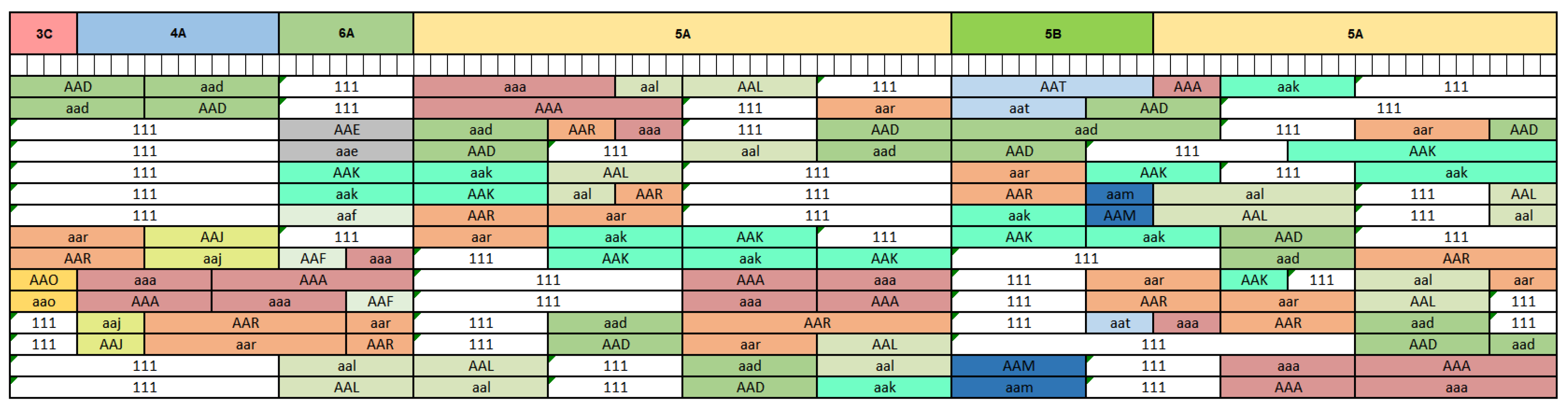
A VNS-based algorithm is run again on the feasible solution output in Phase 2. This algorithm should optimize the objective functions. The objective functions represent the ATCo work and rest periods and positions, ATCo workload distribution, the number of control center changes, and the similarity of the solution structure to the previous template-based solution. The original multi-objective optimization problem is then transformed into a single weighted optimization problem taking into account the objectives ranked by importance by CRIDA experts. This ordinal information is used to specify the centroid-based weights. Solutions are represented by a matrix. The matrix columns represent time slots, and the rows ATCos. Time slots are equivalent to five minutes because five is the greatest common divisor for the applicable constraint times (e.g., ATCos have to work for at least 15 min in the new sector and a sector has to be open for at least 20 min). The Phase 1 heuristic establishes the number of rows, which will not necessarily be the same across the initial solutions.

Each matrix element $(i,j)$ represents the state of ATCo i in time slot j. It is symbolized by three letters. The value 111 represents a resting ATCo, uppercase letters [A-Z] indicate that the ATCo is working as an executive operator, whereas lowercase letters [a-z] are used for planner positions.

Figure 2 illustrates solutions using colors to represent sectors. Rest periods are colored white. Figure 2 shows the solution for the airspace sector configuration illustrated in the Figure 1. This configuration is manned by 15 ATCos (number of rows).

3.1. Phase 1: A Heuristic for the Construction of Initial Solutions

We propose a heuristic to build a set of initial solutions with different rest periods. The Phase 2 algorithm then outputs a feasible solution based on the initial solutions output in Phase 1. The proposed heuristic is based on an optimized template (see Figure 3), with three ATCos covering a sector for 96 time slots (eight hours). ATCo positions (executive or planner) are not assigned until later.

All work periods of are of equal length and twice as long as rest periods. The heuristic builds different, albeit similarly structured, initial solutions if the rest period duration varies. As the working conditions specify that each rest period should last at least 15 min (three slots) and the minimum and maximum work periods are six and twenty four slots, respectively, a rest period must be at least three and at most twelve slots long. Thus, the heuristic builds ten different initial solutions.

The steps of the heuristic are as follows. First, starting from an empty solution, the heuristic adds templates to cover the airspace sectoring. Note that more ATCos than available could be incorporated to the solution in this process. Then, ATCo positions (executive or planner) are allocated taking into account the number of open sectors in each time slot.

Next, we repair the solution to improve feasibility. To do this, we try to transfer a work period without the minimum length from one ATCo to another and extend a work period that does not have the minimum length using a work period from another ATCo.

Finally, we allocate available resources, i.e., we assign an available ATCo to each row in the built initial solution, taking into account the sectors in that row and the ATCo accreditations.

More details about the implementation of the heuristic are available in [10].

3.2. Variable Neighborhood Search and Its Adaptation to the ATC Work-Shift Scheduling Problem

The idea underlying variable neighborhood search (VNS) is to successively explore a set of predefined neighborhoods to find better solutions [11]. VNS explores a set of neighborhoods either at random or systematically in search of local optima. Conducting a local search of diverse neighborhoods potentially generates different local optima, where the global optimum is a local optimum for a given neighborhood. Different neighborhoods generate different landscapes.

The basic version of VNS is shown in Algorithm 1. However, other variants of this basic VNS, such as variable neighborhood descent, reduced variable neighborhood search and variable neighborhood decomposition search can be found in the literature. They depend on:

• The order in which the neighborhoods are used: forward VNS, which starts with $k=1$ and increases k by one if no better solutions are found; otherwise set $k\leftarrow 1$; backward VNS, which starts with $k=k_{max}$ and decreases k by one if no better solutions are found, and extended version, which uses parameters $k_{min}$ and $k_{step}$, sets $k\leftarrow k_{min}$ and increases k by $k_{step}$ if no better solution is found.
• The acceptance of worse solutions. For instance, skewed VNS accepts if $f\left(x^{″}\right)-\alpha d(x,x^{″})<f\left(x\right)$, being $d(x,x^{″})$ the distance between candidate solutions.

Algorithm 1 Basic VNS.

Require: $N_k$: set of neighborhood structures, $k=1,\dots ,k_{max}$ Ensure: Best solution found.   1: $k=1$   2: Generate an initial solution x   3: repeat   4:  Randomly generate $x^{\prime }\in N_k\left(x\right)$   5:  $x^{″}$ = Local-search($x^{\prime }$,$N_k$)   6:  if $(f\left(x^{″}\right)<f\left(x\right))$ then   7:   $x=x^{″}$   8:   $k=1$   9:  else 10:   $k=k+1$ 11:  end if 12: until stopping criterion

The variable neighborhood descent (VND), proposed by [12], changes the neighborhood deterministically. First, the set of neighborhoods and their order are determined, then the algorithm selects an initial solution, and it iterates until it has gone through all the neighborhoods. In each iteration, it performs a search process to reach a local optimum and evaluates if this local optimum is better than the previously derived best solution. If better, it becomes the starting solution for a new local search; otherwise, the algorithm moves on to the next neighborhood to be explored.

The reduced VNS, proposed by [13], is similar to basic VNS except that no iterative improvement procedure is applied. It explores different neighborhoods randomly and quickly reaches good quality solutions for large instances.

The variable neighborhood decomposition search, put forward by [13], generates subproblems by keeping all but k solutions components fixed, and applies local search only to the k ”free” components.

In the biased VNS, reported by [13], once a good solution has been found after a good exploitation, it is usually necessary to move away from this good neighbor to try to find a better solution. This new search is usually very similar to a multi-start heuristic, but this method is usually too expensive in terms of efficiency. Therefore, the algorithm chooses to move towards the best neighbor depending on a distance function between the candidate solutions multiplied by a parametrizable value $\alpha$.

Parallel VNS, described by [14], is a variant aimed at parallelizing the local search processes within VNS to derive and then compare several solutions resulting from starting points.

The VNS adaptation used in this paper is similar to VND in the sense that the algorithm restarts the search process once a solution is found that improves upon the previously best solution. However, whereas VND restarts the process using the same neighborhood definition, our version repeats the search process in all the previously used neighborhood definitions.

Besides, the basic VNS randomly generates a solution from the neighborhood under consideration and starts a local search from this solution, whereas our adaptation of VNS starts the search from the solution in the previous iteration since the local search process is not completely deterministic, rendering the previous step (randomly generate the initial solution) unnecessary.

The following four types of neighborhoods have been considered for the VNS adaptation proposed in this paper:

• First neighborhood. It is based on a time slot exchange between two ATCos fulfilling the following constraints (see Figure 4):

  (a)

  The length of the time interval to be exchanged cannot be greater than 18 slots.

  (b)

  The first ATCo must be located in a row that is higher up than the second ATCo in the solution matrix.

  (c)

  The time interval for the first ATCo must correspond to a work period, whereas, for the second controller, it has to be a rest period.

  (d)

  The exchange process will only be performed if the second ATCo was previously working in the same sector and position just before or after the exchanged time slot (see Figure 4) i.e., we are extending the work period for the second ATCo.

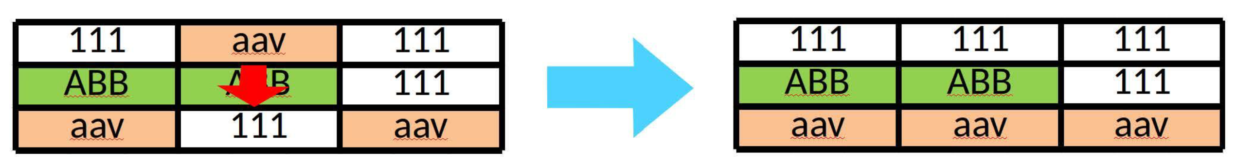
• Second neighborhood. It also consists of a time slot exchange between two ATCos, the only difference from the first neighborhood definition above being that the two time periods involved in the exchange process must be work periods (see Figure 5).
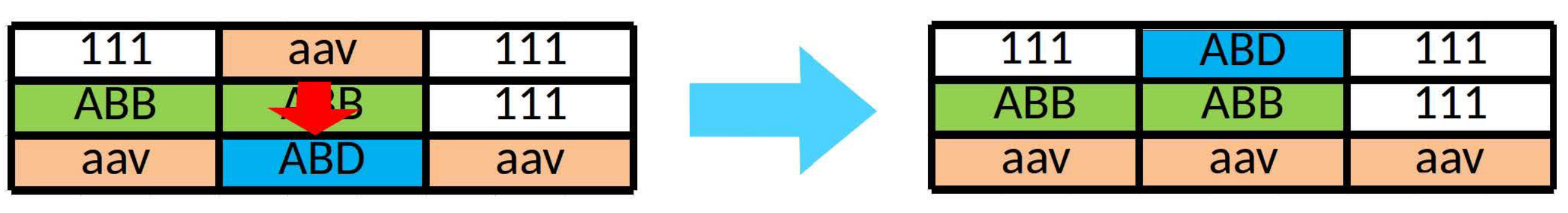
• Third neighborhood. This neighborhood is similar to the first one except for the fact that the exchange process will be performed if the second ATCo was previously working in the same sector and position just before or after the exchange time slot (see Figure 6), i.e., it is not necessary to extend the work period for the second ATCo.
• Fourth neighborhood. This neighborhood is similar to the second one except for the fact that the exchange process will be performed if the second ATCo was previously working in the same sector and position just before or after the exchange time slot (Figure 7), i.e., it is not necessary to extend the work period for the second ATCo.

Figure 8 describes how the four neighborhood definitions are used in our VNS adaptation for Phases 2 and 3, where $time\_int$ represents the time interval length to be exchanged, neighborhood identifies which of the neighborhood definitions under consideration is used, and $laps$ refers to the times number the neighborhood definitions have been used.

The time interval length to be exchanged is initially set to one time slot ($time\_int=1$) and we use the first neighborhood definition ($neighborhood=1$). Then, if the local search outputs a new solution that is better than the current $BestSolution$ in Phase 2, we check if the new solution is feasible. If it is, we output that solution and Phase 2 finishes. If the new solution is not feasible or we are performing Phase 3, then the new solution becomes the $BestSolution$ and a new iteration is carried out.

If the solution achieved in the local search is worse than the current $BestSolution$, the time interval length is increased, and the local search is executed again. If the time interval length is 18 and the output solution is still worse than the current $BestSolution$, then we start using the second neighborhood definition and the time interval length is initialized ($time\_int=1$). If we have used the four neighborhood definitions each with time interval lengths up to 18 and no solutions outperform the current $BestSolution$, then we use the first neighborhood definition again and repeat the process. This process ends when a feasible solution is reached (in Phase 2) or we have used the neighborhood definitions four times ($laps=4$). In the second case, the current $BestSolution$ is the optimal solution.

The local search consists of generating all the possible solutions within the neighborhood with a given time interval ($time\_int$). The generation process is parallelized and the respective solutions are stored in a list in the order in which they are generated. Four seeds are then established to initialize a search process within the list. We use the first seed, which identifies a solution in the list, and randomly move one position to the left or right along the list. If the fitness of the initial solution is not outperformed after exploring 25% of the solutions in the list, then we take the second seed and repeat the process. Once all four seeds have been used, the best solution visited in the process is returned.

Finally, note that we did not consider the same the neighborhood definition as in the SA used by [10] in the VNS adaptation proposed in this paper because the local searches we perform generate all the solutions in the respective neighborhood. This does not pose a problem for the four neighborhood definitions that we use in terms of cardinality. However, the number of solutions in a neighborhood based on the definition used in [10] is very high, which would lead to unaffordable computation times.

3.3. Phase 2: Deriving a Feasible Solution

In Phase 2, VNS is run on an initial solution output in Phase 1. VNS should reduce the number of ATCos covering all open sectors in a given airspace sector configuration to below the available number of ATCos, subject to the ATCo working condition constraints.

The solution matrix output by the Phase 2 search is reordered as follows: the ATCo with the smallest workload is placed at the top, followed by the ATCo with the second smallest workload, and so on. On the other hand, the ATCos with the largest workloads are placed at the bottom. This permutation tends to reduce the number of ATCos as the search progresses.

The fitness function considered in Phase 2 is:

$$maxf=\left\{\begin{array}{c}\hfill w_{1}h+w_{2}g,\mathrm{if}c>n\\ \hfill g,\mathrm{if}c\ge n\end{array}\right.$$

(1)

where c is the number of ATCos for the current solution, n is the number of available ATCos, g is the penalty for all unsatisfied constraints (working conditions) and $w_1$ and $w_2$ represent the relative importance of the components h and g.

Function h should reduce the number of ATCos in the solution below:

$$h=\frac{1}{c^2}\sum _{i=1}^{c}i{h}_i,$$

(2)

where c is the number of ATCos and $h_i$ is the number of work time slots for the i-th ATCo. The term $\frac{1}{c^2}$ means that a decrease in the number of ATCos improves the objective value enormously. Objective values are greater for solutions with a large workload and for ATCos with higher indexes (at the bottom of the solution matrix).

Looking at the objective function and the row permutation of the solutions in Phase 2, the search process appears to reallocate work periods from ATCos at the top of the solution matrix to ATCos in the bottom rows (with the largest workload). This augments the rest periods for the ATCos at the top of the matrix, thus decreasing the number of ATCos required to cover the airspace sector configuration.

Functions h and g must be normalized in order to correctly use the weighted fitness function, see [10].

Note that, in the four neighborhood definitions, condition (b) “The first ATCo must be located in the solution matrix in a row that is higher up than the second ATCo” is considered in the Phase 2 search process only when the number of ATCos in the solutions is greater than the available number of ATCos and is, otherwise, obviated.

Besides, the neighborhoods are initially used in the order in which they were listed in Section 3.2, but numerical experiments prove that the 4-1-3-2 order provides better solutions once the available number of ATCos is reached.

As already mentioned, VNS is conducted starting from an initial solution output in Phase 1. If a feasible solution is not reached in the search process, then we start again with another initial solution output in phase 1 (10 initial solutions were output in Phase 1). The Phase 3 search process starts from the respective feasible solution. This means that Phase 3 is only executed once. Note that a multi-start SA was proposed by [10], in which Phase 2 was executed for the 10 initial solutions derived from Phase 1, and Phase 3 was executed from each feasible solution reached in Phase 2.

3.4. Phase 3: Reaching the Optimal Solution

In Phase 3, VNS is run again, this time on the feasible solution output in Phase 2, in order to optimize the following four objective functions:

• Objective 1: Desirable ATCo work and rest periods, and positions. This objective accounts for three equally important sub-objectives.

  (a)

  The time ATCos remain in the same sector and working position (planner or executive) should be as close as possible to 45 min.

  (b)

  The optimal working time between breaks should be 90 min.

  (c)

  The percentage of ATCo working time in executive positions must be between 40% and 60% of the total working time (not including rest periods).

• Objective 2: Similar solution structure to previous template-based solution. Control center staff will find such a solution easier to understand, and this should facilitate any manual changes. To do this, we analyzed the template-based structure which was used as a benchmark. We concluded that rest and work periods for the same sector should be closely clustered.
• Objective 3: Minimization of the number of control center changes. This objective can be achieved by reducing the number (not the duration) of rest periods.
• Objective 4: Balanced ATCo workloads. ATCo workloads should be balanced in order to avoid high workloads for some, and low workloads for other, ATCs. This is achieved using the standard deviation of the work periods in the different solution matrix rows.

For the mathematical notation and the normalization process of the above objectives and sub-objectives, see [10].

We then transform the original multi-objective optimization problem into a single weighted optimization problem, whose weights, $w_i$, are derived using the rank-order centroid (ROC) method [15]. This single weighted optimization accounts for the ordinal information provided by CRIDA experts.

Finally, note that, in the four neighborhood definitions, condition (b) “The first ATCo must be located in the solution matrix in a row that is higher up than for the second ATCo” is not considered in the Phase 3 search process. Moreover, numerical experiments prove that the 2-1-3-4 neighborhood order provides better solutions. Note also that the infeasible solutions generated using the corresponding neighborhood definition in the Phase 3 local searches are not stored in the list.

4. Results: VNS and SA Performance Analysis

In this section, we illustrate the proposed methodology and compare the performance of VNS against SA in Phases 2 and 3 on the basis of four representative and complex instances of the problem corresponding to different airspace sectorings selected by CRIDA experts.

4.1. Illustrative Instances

Instance 1. Morning shift in Barcelona control center (10 different open sectors). Figure 9 shows the airspace sectoring of the Barcelona control center. It consists of a morning shift covering from 5:20 to 13:00 with 10 different open sectors:

• 3 open sectors (LECBLEGL, LECBLGU, LECBPPI) from 5:20 to 6:00,
• 4 open sectors (LECBLEGL, LECBLGU, LECBP1I, LECBPP2) from 6:00 to 7:40,
• 5 open sectors (LECBP1I, LECBPP2, LECBLVL, LECBLVS, LECBLVU) from 7:40 to 8:40,
• 6 open sectors (LECBPP2, LECBLVL, LECBLVS, LECBLVU, LECBP1L, LECBP1U) from 8:40 to 12:00, and
• 5 (LECBP1I, LECBPP2, LECBLVL, LECBLVS, LECBLVU) from 12:00 to 13:00. All the sectors and controllers involved belong to the western route core. The number of available controllers is 16, and their accreditation type is CON.

The problem posed by this instance is the percentage resting time constraint, where all ATCos must rest for 25% of the shift. If 16 ATCos cover 6 sectors (two templates of 3 sectors with 8 ATCos, which is optimized), the ATCos must work exactly 75% of the time. This implies that the work distribution slack is zero, and the working time for all ATCos is exactly equal, whereas all other constraints are met.

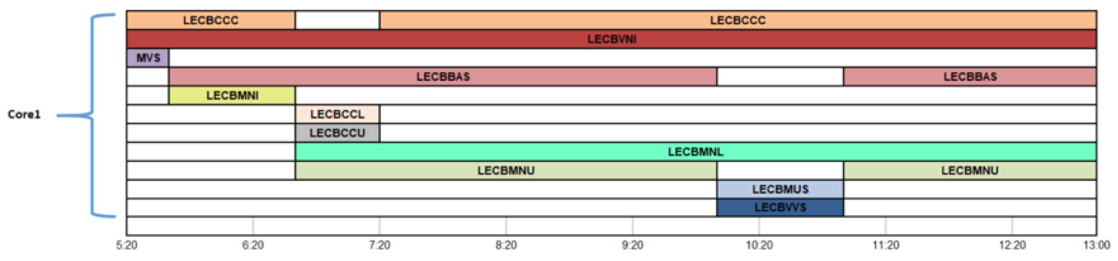
Instance 2. Morning shift in Barcelona control center (11 open sectors).Figure 10 shows the airspace sectoring of the Madrid control center. It consists of a morning shift, which covers from 5:20 to 13:00 with 11 open sectors: 3 open sectors from 5:20 to 8:40, 4 open sectors from 5:40 to 6:40, 6 open sectors from 6:40 to 7:20, 5 open sectors from 7:20 to 10:00, 5 open sectors from 10:00 to 11:00, and from 11:00 to 13:00. All the sectors and ATCos involved belong to the eastern route core. There are 15 available ATCos, whom are CON accredited.

The problem posed by this instance is sector opening and closing. We must also cover 6 sectors opened for 40 min with only 15 controllers. Note that an additional ATCo would be necessary if these sectors were to remain open for longer.

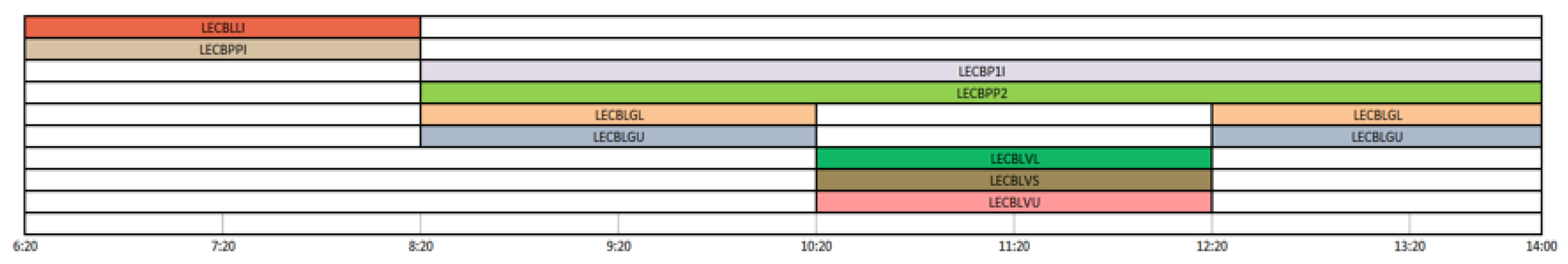
Instance 3. Morning shift in Barcelona control center (9 open sectors).Figure 11 shows the airspace sectoring of the Barcelona control center for a morning shift, covering from 6:20 to 14:00 with 9 sectors open: 2 open sectors from 6:20 to 8:20, 4 sectors open from 8:20 to 10:20, 5 sectors open from 10:20 to 12:20, and 4, from 12:20 to 14:00. All the sectors and ATCos involved belong to the eastern route core. There are 14 available ATCos, all whom hold CON accreditation.

It is a relatively simple example, but there are quite a few changes of sectors that complicate the fulfillment of all constraints.

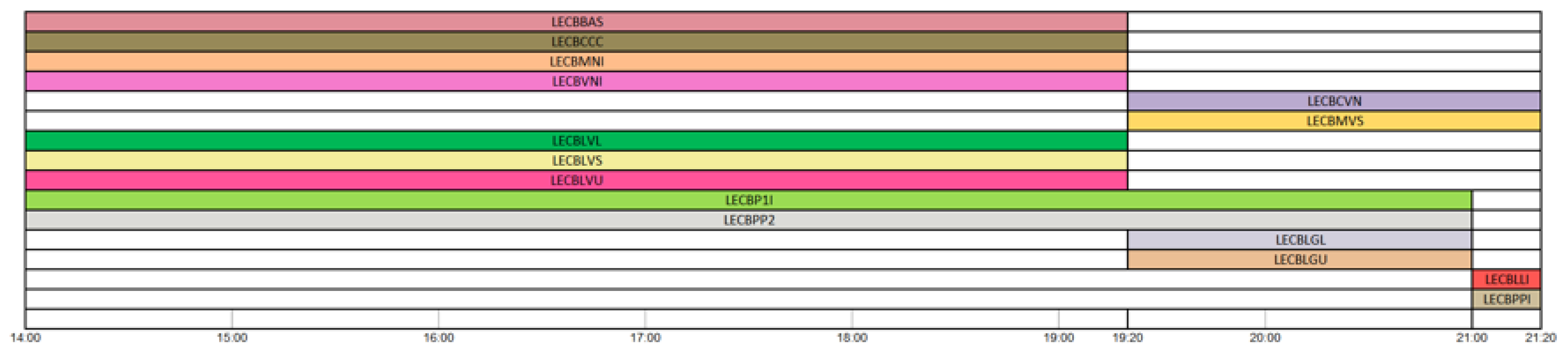
Instance 4. Afternoon shift in Barcelona control center (6 open sectors).Figure 12 shows the airspace sectoring of the Barcelona control center for an afternoon shift, covering from 14:00 to 21:20. There are 6 open sectors in the Barcelona western route core: 4 sectors open from 14:00 to 19:20, and 2 sectors open from 19:20 to 21:20; and 9 sectors open in the Barcelona eastern route core: 5 sectors open from 14:00 to 19:20, 4 sectors open from 19:20 to 21:00, and 2 sectors open from 21:00 to 21:20. The number of available ATCos is 28, whose accreditation type is CON, 14 belonging to the eastern and 14 to the western core.

The main problem posed by this instance is its size. A large number of ATCos are needed to cover all sectors. In addition, there is a progressive closure of sectors, where ATCos are highly unlikely to comply with the minimum consecutive work constraint, among others.

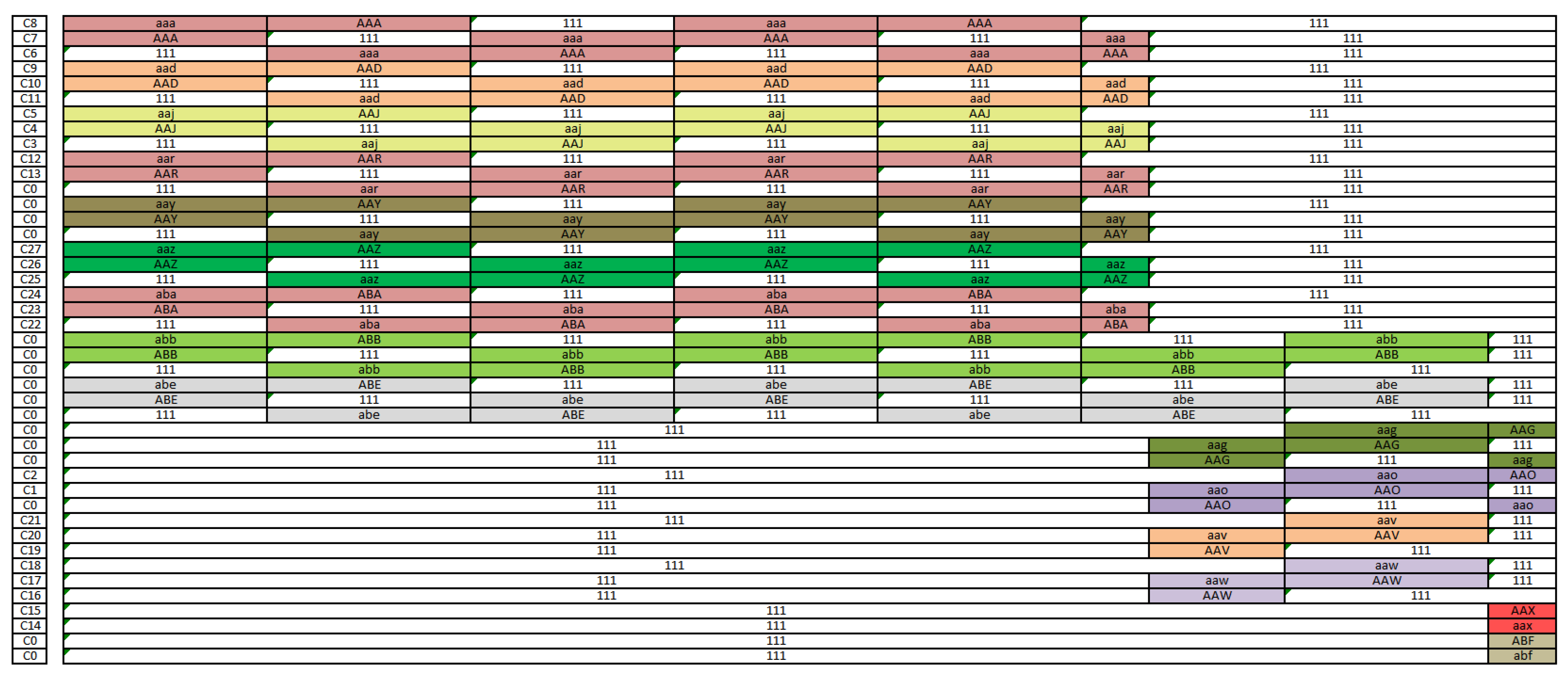
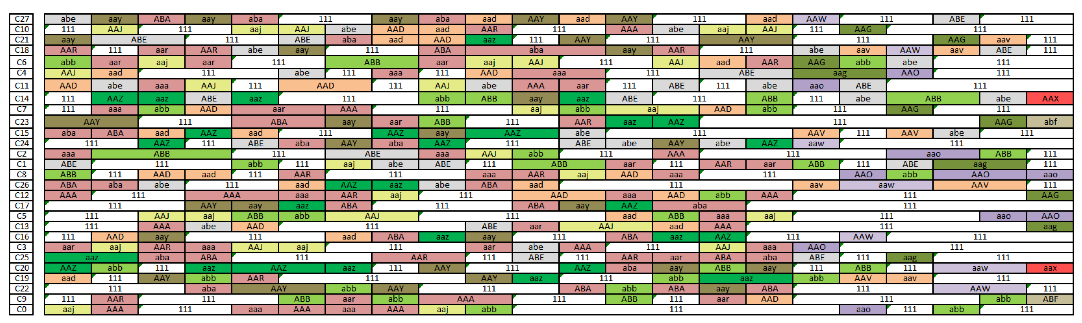
Figure 13, Figure 14 and Figure 15 illustrate an initial solution of this last instance, the corresponding feasible solution and the optimal solution reached using VNS in Phases 2 and 3, respectively. Looking at Figure 13, we find that optimized templates are used where three ATCos cover a sector for 96 time slots and the number of necessary ATCos (43) is greater than the number that are actually available ATCos (28). 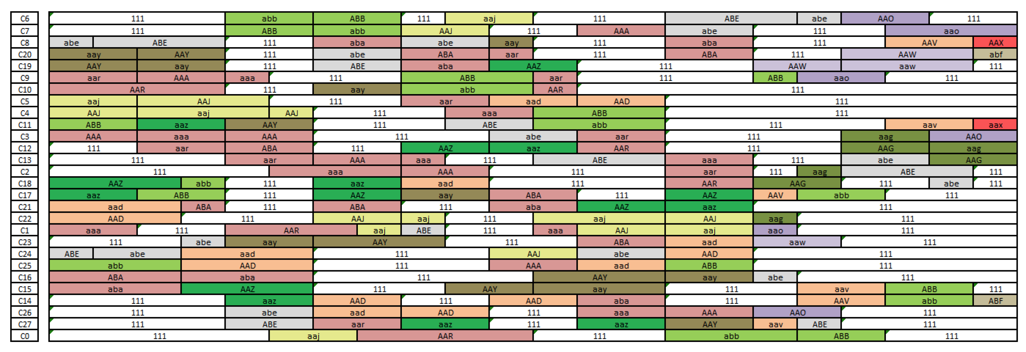Figure 14 shows the feasible solution derived from Phase 2 using VNS. Now the number of ATCos matches 28, and all labor conditions are met. Finally, Figure 15 shows the optimal solution derived in Phase 3 using VNS. If we compare the initial feasible and the optimal solutions, it is clear that the structure of the optimal solution is like the previous template-based solution, where work and rest periods are more concentrated.

Table 1. Objective functions in the initial and optimal solution in Instance 4.

	ATCo Work and Rest Periods and Positions			Objective 3	ATCo Workloads
	Sub-Object. 1	Sub-Object. 2	Sub-Object. 3	Rest Periods	$\mathit{\sigma }$	min	max
Initial	$27.9,44.9,71.7\%$	$24.4,24.4,38.3\%$	$81.3,85.4,86.4\%$	122	87.3	17	293.5
VNS	$9.37,11.45,23.95\%$	$10.12,12.65,14.55\%$	$95,98,100\%$	160	58.13	115	330

shows three out of the four original objectives, optimizing the ATCo work and rest periods and positions, the number of control center changes (rest periods), and the distribution of the ATCo workload.

The first column (sub-object. 1) shows the percentage of cases with a difference less than or equal to 10, 15 and 25 min, respectively, with respect to the goal of 45 min. The second column (sub-object. 2) shows the percentage of cases with a difference less than or equal to 15, 20 and 25 min, respectively, with respect to the goal of 90 min. The third column (sub-object. 1) shows the ATCo percentages whose differences are lower than or equal to 5%, 10% and 15%, respectively. The fourth column shows the number of rest periods, and, finally, the fifth column (ATCo workloads) lists the standard deviation, and the minimum and the maximum value of the ATCo workloads.

As expected, the optimal solution outperforms the initial one for all the objectives under consideration.

4.2. Computational Improvements

All the constraints with respect to the ATCo labor conditions must be checked to verify the feasibility of the analyzed solutions in the different iterations of the VNS execution. In Phase 2, this constraint verification is associated with the fitness function, since this phase is aimed at reaching a feasible solution, whereas the Phase 3 search process is carried out within the feasible region, on which ground we have to check the feasibility of the visited solutions.

Verifying constraints is very time consuming. Therefore, we have carried out a comparative analysis to check if this process is faster using regular expressions, which, apart from structuring the constraint modularly could lead to better computation times than implementing such constraints in the code.

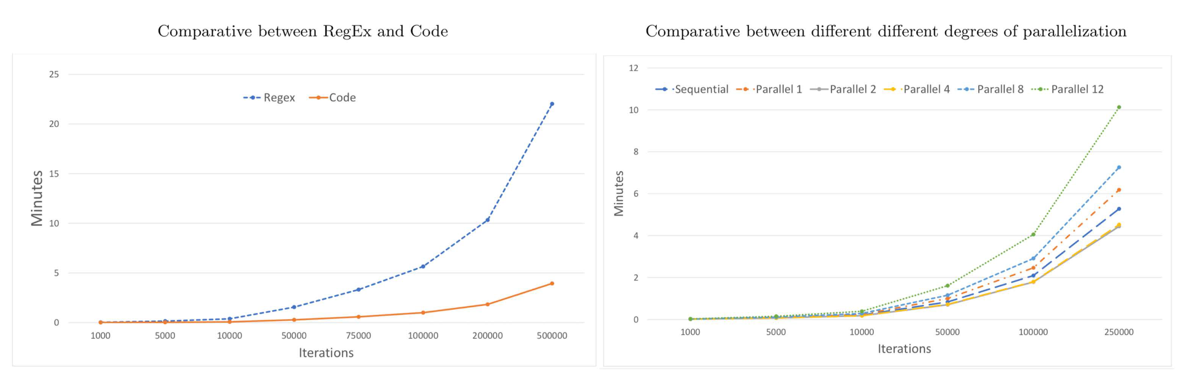
Figure 16 shows the mean execution times throughout the iterations in the proposed VNS adaptation using both regular expressions and the code implementation for Instance 4. Contrary to what we had initially thought, the code implementation outperforms the use of regular expressions for higher numbers of iterations. This is due to the complexity of some of the constraints to be checked, requiring lot more than one number of regular expression.

Additionally, the parallelization of the constraint verification process could improve computation times. Figure 16 shows the different execution times with and without different degrees of parallelization (up to 12 simultaneous threads), again for Instance 4. As expected, parallelization offers faster speeds with respect to sequential execution. We find that there are significant improvements as the number of threads increases, up to four threads.

These results are logical taking into account the computer that we used, which had a quad-core processor. Therefore, it works better when the number of threads used in the execution is also four. When more than four threads are used, they all share the CPU time and sometimes have to wait in a queue to be processed. These CPU inputs and outputs are time consuming and make the process less efficient. However, a CPU with a higher number of cores would take better advantage of more parallelized threads.

Similar results were output for the other three instances.

5. Discussion

In this section, we compare the performance of VNS against the multi-start SA used by [10] for the four complex instances under consideration, taking into account both the quality of the solution reached by means of the fitness function and the four original objectives and execution times.

Each instance was executed 10 times using a Intel(R) Xeon(R) E3-1240 PC with 3.50 GHz and 16 GB of RAM, running Windows 10.

Table 2. Optimal fitness values in Phase 3 for SA and VNS.

	SA			VNS
	Min	Mean	Max	Min	Mean	Max
Inst. 1	0.8637	0.8689	0.875	0.853	0.857	0.863
Inst. 2	0.8714	0.8742	0.8769	0.845	0.853	0.858
Inst. 3	0.8915	0.8946	0.8968	0.876	0.887	0.896
Inst. 4	0.8527	0.8604	0.867	0.854	0.855	0.856

shows the minimum, mean and maximum values of the fitness function in the optimal solutions achieved by the VNS and SA. The mean values for SA are clearly higher than for VNS in all four instances under consideration. We can thus conclude that SA slightly outperforms VNS with respect to the quality of the solutions reached.

Let us analyze in depth the optimal solutions derived by both metaheuristics in the four instances under consideration.

Table 3. Objective functions in the initial solution and solutions reached by SA and VNS for Instance 1.

	ATC Work and Rest Periods and Positions			Obj. 2	Obj. 3	ATCo Workloads
	Sub-Object. 1	Sub-Object. 2	Sub-Object. 3	Similarity	Rest Periods	$\mathit{\sigma }$	Min	Max
Initial	$26.7,41.2,70.8$	$18.2,20.9,30.8$	$87.3,94.2,94.5$	81.9	51.2	67.1	35	292.5
SA	$35.6,35.6,85.6$	$\mathbf{31.4},\mathbf{66.6},\mathbf{66.6}$	100,100,100	$71.77$	51	20.45	255	325
VNS	$\mathbf{47.9},\mathbf{52},\mathbf{86.7}$	$25.9,61.1,61.1$	100,100,100	$68.7$	54	25.4	240	330

,

Table 4. Objective functions in the initial solution and solutions reached by SA and VNS for Instance 2.

	ATC Work and Rest Periods and Positions			Obj. 2	Obj. 3	ATCo Workloads
	Sub-Object. 1	Sub-Object. 2	Sub-Object. 3	Similarity	Rest Periods	$\mathit{\sigma }$	Min	Max
Initial	$24.3,38,62.5$	$16.4,17.1,25.4$	$61.9,66.7,67.3$	75.6	59.3	116.6	15	319.5
SA	$\mathbf{65.2},\mathbf{65.2},80$	$\mathbf{38.3},38.3,38.3$	100,100,100	$74.88$	46	18.5	280	340
VNS	$50,63.1,\mathbf{86.8}$	$30.9,\mathbf{41.8},\mathbf{45.4}$	100,100,100	71	54	16.3	275	330

,

Table 5. Objective functions in the initial solution and solutions reached by SA and VNS for Instance 3.

	ATC Work and Rest Periods and Positions			Obj. 2	Obj. 3	ATCo Workloads
	Sub-Object. 1	Sub-Object. 2	Sub-Object. 3	Similarity	Rest Periods	$\mathit{\sigma }$	Min	Max
Initial	$25.3,38.1,67.6$	$16.5,19.2,25.2$	$85.1,90.4,94.1$	84.7	43.5	60.8	70	238.5
SA	$\mathbf{75},\mathbf{75},88.1$	$30.1,30.1,30.1$	100,100,100	$80.55$	38	34.9	220	320
VNS	$54.6,63.9,\mathbf{91.8}$	$\mathbf{32.4},\mathbf{40},\mathbf{47.5}$	100,100,100	$79.6$	42	21.2	210	280

and

Table 6. Objective functions in the initial solution and solutions reached by SA and VNS for Instance 4.

	ATC Work and Rest Periods and Positions			Obj. 2	Obj. 3	ATCo Workloads
	Sub-Object. 1	Sub-Object. 2	Sub-Object. 3	Similarity	Rest Periods	$\mathit{\sigma }$	Min	Max
Initial	$27.9,44.9,71.7$	$24.4,24.4,38.3$	$81.3,85.4,86.4$	67.6	122	87.3	17	293.5
SA	$56.6,56.6,76.6$	$40,40,40$	100,100,100	$\mathbf{73.05}$	77	32	$\mathbf{200}$	320
VNS	$\mathbf{64.7},\mathbf{74.6},\mathbf{90}$	$\mathbf{41.2},\mathbf{53.9},\mathbf{58.8}$	84,88.7,88.7	$68.6$	193	19.2	212.5	290

show the values of the initial solution and solutions reached by VNS and SA for the four instances under consideration, respectively, in terms of the four original objectives, optimizing the ATCo work and rest periods and positions, the similarity to the previous template-based solution, the number of control center changes (rest periods), and the distribution of the ATCo workload.

Note that Table 3, Table 4, Table 5 and Table 6 provide mean values, and the respective best values for each column are highlighted in bold.

Looking at sub-object. 1, we find that VNS outperforms SA for 8 out the 12 mean values shown in Table 3, Table 4, Table 5 and Table 6; whereas SA is better than VS for sub-object. 2 in the first instance but not for instances 3 and 4.

As expected, the initial solution outperforms the solutions reached by SA and VNS in terms of similarity to previous template-based solution. However, SA outperforms VNS with respect to this objective in all four instances under consideration.

Regarding the number of rest periods, SA outperforms VNS for all four instances under consideration. For all four instances, the number of rest periods in VNS is [10.67, 17]% higher than for SA.

Finally, looking at the standard deviation representing the ATCo workload dispersion, we find that SA outperforms VNS for the first instance, whereas VNS is better for Instances 2, 3 and 4. In all four cases, the ATCo workload dispersions were very similar in both metaheuristics.

These tables were shown to CRIDA experts, who analyzed the quality of the solutions reached by VNS and SA for the four complex instances. They concluded that, although the solutions derived by SA slightly outperform those reached using VNS in terms of the fitness function, the quality of both solutions were very similar four the four instances under consideration and that the key factor was then the time it took to reach that solutions, i.e., the computation times.

Table 7. Computation times (in minutes) in Phase 2.

	Original SA			Improved SA			VNS
	Min	Mean	Max	Min	Mean	Max	Min	Mean	Max
Instance 1	206.21	254.71	333.24	5.79	6.02	6.25	8.73	9.26	10.15
Instance 2	207.34	249.59	308.14	16.34	17.64	19.76	4.28	7.14	11.29
Instance 3	111.7	128.96	157.88	3.64	6.75	12.92	4.11	4.65	5.50
Instance 4	394.69	507.25	619.82	48.88	49.53	50.48	100.71	111.85	122.18

and

Table 8. Computation times (in minutes) in Phase 3.

	Original SA			Improved SA			VNS
	Min	Mean	Max	Min	Mean	Max	Min	Mean	Max
Instance 1	177.59	214.76	262.47	40.52	54.04	68.54	21.48	31.12	43.84
Instance 2	79.87	95.19	122.37	27.52	36.89	50.47	28.55	30.68	33.08-
Instance 3	103.19	139.24	210.34	24.67	25.33	26.46	16.01	19.75	24.68
Instance 4	802.16	958.25	1114.35	177.25	247.87	360.72	431.15	479.66	507.79

show the minimum, mean and maximum computation times (in minutes) in Phases 2 and 3, respectively, for the original multi-start SA proposed by [10], an improved non multi-start SA using a constraint implementation in the code rather than regular expressions and with parallelization (4 threads), and the proposed adaptation of VNS (also using a constraint implementation in the code and with parallelization). The metaheuristic with the lowest computation time is highlighted in bold.

The first thing that we found is that the computation times for the improved SA are much lower than for the original SA in both phases and for the four instances under consideration, as was expected. Besides, computation times for Phase 3 are quite a lot higher than in Phase 2, accounting for the biggest share of the accumulated computation times shown in

Table 9. Mean accumulated computation times (in minutes).

	Original SA	Improved SA	VNS
Instance 1	469.49	60.09	40.38
Instance 2	344.79	54.54	37.81
Instance 3	268.21	32.1	24.40
Instance 4	1465.52	297.43	591.52

.

If we focus on Phase 2, VNS and SA outperform each other in two out of the four instances. However, although the mean computation times for Instances 1 and 3 are similar, VNS clearly outperforms SA in Instance 2, whereas the opposite applies for Instance 4 (SA is more than 70 min faster than VNS). Note that Instance 4 involves a larger number of open sectors and required ATCos.

In Phase 3, VNS clearly outperforms SA in instance 1 but it is only slightly better for Instances 2 and 3. In Instance 4, SA clearly outperforms VNS with a difference of close to 200 min in the mean computation times.

Looking at the mean accumulated computation times in Table 9, we find that VNS clearly outperforms SA in Instances 1 and 2, they are similar for Instance 3, but SA is quite a lot better in Instance 4.

We have analyzed other sectorizations provided by CRIDA in order to verify whether or not the performance of VNS is sensitive to the instance dimension, as in the case of Instance 4, and we have confirmed this hypothesis: the improved SA outperforms VNS when the dimensionality (number of open sectors and required ATCos) is high in all cases, whereas VNS is clearly better in any other situation with a low and medium number of dimensions.

Note that although the mean computation time accumulated in Instance 4 is about 5 h (297.43 min) with the improved SA, which could be considered a high computation time, the complexity of this instance is the highest (9 simultaneously open sectors and 28 ATCos) that could materialize in Spanish airports. Consequently, the maximum computation time of this instance, $50.58$ min + $360.72$ min $\simeq 7$ h could be considered, as an upper bound for the computation times. In most cases, solutions are reached in the less than an hour.

Taking into account that the pre-tactical phase takes place one to six days before the day of operations, the CRIDA experts considered this a good upper bound for computation times.

6. Conclusions

We have proposed a new methodology based on an adaptation of VNS for solving the ATCo work-shift scheduling problem. This problem involves covering a given airspace sectoring with a certain number of ATCos while satisfying a set of ATCo labor conditions according to Spanish regulations. The problem takes into account four objectives: ATCo work and rest periods and position should be as close as possible to fixed values, the solution structure should be similar to the previous template-based solution, the number of control center changes should be minimized, and the ATCo workload distribution should be balanced.

A comparative analysis proves that the constraint verification in search processes is faster with the implementation in the code of such constraints than using regular expressions. Besides, the parallelization of the constraint verification process has also been analyzed in terms of computation times.

Finally, the proposed methodology has been applied to four real complex scenarios selected by Spanish air navigation experts for the purposes of both methodology illustration and performance comparison against two versions of simulated annealing (SA).

Although the SA-derived solutions slightly outperform VNS solutions in terms of the fitness function, air navigation experts regard the quality of both solutions as very similar, where the key factor then is the time it takes to reach that solutions (computation times). VNS clearly outperforms SA in terms of computation times when the instance dimension (number of open sectors and ATCos required) is low or medium, but the improved version of SA is better for high dimensional instances.

Finally, although the CRIDA experts considered than the computation times for the most complex instances, such as instance 4, were good enough for the pre-tactical phase, which takes place one to six days before the day of operations, we propose as a future research line a further analysis to reduce these computation times together with the comparison of the considered metaheuristics with other in the literature.