A Fast Derivative-Free Iteration Scheme for Nonlinear Systems and Integral Equations

Abstract

Derivative-free schemes are a class of competitive methods since they are one remedy in cases at which the computation of the Jacobian or higher order derivatives of multi-dimensional functions is difficult. This article studies a variant of Steffensen’s method with memory for tackling a nonlinear system of equations, to not only be independent of the Jacobian calculation but also to improve the computational efficiency. The analytical parts of the work are supported by several tests, including an application in mixed integral equations.

1. Introductory Notes

1.1. Background

There exist many works handling the approximate solution of linear and nonlinear integral equations. However, tackling nonlinear integral equations would be more challenging due to the presence of nonlinearity which might be expensive for different solvers [1,2].

Some authors discussed the asymptotic error expansion of collocation-type and Nystrom-type methods for Volterra–Fredholm integral equations with nonlinearity, see [3] for a complete discussion on this issue. One class of nonlinear internal equations is the mixed Hammerstein integral equations with several application in engineering problems [2].

Since in the process of finding the solution of such integral equations, most of the time a system of algebraic equation would occur that must be solved quickly and accurately, thus we here bring the attention to develop and study a useful numerical solution scheme for solving nonlinear systems with application in tackling nonlinear integral equations.

Clearly, there are some other nonlinear problems in literature which could yield in tackling nonlinear system of equations, see e.g., [4,5].

1.2. Definition

Consider a nonlinear system of equations of algebraic type as follows [6]:

$$\left\{\begin{array}{c}{a}_1(x_1,x_2,\dots ,x_m)=0,\hfill \\ a_2(x_1,x_2,\dots ,x_m)=0,\hfill \\ ⋮\hfill \\ a_m(x_1,x_2,\dots ,x_m)=0,\hfill \end{array}\right.$$

(1)

which contains m equations with m unknowns and $A(x)$ $={(a_1(x),a_2(x),\dots ,a_m(x))}^T$ while $a_1(x)$, $a_2(x)$, …, $a_m(x)$ are the functions of coordinate. We can also write (1) using $x=(x_1,x_2,\dots ,x_m)$ in a more compact form as

$$A(x)=0.$$

(2)

The purpose of this work is to study finding the solution of system (1) via iteration process and discuss its application in solving nonlinear integral equations. As such, now let us briefly review some of the existing methods for finding its simple roots in the next subsection.

1.3. Existing Solvers

The Steffensen’s scheme for solving nonlinear systems is written as follows [7]:

$$\left\{\begin{array}{c}{w}^{(n)}=x^{(n)}+A(x^{(n)}),x^{(0)}\in {\mathbb{R}}^m,\hfill \\ x^{(n+1)}=x^{(n)}-{[x^{(n)},w^{(n)};A]}^{-1}A(x^{(n)}),n=0,1,2,\cdots ,\hfill \end{array}\right.$$

(3)

which is based upon the divided difference operator (DDO). The 1st order DDO of A for the multidimensional nodes x and y is expressed by a component-to-component procedure as follows [8]:

$${[x,y;A]}_{i,j}=\frac{A_i(x_1,\dots ,x_j,y_{j+1},\dots ,y_m)-A_i(x_1,\dots ,x_{j-1},y_j,\dots ,y_m)}{x_j-y_j},1\le i,j\le m.$$

(4)

Recall that first-order divided difference of A on ${\mathbb{R}}^m$ is a mapping as follows:

$$[·,·;A]:D\subset {\mathbb{R}}^m\times {\mathbb{R}}^m\to \mathcal{L}({\mathbb{R}}^m),$$

(5)

that reads

$$[y,x;A](y-x)=A(y)-A(x),\forall x,y\in D.$$

(6)

Here $\mathcal{L}(·)$ shows the set of bounded linear functions. By considering $h=y-x$, one we can also express the first-order DDO as follows [8]:

$$\left[x+h,x;A\right]={\int }_0^1{A}^{\prime }(x+th)dt,\forall (x,h)\in {\mathbb{R}}^m\times {\mathbb{R}}^m.$$

(7)

Traub in [9] investigated another way based on the function $J(x,H)$ for approximating the Jacobian matrix of the Newton’s method and to obtain the Steffensen’s scheme based on a point-wise definition.

An improvement of (3) was given in [10,11] as follows:

$$\left\{\begin{array}{c}{z}^{(n)}=x^{(n)}-{[x^{(n)},w^{(n)};A]}^{-1}A(x^{(n)}),\hfill \\ x^{(n+1)}=z^{(n)}-{[x^{(n)},w^{(n)};A]}^{-1}A(z^{(n)}),\hfill \end{array}\right.$$

(8)

wherein

$$w^{(n)}=x^{(n)}+\beta A(x^{(n)}),\beta \in \mathbb{R}.$$

(9)

The point in (8) in contrast to (3) is that it applies two steps and of course two m-D functional evaluations to reach a higher rate than quadratic. Here, the idea is to freeze the DDO per cycle and then increase the sub steps so as to gain as much as possible of order improvement, as well as some improvements in the computational efficiency index of the scheme.

Let us also recall some of the iteration schemes having the requirement of Jacobian computation now. The Jarratt’s iteration having fourth rate of convergence for solving (1) is given by [12]:

$$\left\{\begin{array}{c}{z}^{(n)}=x^{(n)}-\frac{2}{3}{A}^{\prime }{(x^{(n)})}^{-1}A(x^{(n)}),\hfill \\ x^{(n+1)}=x^{(n)}-\frac{1}{2}{(3A^{\prime }(z^{(n)})-A^{\prime }(x^{(n)}))}^{-1}\hfill \\ \times (3A^{\prime }(z^{(n)})+A^{\prime }(x^{(n)}))A^{\prime }{(x^{(n)})}^{-1}A(x^{(n)}).\hfill \end{array}\right.$$

(10)

This fourth-order iteration expression requires the computation of two matrix inverses (based on the resolution of linear systems) to achieve its rate, which manifest that getting higher rate of convergence in the form of a two-step method is costly.

1.4. Motivation

All methods discussed until now are without memory; some improvements over such schemes can be done by considering additional memory terms.

Our motivation of pursuing this aim is not only limited at tackling nonlinear systems, but a motivation is to apply such schemes for practical engineering problems such as the nonlinear mixed integral equations, see e.g., [13,14,15,16].

The goal in our development is to reach a higher computational efficiency using as low as possible number of linear systems of equations and the functional evaluations. This is directly interlinked with the concept of scientific computing and numerical analysis which gives a meaning to the investigation and proposing novel numerical procedures.

1.5. Achievement and Contribution

The objective of this work is to present a two-step higher order scheme to solve system of nonlinear equations. As such, we present an iteration method with memory for finding both real and complex zeros. Our scheme does not require computing the Fréchet derivatives of the function.

1.6. Organization

We unfold this article as follows. In Section 2, the derivation and contribution of an iteration expression is furnished. Section 3 provides an error analysis for its convergence rate. The computational efficiency of different solvers by including not only the number of functional evaluations, but also the number of system of involved linear equations, the number of LU (Lower-Upper) factorizations as well as the other similar operations will be discussed in Section 4 in detail. Section 5 discusses the application of the proposed scheme. Concluding remarks are given in Section 6.

2. A Derivative-Free Scheme

Here our attempt is to increase the computational efficiency index of (8) without imposing several more steps or further DDDs in each cycle. To complete such a task, we rely on the concept of methods with memory which state that the convergence speed and efficiency of iterative methods could be improved by saving and using the already computed values of the functions and nodes.

In fact, the error equation of the uni-parametric family of methods (8) includes a term of the form below:

$$I+\beta A^{\prime }(\alpha )=0.$$

(11)

The free nonzero parameter $\beta$ in (11) can clearly affect not only on the domain of convergence (attraction basins of the iterative method) but also to the improvement of the convergence order. When tackling a nonlinear system of equations, and since $\alpha$ is not known, we can use an approximation for $A^{\prime }(\alpha )$ to make the whole relation (11) approximately zero. Therefore, we may write

$$\beta \simeq -A^{\prime }{(\overline{\alpha })}^{-1},$$

(12)

wherein $\overline{\alpha }$ is an approximation of the solution (per cycle).

It is important to discuss how we approximate the matrix $\beta :=B^{(n)}(n\ge 1)$ by employing some estimates to $-A^{\prime }(\alpha )$ computed via the existing data.

To improve the performance of (8) using the notion of methods with memory, we consider the following iteration expression:

$$\left\{\begin{array}{cc}\hfill w^{(n)}& =x^{(n)}+\beta A(x^{(n)})\hfill \\ \hfill z^{(n)}& =x^{(n)}-{[x^{(n)},w^{(n)};A]}^{-1}A(x^{(n)}),\hfill \\ \hfill x^{(n+1)}& =z^{(n)}-{[x^{(n)},w^{(n)};A]}^{-1}A(z^{(n)}).\hfill \end{array}\right.$$

(13)

To ease up the implementation of the scheme with memory, let us first consider

$$\beta :=B^{(n)}=-{[w^{(n-1)},x^{(n-1)};A]}^{-1}=-{M^{(n-1)}}^{-1}\approx -A^{\prime }{(\alpha )}^{-1}.$$

(14)

and

$$\left\{\begin{array}{c}{M}^{(n-1)}{\delta }^{(n)}=A(x^{(n)}),\hfill \\ M^{(n-1)}{\gamma }^{(n)}=A(y^{(n)}).\hfill \end{array}\right.$$

(15)

Thus, now we contribute the following scheme:

$$\left\{\begin{array}{c}{B}^{(n)}=-{[w^{(n-1)},x^{(n-1)};A]}^{-1},n\ge 1,\hfill \\ w^{(n)}=x^{(n)}+B^{(n)}A(x^{(n)}),n\ge 1,\hfill \\ y^{(n)}=x^{(n)}+{\delta }^{(n)},n\ge 0,\hfill \\ x^{(n+1)}=y^{(n)}+{\gamma }^{(n)}.\hfill \end{array}\right.$$

(16)

Lemma 1.

Let $D\subset {\mathbb{R}}^m$ be a nonempty convex domain. Suppose that A is thrice Fréchet differentiable on D, and that $[u,v;A]\in \mathcal{L}(D,D)$, for any $u,v\in D(u\ne v)$ and the initial value $x^{(0)}$ and the solution α are close to each other. By considering $B^{(n)}$ = $-{[w^{(n-1)},x^{(n-1)};A]}^{-1}$ and $d^{(n)}:=I+B^{(n)}{A}^{\prime }(\alpha )$, one obtains the error relation below

$$d^{(n)}\sim e^{(n-1)}.$$

(17)

Proof. 

See [17] for more details.  ☐

To implement (16), one needs to solve some linear systems of algebraic equations. This means that at each new step, a new LU factorization is needed, and no information can be exploited from the previous steps. However, there exists a body of literature about recycling this kind of information to obtain updated preconditioner for iterative solvers, [18,19,20]. We leave future discussion about constructing and imposing such a preconditioner for future works in this field.

As long as the coefficient matrices are sparse or large and sparse, a Krylov subspace method can be employed to speed up the process. However, the merit in (16) is that the two linear systems have one same coefficient matrix. Hence, only one LU factorization would be enough and by saving the decomposition, one can act it to two different right-hand-side vectors to get the solution vectors per sub cycles of (16).

A challenging part of the implementation using (16) is the incorporation of $B^{(n)}$. This is a not anymore a constant and it should be defined as a matrix. In this paper, whenever required the initial matrix $B^{(0)}$ is specified by:

$${B^{(0)}}^{-1}=\mathrm{diag}\left(-\frac{1}{1000}\right).$$

(18)

The choice of the initial matrix $B^{(0)}$ affects directly on the whole process in order to arrive in the convergence phase as quickly as possible. Here, (18) is in agreement with the dynamical studies of Steffensen-type methods with memory at which the basins of attractions are larger as long as the free parameter is close to zero.

Noting also that updating $B^{(n)}$ per cycle is again based on the already computed LU factorization while it should only act on the identity matrix to proceed.

3. Rate of Convergence

It is known that via the Taylor expansion of $A^{\prime }(x+th)$ in the node x and integrating, one obtains:

$${\int }_0^1{A}^{\prime }(x+th)dt=A^{\prime }(x)+\frac{1}{2}{A}^{″}(x)h+\frac{1}{6}{A}^{‴}(x)h^2+\frac{1}{24}{A}^{(iv)}(x)h^3+\mathcal{O}(h^4).$$

(19)

It is here assumed that $A^{\prime }(\alpha )$ is not singular and $e^{(n)}=x^{(n)}-\alpha$ is called the error at the n-th iterate and [6,21]:

$$e^{(n+1)}=H{e}^{{(n)}^p}+\mathcal{O}(e^{{(n)}^{p+1}}),$$

(20)

(20) is the equation of error, whereas H is a p-linear function. This means that $H\in \mathcal{L}({\mathbb{R}}^m,{\mathbb{R}}^m,\dots ,{\mathbb{R}}^m)$. Moreover, we consider:

$$e^{{(n)}^p}=(\underset{p\mathrm{times}}{\underbrace{e^{(n)},e^{(n)},\dots ,e^{(n)}}}),$$

(21)

which would be a matrix.

Before stating the main theorem, it is pointed out that if A be differentiable in terms of Fréchet concept in D sufficiently. As in [22], the l-th differentiation of A at $u\in {\mathbb{R}}^m$, $l\ge 1$, is the following l-linear function

$$A^{(l)}(u):{\mathbb{R}}^m\times \cdots \times {\mathbb{R}}^m⟶{\mathbb{R}}^m,$$

(22)

so that $A^{(l)}(u)(v_1,v_2,\dots ,v_l)\in {\mathbb{R}}^m$. It is also famous that, for $\alpha +h\in {\mathbb{R}}^m$ locating in a neighborhood of a root $\alpha$ of (1), the Taylor expansion could be written and we have [22]:

$$A(\alpha +h)=A^{\prime }(\alpha )\left[h+\sum _{l=2}^{p-1}{C}_l{h}^l\right]+\mathcal{O}(h^p),$$

(23)

wherein

$$C_l=(1/l!){\left[A^{\prime }(\alpha )\right]}^{-1}{A}^{(l)}(\alpha ),l\ge 2.$$

(24)

One finds $C_l{h}^l\in {\mathbb{R}}^m$, because $A^{(l)}(\alpha )\in \mathcal{L}({\mathbb{R}}^m\times \cdots \times {\mathbb{R}}^m,{\mathbb{R}}^m)$ and ${\left[A^{\prime }(\alpha )\right]}^{-1}\in \mathcal{L}({\mathbb{R}}^m)$. Moreover, for $A^{\prime }$ we have:

$$A^{\prime }(\alpha +h)=A^{\prime }(\alpha )\left[I+\sum _{l=2}^{p-1}l{C}_l{h}^{l-1}\right]+\mathcal{O}(h^p),$$

(25)

where I is the unit matrix of appropriate size. Here, $l{C}_l{h}^{l-1}\in \mathcal{L}({\mathbb{R}}^m)$.

Theorem 1.

Assume that in (1), $A:D\subseteq {\mathbb{R}}^m⟶{\mathbb{R}}^m$ is Fréchet differentiable sufficiently at any points of D at $\alpha \in {\mathbb{R}}^m$. Here we assume $A(\alpha )=0$ and $det(A^{\prime }(x))\ne 0$. Then, (16) with a choice of suitable initial vector has 3.30 R-order of convergence.

Proof. 

For the iteration scheme (16) in the case without memory and using (23)–(25), we can obtain:

$$e^{(n+1)}=(\beta A^{\prime }(\alpha )+I)(\beta A^{\prime }(\alpha )+2I)C_2^2{e}^{{(n)}^3}+\mathcal{O}(e^{{(n)}^4}).$$

(26)

Let us now re-write (26) in the asymptotical form as comes next:

$$\begin{array}{c}\hfill e^{(n+1)}\sim d_1^{(n)}{e^{(n)}}^3.\end{array}$$

(27)

Several symbolic calculations by taking into account that the coefficient of the error terms in our m-D case are all matrices, Lemma 1, and their multiplications does not admit commutativity, one obtains that:

$$\begin{array}{c}\hfill d_1^{(n)}\sim e^{(n-1)},\forall n\ge 1.\end{array}$$

(28)

Therefore, one attains:

$$\begin{array}{c}\hfill {d_1^{(n)}}^2\sim {e^{(n-1)}}^2,\forall n\ge 0.\end{array}$$

(29)

Combining (28) and (29) into (27), we attain:

$$\begin{array}{c}\hfill e^{(n+1)}\sim {e^{(n-1)}}^1{e^{(n)}}^3.\end{array}$$

(30)

It shows that

$$\frac{1}{p}+3=p,$$

(31)

wherein its convergence r-order is given by:

$$p=\frac{1}{2}\left(\sqrt{13}+3\right)\simeq 3.30278.$$

(32)

The proof is ended. ☐

4. Efficiency

Here we only need to compute one LU factorization per cycle and act it two times for different linear systems with two different right hand sides and one time on an identity matrix for the acceleration matrix $B^{(n)}$ to achieve a higher speed rate.

It is recalled that the classical index of efficiency is defined by [8]:

$$E=p^{\frac{1}{\mathcal{C}}},$$

(33)

wherein p is the convergence rate and $\mathcal{C}$ is the whole burden per cycle considering the number of functional evaluations.

When dealing with nonlinear system of equations, the cost of functional evaluations per cycle can be expressed as follows:

• To evaluate A, m evaluations of functions are required.
• To evaluate the associated Jacobian matrix $A^{\prime }$ needs $m^2$ evaluations of functions.
• To evaluate the first-order DDO, we need $m^2-m$ evaluations of functions.
• In addition, the LU factorization cost is $\theta (2\frac{m^3}{3})$ plus $\theta (2m^2)$ in tackling the two involved triangular systems.

wherein $\theta$ is a weight that connects the cost of 1 evaluation of function with one flops. Here it is assumed that $\theta =1$. No preconditioning is imposed in each cycle of these methods for solving the linear systems. This is done for all the compared methods.

To be more precise, we consider that the cost for computing each of the scalar functions is unit. The cost for computing other involved calculations are all also a factor of this unity cost. This is the way to give a flops-like efficiency index [23].

Considering only the consumed functional evaluations per cycle might not be a key element for reporting the indices of efficiency when solving nonlinear systems of equations. The number of matrix products, scalar products, decomposition of LU and the solution of the triangular systems of algebraic linear equations are significant in estimating the real cost and superiority of a scheme in comparison to the existing solvers in literature [23].

Hence, the results can be summarized as follows for large m:

$${\displaystyle 2^{\frac{1}{\frac{2m^3}{3}+4m^2}}<2^{\frac{1}{\frac{2m^3}{3}+3m^2+m}}<3^{\frac{1}{\frac{2m^3}{3}+6m^2+m}}<{3.30}^{\frac{1}{\frac{2m^3}{3}+6m^2+m}}.}$$

(34)

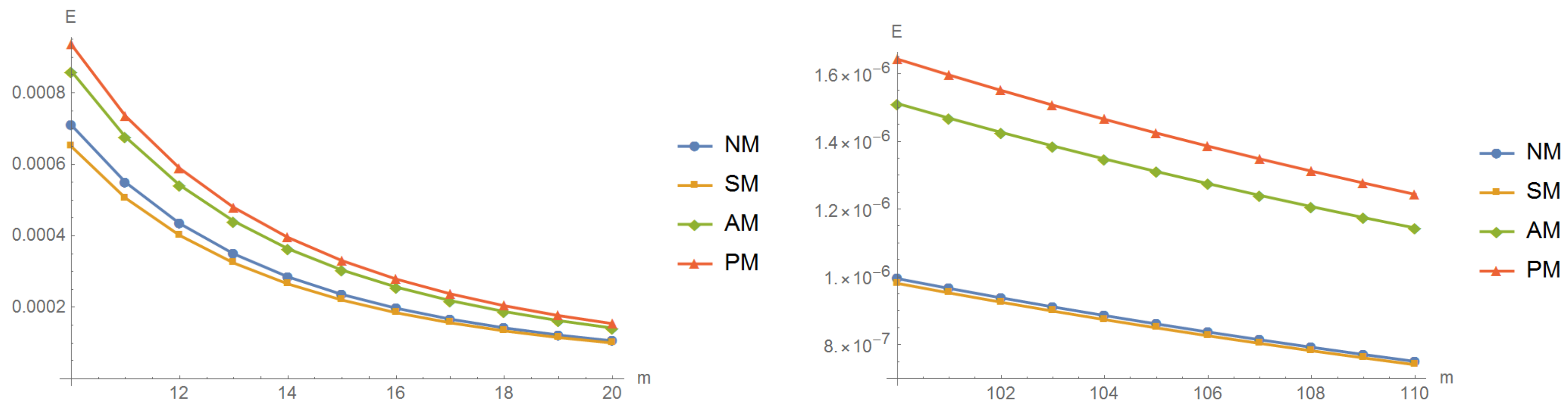
In our comparisons, we applied the Newton’s quadratically convergent iteration expression (NM) and also Steffensen’s method (SM), the third-order expression of Amat et al. (8) denoted by AM, and the presented approach (16) showed by PM, for tackling our nonlinear systems of algebraic equations. This is also plotted in Figure 1 showing the competitiveness of the scheme with memory (16).

5. Computational Tests

The aim of this section is to reveal the application of our proposed nonlinear solver for some practical problems. The software Mathematica 11.0, [24,25] was used for doing all calculations regarding the compared methods. We avoided computing any matrix inverse and the linear systems were solved applying the command $\mathtt{LinearSolver}\left[\right]$. For the implementation of such schemes a possible stopping criterion can be defined based on the residual norm and imposed as follows:

$$\left|\right|A(x^{(k)}){\left|\right|}_2\le \epsilon ,$$

(35)

wherein $\epsilon$ is the required accuracy. $\left|\right|·{\left|\right|}_2$ is the $l^2$ norm.

To confirm the theoretical convergence speed in our numerical tests, we obtain the the numerical rate of convergence by employing the following definition:

$$\rho \approx \frac{\ln (|\left|A(x^{(k+1)})\right|{|}_2/\left|\right|A(x^{(k)})|{|}_2)}{\ln (|\left|A(x^{(k)})\right|{|}_2/\left|\right|A(x^{(k-1)})|{|}_2)}.$$

(36)

5.1. An Academical Test

Example 1.

Here a nonlinear system of equations $A(x)=0$, having complex root is examined as comes next:

$$\begin{array}{c}A(x)=\left\{\begin{array}{c}5\exp (x_1-2)x_2+2{x_7}^{x_{10}}+8{x_3}^{x_4}-5{x_6}^3-x_9,\hfill \\ 5\tan (x_1+2)+\cos ({x_9}^{x_{10}})+{x_2}^3+7{x_3}^4-2{\sin }^3(x_6),\hfill \\ {x_1}^2-x_{10}{x}_5{x}_6{x}_7{x}_8{x}_9+\tan (x_2)+2{x_3}^{x_4}-5{x_6}^3,\hfill \\ 2\tan ({x_1}^2)+2^{x_2}+{x_3}^2-5{x_5}^3-x_6+{x_8}^{\cos (x_9)},\hfill \\ 10{x_1}^2-x_{10}+\cos (x_2)+{x_3}^2-5{x_6}^3-2x_8-4^{x_9},\hfill \\ {\cos }^{-1}({x_1}^2)\sin (x_2)-2x_{10}{x_5}^4{x}_6{x}_9+{x_3}^2,\hfill \\ x_1{x_2}^{x_7}-{x_8}^{x_{10}}+{x_3}^5-5{x_5}^3+x_7,\hfill \\ {\cos }^{-1}(-10x_{10}+x_8+x_9)+x_4\sin (x_2)+x_3-15{x_5}^2+x_7,\hfill \\ 10x_1+{x_3}^2-5{x_5}^2+10{x_6}^{x_8}-\sin (x_7)+2x_9,\hfill \\ x_1\sin (x_2)-2{x_{10}}^{x_8}+x_{10}-5x_6-10x_9,\hfill \end{array}\right.\end{array}$$

(37)

wherein the exact solution just shown up to 10 decimal places as follows:

$$\begin{array}{ccc}\alpha \hfill & \simeq \hfill & (1.3273490437+0.3502924960i,1.058599346-1.748724664i,\hfill \\ & & 1.0276186794-0.0141308051i,3.273950008+0.127828308i,\hfill \\ & & 0.8318243937+0.0017551949i,-0.4853245912+0.6848776400i,\hfill \\ & & 0.1693667630+0.1840917580i,1.534419958-0.321214766i,\hfill \\ & & {2.086379651+0.426342755i,-1.989592331+1.478395393i)}^{*}.\hfill \end{array}$$

(38)

The numerical evidences and the computational order of convergence $\rho$ for this experiment are reported forward in

Table 1. Comparison evidences for Example 1.

Met.	$\parallel \mathit{A}({\mathit{x}}^{(3)})\parallel$	$\parallel \mathit{A}({\mathit{x}}^{(4)})\parallel$	$\parallel \mathit{A}({\mathit{x}}^{(5)})\parallel$	$\parallel \mathit{A}({\mathit{x}}^{(6)})\parallel$	$\parallel \mathit{A}({\mathit{x}}^{(7)})\parallel$	$\parallel \mathit{A}({\mathit{x}}^{(8)})\parallel$	$\parallel \mathit{A}({\mathit{x}}^{(9)})\parallel$	$\mathit{\rho }$
NM	$8.19E-1$	$2.73E-2$	$1.79E-5$	$1.28E-11$	$2.52E-23$	$8.28E-47$	$2.50E-94$	2.02
SM	$7.68E-1$	$1.83E-2$	$7.33E-6$	$5.17E-12$	$1.51E-24$	$2.03E-49$	$3.91E-99$	1.99
AM	$8.50E-2$	$6.50E-6$	$4.98E-17$	$3.68E-50$	$1.26E-149$	$4.83E-448$		3.00
PM	$6.80E-2$	$1.12E-7$	$5.15E-26$	$1.76E-86$	$6.47E-287$			3.31

using 1000 fixed floating point arithmetic and the starting value $x^{(0)}=(1.2+0.3I,1.1-1.9I$, $1.0-0.1I,2.5+0.5I$, $0.8-0.1I,-0.4+1.I$, $0.1+0.1I,1.3-0.7I$, ${2.0+0.5I,-1.9+1.4I)}^{*}$. Here, the residual norm ${\parallel ·\parallel }_2$ is reported.

5.2. An Integral Equation Using a Collocation Approach

Example 2.

The purpose of this test was to examine the performance of the new derivative-free scheme with memory for the following mixed Hammerstein integral equation [6]:

$$y(s)=1+\frac{1}{5}{\int }_0^{1}G(s,t)y{(t)}^{3}dt,$$

(39)

wherein $y\in C[0,1]$, $s,t\in [0,1]$ and the kernel G is defined as follows:

$$G(s,t)=\left\{\begin{array}{c}(1-s)t,t\le s,\hfill \\ s(1-t),t>s.\hfill \end{array}\right.$$

(40)

By employing the well-resulted Gauss-Legendre quadrature formula in discretization of integral equations given in the following form, we will be able to tackle (39):

$${\displaystyle {\int }_0^{1}y(t)dt\approx \sum _{j=1}^{\chi }{w}_{j}y(t_j),}$$

(41)

where the abscissas $t_j$ and the weights $w_j$ were determined via the formula of Gauss–Legendre quadrature.

The lower limit of integration in standard Gauss–Legendre quadrature formula is $-1$. In order to approximate the integral (41) over $[0,1]$, we should map the roots of Legendre polynomials $t_j$ on this segment and scale the weights $w_j$.

Showing the estimation $y(t_i)$ via $x_i$ ($i=1,2,\cdots ,\chi$), one would be able to transfigure the process of solving nonlinear mixed integral equations into a set of nonlinear algebraic equations as comes next:

$${\displaystyle 5x_i-5-\sum _{j=1}^{\chi }{c}_{ij}{x}_j^3=0,i=1,2,\cdots ,\chi ,}$$

(42)

where

$$c_{ij}=\left\{\begin{array}{c}{w}_j{t}_j(1-t_i),ifj\le i,\hfill \\ w_j{t}_i(1-t_j),ifi<j.\hfill \end{array}\right.$$

(43)

For this example, we employed 200 digits floating point in the computations with the stop termination as the following residual norm (35) with $\epsilon ={10}^{-100}$. The initial vector was selected as $x^{(0)}={(3,3,\dots ,3)}^{*}$, while the results are shown in Figure 2 using $\chi =40$ as a list log plot of the function values by performing the cycle. It reveals a stable and fast performance of the new scheme with memory in solving integral equations. Recalling that the Figure 2 can be interpreted only as an error of numerical solution of the system (42) but not the error of solution of the source integral Equation (39).

6. Summary

For derivative-involved iteration schemes in solving nonlinear systems, we use the $m\times m$ Jacobian matrix, i.e., $F^{\prime }(x)$, with entries $F^{\prime }{(x)}_{jk}$$={\partial }_{x_k}{f}_j(x)$. Higher order schemes, such as Chebyshev methods, need higher multi dimensional derivatives which make them less practical. To be more precise, the first Fréchet derivative is a matrix with $m^2$ elements, while the 2nd order Fréchet differentiation has $m^3$ entries (ignoring the symmetric feature).

In this work, we have developed and introduced a variant of Steffensen’s method with memory for tackling nonlinear problems. The scheme consists of two steps and requires the the computation of only one LU factorization which makes its computational efficiency index higher than some of the existing solvers in the literature.

The application of the iteration scheme for nonlinear integral equations via the collocation approach was discussed and its application for other types of nonlinear discretized set of equations obtained from practical problems such as the ones in [26,27] can be investigated similarly.

References

1. Qasim, S.; Ali, Z.; Ahmad, F.; Serra-Capizzano, S.; Ullah, M.Z.; Mahmood, A. Solving systems of nonlinear equations when the nonlinearity is expensive. Comput. Math. Appl. 2016, 71, 1464–1478. [Google Scholar] [CrossRef]
2. Wazwaz, A.-M. Linear and Nonlinear Integral Equations; Higher Education Press: Beijing, China; Springer: Berlin/Heidelberg, Germany, 2011. [Google Scholar]
3. Mashayekhi, S.; Razzaghi, M.; Tripak, O. Solution of the nonlinear mixed Volterra-Fredholm integral equations by hybrid of block-pulse functions and Bernoulli polynomials. Sci. World J. 2014, 2014. [Google Scholar] [CrossRef] [PubMed]
4. Alzahrani, E.O.; Al-Aidarous, E.S.; Younas, A.M.M.; Ahmad, F.; Ahmad, S.; Ahmad, S. A higher order frozen Jacobian iterative method for solving Hamilton-Jacobi equations. J. Nonlinear Sci. Appl. 2016, 9, 6210–6227. [Google Scholar] [CrossRef] [Green Version]
5. Soleymani, F. Pricing multi–asset option problems: A Chebyshev pseudo–spectral method. BIT Numer. Math. 2019, 59, 243–270. [Google Scholar] [CrossRef]
6. Ortega, J.M.; Rheinboldt, W.C. Iterative Solution of Nonlinear Equations in Several Variables; Academic Press: New York, NY, USA, 1970. [Google Scholar]
7. Noda, T. The Steffensen iteration method for systems of nonlinear equations. Proc. Jpn. Acad. 1987, 63, 186–189. [Google Scholar] [CrossRef]
8. Grau-Sánchez, M.; Grau, À.; Noguera, M. On the computational efficiency index and some iterative methods for solving systems of nonlinear equations. J. Comput. Appl. Math. 2011, 236, 1259–1266. [Google Scholar] [CrossRef] [Green Version]
9. Traub, J.F. Iterative Methods for the Solution of Equations; Prentice Hall: New York, NY, USA, 1964. [Google Scholar]
10. Amat, S.; Busquier, S. Convergence and numerical analysis of a family of two-step Steffensen’s methods. Comput. Math. Appl. 2005, 49, 13–22. [Google Scholar] [CrossRef]
11. Soleymani, F.; Sharifi, M.; Shateyi, S.; Haghani, F.K. A class of Steffensen-type iterative methods for nonlinear systems. J. Appl. Math. 2014, 2014. [Google Scholar] [CrossRef]
12. Babajee, D.K.R.; Dauhoo, M.Z.; Darvishi, M.T.; Barati, A. A note on the local convergence of iterative methods based on Adomian decomposition method and 3-node quadrature rule. Appl. Math. Comput. 2008, 200, 452–458. [Google Scholar] [CrossRef]
13. Alaidarous, E.S.; Ullah, M.Z.; Ahmad, F.; Al-Fhaid, A.S. An efficient higher-order quasilinearization method for solving nonlinear BVPs. J. Appl. Math. 2013, 2013. [Google Scholar] [CrossRef]
14. Hanaç, E. The phase plane analysis of nonlinear equation. J. Math. Anal. 2018, 9, 89–97. [Google Scholar]
15. Hasan, P.M.A.; Sulaiman, N.A. Numerical treatment of mixed Volterra-Fredholm integral equations using trigonometric functions and Laguerre polynomials. ZANCO J. Pure Appl. Sci. 2018, 30, 97–106. [Google Scholar]
16. Qasim, U.; Ali, Z.; Ahmad, F.; Serra-Capizzano, S.; Ullah, M.Z.; Asma, M. Constructing frozen Jacobian iterative methods for solving systems of nonlinear equations, associated with ODEs and PDEs using the homotopy method. Algorithms 2016, 9, 18. [Google Scholar] [CrossRef]
17. Ahmad, F.; Soleymani, F.; Khaksar Haghani, F.; Serra-Capizzano, S. Higher order derivative-free iterative methods with and without memory for systems of nonlinear equations. Appl. Math. Comput. 2017, 314, 199–211. [Google Scholar] [CrossRef]
18. Bellavia, S.; Bertaccini, D.; Morini, B. Nonsymmetric preconditioner updates in Newton-Krylov methods for nonlinear systems. SIAM J. Sci. Comput. 2011, 33, 2595–2619. [Google Scholar] [CrossRef]
19. Bellavia, S.; Morini, B.; Porcelli, M. New updates of incomplete LU factorizations and applications to large nonlinear systems. Optim. Methods Softw. 2014, 29, 321–340. [Google Scholar] [CrossRef]
20. Bertaccini, D.; Durastante, F. Interpolating preconditioners for the solution of sequence of linear systems. Comput. Math. Appl. 2016, 72, 1118–1130. [Google Scholar] [CrossRef]
21. Sharma, J.R.; Kumar, D.; Argyros, I.K.; Magreñán, Á.A. On a bi-parametric family of fourth order composite Newton-Jarratt methods for nonlinear systems. Mathematics 2019, 7, 492. [Google Scholar] [CrossRef]
22. Cordero, A.; Hueso, J.L.; Martínez, E.; Torregrosa, J.R. A modified Newton-Jarratt’s composition. Numer. Algorithms 2010, 55, 87–99. [Google Scholar] [CrossRef]
23. Montazeri, H.; Soleymani, F.; Shateyi, S.; Motsa, S.S. On a new method for computing the numerical solution of systems of nonlinear equations. J. Appl. Math. 2012, 2012, 1–15. [Google Scholar] [CrossRef]
24. Sánchez León, J.G. Mathematica Beyond Mathematics: The Wolfram Language in the Real World; Taylor & Francis Group: Boca Raton, FL, USA, 2017. [Google Scholar]
25. Wagon, S. Mathematica in Action, 3rd ed.; Springer: Berlin, Germany, 2010. [Google Scholar]
26. Soheili, A.R.; Soleymani, F. Iterative methods for nonlinear systems associated with finite difference approach in stochastic differential equations. Numer. Algorithms 2016, 71, 89–102. [Google Scholar] [CrossRef]
27. Soleymani, F.; Barfeie, M. Pricing options under stochastic volatility jump model: A stable adaptive scheme. Appl. Numer. Math. 2019, 145, 69–89. [Google Scholar] [CrossRef]
Figure 1. The comparison of flops-like efficiency indices for various schemes with and without memory by changing m.
Mathematics 07 00637 g001
Figure 2. Error history for solving the integral equation in Example 2 using PM (Performed by Mathematica).
Mathematics 07 00637 g002