An Optimal Eighth-Order Family of Iterative Methods for Multiple Roots

Abstract

In this paper, we introduce a new family of efficient and optimal iterative methods for finding multiple roots of nonlinear equations with known multiplicity $(m\ge 1)$. We use the weight function approach involving one and two parameters to develop the new family. A comprehensive convergence analysis is studied to demonstrate the optimal eighth-order convergence of the suggested scheme. Finally, numerical and dynamical tests are presented, which validates the theoretical results formulated in this paper and illustrates that the suggested family is efficient among the domain of multiple root finding methods.

1. Introduction

The problem of solving nonlinear equation is recognized to be very old in history as many practical problems which arise are nonlinear in nature. Various one-point and multi-point methods are presented to solve nonlinear equations or systems of nonlinear equations [1,2,3]. The above-cited methods are designed for the simple root of nonlinear equations but the behavior of these methods is not similar when dealing with multiple roots of nonlinear equations. The well known Newton’s method with quadratic convergence for simple roots of nonlinear equations decays to first order when dealing with multiple roots of nonlinear equations. These problems lead to minor troubles such as greater computational cost and severe troubles such as no convergence at all. The prior knowledge of multiplicity of roots make it simpler to manage these troubles. The strange behavior of the iterative methods while dealing with multiple roots has been well known since 19th century in the least when Schröder [4] developed a modification of classical Newton’s method to conserve its second order of convergence for multiple roots. The nonlinear equations with multiple roots commonly arise from different topics such as complex variables, fractional diffusion or image processing, applications to economics and statistics (Lēvy distributions), etc. By knowing the practical nature of multiple root finders, various one-point and multi-point root solvers have been developed in recent past [5,6,7,8,9,10,11,12,13,14,15,16,17,18] but most of them are not optimal as defined by Kung and Traub [19], who stated that an optimal without memory method can achieve its convergence order at the most $2^n$ requiring $n+1$ evaluations of functions or derivatives. As stated by Ostrowski [1], if an iterative method possess order of convergence as O and total number of functional evaluations is n per iterative step, then the index defined by $E=O^{1/n}$ is recognized as efficiency index of an iterative method.

Sharma and Sharma [17] proposed the following optimal fourth-order multiple root finder with known multiplicity m as follows:

$$\begin{array}{cc}\hfill y_n& =x_n-\frac{2m}{m+2}·\frac{f\left(x_n\right)}{f^{\prime }\left(x_n\right)},m>1\\ \hfill x_{n+1}& =x_n-\frac{m}{8}\mathsf{\Phi }\left(x_n\right)\frac{f\left(x_n\right)}{f^{\prime }\left(x_n\right)},\end{array}$$

where $\mathsf{\Phi }\left(x_n\right)=\left\{(m^3-4m+8)-{(m+2)}^2{\left(\frac{m}{m+2}\right)}^m\frac{f^{\prime }\left(x_n\right)}{f^{\prime }\left(y_n\right)}\times 2(m-1)(m+2){\left(\frac{m}{m+2}\right)}^m\frac{f^{\prime }\left(x_n\right)}{f^{\prime }\left(y_n\right)}\right\}.$

A two-step sixth-order non-optimal family for multiple roots presented by Geum et al. [9] is given by:

$$\begin{array}{ccc}\hfill y_n& =& x_n-m·\frac{f\left(x_n\right)}{f^{\prime }\left(x_n\right)},m>1,\hfill \\ \hfill x_{n+1}& =& y_n-Q(r_n,s_n)·\frac{f\left(y_n\right)}{f^{\prime }\left(y_n\right)},\hfill \end{array}$$

(1)

where, $r_n=\sqrt[m]{\frac{f\left(y_n\right)}{f\left(x_n\right)}},s_n=\sqrt[m-1]{\frac{f^{\prime }\left(y_n\right)}{f^{\prime }\left(x_n\right)}}$ and $Q:{\mathbb{C}}^2\to \mathbb{C}$ is holomorphic in a neighborhood of $(0,0)$. The following is a special case of their family:

$$\begin{array}{ccc}\hfill y_n& =& x_n-m·\frac{f\left(x_n\right)}{f^{\prime }\left(x_n\right)},n\ge 0,m>1,\hfill \\ \hfill x_{n+1}& =& y_n-m\left[1+2(m-1)(r_n-s_n)-4r_n{s}_n+s_n^2\right]·\frac{f\left(y_n\right)}{f^{\prime }\left(y_n\right)}.\hfill \end{array}$$

(2)

Another non-optimal family of three-point sixth-order methods for multiple roots by Geum et al. [10] is given as follows:

$$\begin{array}{ccc}\hfill y_n& =& x_n-m·\frac{f\left(x_n\right)}{f^{\prime }\left(x_n\right)},m\ge 1,\hfill \\ \hfill w_n& =& y_n-m·G\left(p_n\right)·\frac{f\left(x_n\right)}{f^{\prime }\left(x_n\right)},\hfill \\ \hfill x_{n+1}& =& w_n-m·K(p_n,v_n,)·\frac{f\left(x_n\right)}{f^{\prime }\left(x_n\right)},\hfill \end{array}$$

(3)

where $p_n=\sqrt[m]{\frac{f\left(y_n\right)}{f\left(x_n\right)}}$ and $v_n=\sqrt[m]{\frac{f\left(w_n\right)}{f\left(x_n\right)}}.$ The weight functions $G:\mathbb{C}\to \mathbb{C}$ is analytic in a neighborhood of 0 and $K:{\mathbb{C}}^2\to \mathbb{C}$ is holomorphic in a neighborhood of $(0,0)$. The following is a special case of the family in Equation (3):

$$\begin{array}{ccc}\hfill y_n& =& x_n-m·\frac{f\left(x_n\right)}{f^{\prime }\left(x_n\right)},m\ge 1,\hfill \\ \hfill w_n& =& y_n-m·\left[1+p_n+2p_n^2\right]·\frac{f\left(x_n\right)}{f^{\prime }\left(x_n\right)},\hfill \\ \hfill x_{n+1}& =& w_n-m·\left[1+p_n+2p_n^2+(1+2p_n)v_n\right]·\frac{f\left(x_n\right)}{f^{\prime }\left(x_n\right)}.\hfill \end{array}$$

(4)

The families in Equations (1) and (3) require four evaluations of function to produce convergence of order six having efficiency index $6^{\frac{1}{4}}=1.5650$ and therefore are not optimal in the sense of the Kung–Traub conjecture [19].

Recently, Behl et al. [20] presented a multiple root finding family of iterative methods possessing convergence order eight given as:

$$\begin{array}{ccc}\hfill y_n& =& x_n-m\frac{f\left(x_n\right)}{f^{\prime }\left(x_n\right)},m\ge 1,\hfill \\ \hfill z_n& =& y_n-u_{n}Q\left(h_n\right)\frac{f\left(x_n\right)}{f^{\prime }\left(x_n\right)},\hfill \\ \hfill x_{n+1}& =& z_n-u_n{t}_{n}G(h_n,t_n)\frac{f\left(x_n\right)}{f^{\prime }\left(x_n\right)},\hfill \end{array}$$

(5)

where the functions $Q:\mathbb{C}\to \mathbb{C}$ and $G:{\mathbb{C}}^2\to \mathbb{C}$ are restricted to be analytic functions in the regions nearby $\left(0\right)$ and $(0,0),$ respectively, with $u_n={\left(\frac{f\left(y_n\right)}{f\left(x_n\right)}\right)}^{\frac{1}{m}},$$h_n=\frac{u_n}{a_1+a_2{u}_n}$ and $t_n={\left(\frac{f\left(z_n\right)}{f\left(y_n\right)}\right)}^{\frac{1}{m}},$ being $a_1$ and $a_2$ complex non-zero free parameters.

We take Case (27) for ($a_1$$=1$, $a_2=1$, $G_{02}=0)$ from the family of Behl et al. [20] and represent it by $BM$ given by:

$$\begin{array}{ccc}\hfill y_n& =& x_n-m\frac{f\left(x_n\right)}{f^{\prime }\left(x_n\right)},\hfill \\ \hfill z_n& =& y_n-\left(m+2h_{n}m+\frac{1}{2}{h}_n^2(4m+2m)\right)\frac{f\left(x_n\right)}{f^{\prime }\left(x_n\right)}{u}_n\hfill \\ \hfill x_{n+1}& =& z_n-\left(m+m{t}_n+3m{h}_n^2+m{h}_n(2+4t_n+h_n)\right)\frac{f\left(x_n\right)}{f^{\prime }\left(x_n\right)}{u}_n{t}_n.\hfill \end{array}$$

(6)

Most recently, another optimal eighth-order scheme presented by Zafar et al. [21] is given as:

$$\begin{array}{ccc}\hfill y_n& =& x_n-m\frac{f\left(x_n\right)}{f^{\prime }\left(x_n\right)},m\ge 1,\hfill \\ \hfill z_n& =& y_n-m{u}_{n}H\left(u_n\right)\frac{f\left(x_n\right)}{f^{\prime }\left(x_n\right)},\hfill \\ \hfill x_{n+1}& =& z_n-u_n{t}_n(B_1+B_2{u}_n)P\left(t_n\right)G\left(w_n\right)\frac{f\left(x_n\right)}{f^{\prime }\left(x_n\right)},\hfill \end{array}$$

(7)

where $B_1$,$B_2\in \mathbb{R}$ are suppose to be free parameters and weight functions $H:\mathbb{C}\to \mathbb{C},$$P:\mathbb{C}\to \mathbb{C}$ and $G:\mathbb{C}\to \mathbb{C}$ are restricted to be analytic in the regions nearby 0 with $u_n={\left(\frac{f\left(y_n\right)}{f\left(x_n\right)}\right)}^{\frac{1}{m}},$$t_n={\left(\frac{f\left(z_n\right)}{f\left(y_n\right)}\right)}^{\frac{1}{m}}$ and $w_n={\left(\frac{f\left(z_n\right)}{f\left(x_n\right)}\right)}^{\frac{1}{m}}.$

From the eighth-order family of Zafar et al. [21], we consider the following special case denoted by $ZM$:

$$\begin{array}{ccc}\hfill y_n& =& x_n-m\frac{f\left(x_n\right)}{f^{\prime }\left(x_n\right)},\hfill \\ \hfill z_n& =& y_n-m{u}_n\left(6u_n^3-u_n^2+2u_n+1\right)\frac{f\left(x_n\right)}{f^{\prime }\left(x_n\right)},\hfill \\ \hfill x_{n+1}& =& z_n-m{u}_n{t}_n\left(1+2u_n\right)(1+t_n)(1+2w_n)\frac{f\left(x_n\right)}{f^{\prime }\left(x_n\right)}.\hfill \end{array}$$

(8)

The class of iterative methods referred as optimal is significant as compared to non-optimal methods due to their speed of convergence and efficiency index. Therefore, there was a need to develop optimal eighth-order schemes for finding multiple zeros ($m>1$) and simple zeros ($m=1$) due to their competitive efficiencies and order of convergence [1]; in addition, fewer iterations are needed to get desired accuracy as compared to iterative methods having order four and six given by Sharma and Geum [9,10,17], respectively. In this paper, our main concern is to find the optimal iterative methods for multiple root $\mu$ with known multiplicity $m\in \mathbb{N}$ of an adequately differentiable nonlinear function $f:I\subseteq \mathbb{R}\to \mathbb{R}$, where I represents an open interval. We develop an optimal eighth-order zero finder for multiple roots with known multiplicity $m\ge 1$. The beauty of the method lies in the fact that developed scheme is simple to implement with minimum possible number of functional evaluations. Four evaluations of the function are needed to obtain a family of convergence order eighth having efficiency index $8^{\frac{1}{4}}=1.6817$.

The rest of the paper is organized as follows. In Section 2, we present the newly developed optimal iterative family of order eight for multiple roots of nonlinear equations. The discussion of analysis of convergence is also given in this section. In Section 3, some special cases of newly developed eighth-order schemes are presented. In Section 4, numerical results and comparison of the presented schemes with existing schemes of its domain is discussed. Concluding remarks are given in Section 5.

2. Development of the Scheme and Convergence Analysis

In this section, we suggest a new family of eighth-order method with known multiplicity $m\ge 1$ of the required multiple root as follows:

$$\begin{array}{ccc}\hfill y_n& =& x_n-m·\frac{f\left(x_n\right)}{f^{\prime }\left(x_n\right)},n\ge 0,\hfill \\ \hfill z_n& =& y_n-m·t·H\left(t\right)·\frac{f\left(x_n\right)}{f^{\prime }\left(x_n\right)},\hfill \\ \hfill x_{n+1}& =& z_n-m·t·L(s,u)·\frac{f\left(x_n\right)}{f^{\prime }\left(x_n\right)},\hfill \\ \hfill \mathrm{where}t& =& \sqrt[m]{\frac{f\left(y_n\right)}{f\left(x_n\right)}},s=\sqrt[m]{\frac{f\left(z_n\right)}{f\left(y_n\right)}},u=\sqrt[m]{\frac{f\left(z_n\right)}{f\left(x_n\right)}}.\hfill \end{array}$$

(9)

where the function $H:\mathbb{C}\to \mathbb{C}$ is restricted to be analytic function in the regions nearby 0 and weight function $L:{\mathbb{C}}^2\to \mathbb{C}$ is holomorphic in the regions nearby $(0,0)$ and $t,s$ and $u$ are $one$-$to$-m multiple-valued functions.

In the next theorem, it is demonstrated that the proposed scheme in Equation (9) achieves the optimal eighth order of convergence without increasing the number of functional evaluations.

Theorem 1.

Suppose $x=\mu$ (say) is a multiple root having multiplicity $m\ge 1$ of an analytic function $f:\mathbb{C}\to \mathbb{C}$ in the region enclosing a multiple zero μ of $f\left(x\right).$ Which implies that the family of iterative methods defined by Equation (9) has convergence of order eighth when the following conditions are fulfilled:

$$H_0=1,H_1=2,H_2=-2,H_3=36,L_{00}=0,L_{10}=1,L_{01}=2,L_{11}=4,L_{20}=2.$$

(10)

Then, the proposed scheme in Equation (9) satisfies the following error equation:

$$\begin{array}{ccc}\hfill e_{n+1}& =& \frac{1}{24m^7}\left\{c_1(c_1^2(11+m)-2m{c}_2)\right((677+108m+7m^2)c_1^4\hfill \\ & & -24m(9+m)c_1^2{c}_2+12m^2{c}_2^2+12m^2{c}_1{c}_3\left)e_n^8\right\}+O\left(e_n^9\right),\hfill \end{array}$$

(11)

where $e_n=x_n-\mu$ and $c_k=\frac{m!}{(m+k)!}\frac{f^{(m+k)}\left(\mu \right)}{f^{\left(m\right)}\left(\mu \right)},k=1,2,3,···.$

Proof. 

Suppose $x=\mu$ is a multiple root of $f\left(x\right)$. We expand $f\left(x_n\right)$ and $f^{\prime }\left(x_n\right)$ by Taylor’s series expansion about $x=\mu$ using Mathematica (Computer based algebra software), to get

$$f\left(x_n\right)=\frac{f^{\left(m\right)}\left(\mu \right)}{m!}{e}_n^m\left(1+c_1{e}_n+c_2{e}_n^2+c_3{e}_n^3+c_4{e}_n^4+c_5{e}_n^5+c_6{e}_n^6+c_7{e}_n^7+c_8{e}_n^8+O\left(e_n^9\right)\right),$$

(12)

and

$$\begin{array}{cc}\hfill f^{\prime }\left(x_n\right)& =\frac{f^{\left(m\right)}\left(\mu \right)}{m!}{e}_n^{m-1}m+c_1(m+1)e_n+c_2(m+2)e_n^2+c_3(m+3)e_n^3+c_4(m+4)e_n^4\\ & +c_5(m+5)e_n^5+c_6(m+6)e_n^6+c_7(m+7)e_n^7+c_8(m+8)e_n^8+O\left(e_n^9\right),\end{array}$$

respectively. By utilizing the above Equations (11) and (12) in the first substep of Equation (9), we obtain

$$y_n-\mu =\frac{c_1{e}_n^2}{m}+\frac{(2c_{2}m-c_1^2(m+1))e_n^3}{m^2}+\sum \underset{k=0}{\overset{4}{lim}}{G}_k{e}_n^{k+4}+O\left(e_n^9\right),$$

(13)

where $G_k=G_k(m,c_1,c_2,\dots ,c_8)$ are expressed in terms of $m,c_1,c_2,c_3,\dots ,c_8$ and the two coefficients $G_0$ and $G_1$ can be explicitly written as $G_0=\frac{1}{m^3}\{3c_3{m}^2+c_1^3{(m+1)}^2-c_1{c}_{2}m(3m+4)\}$ and $G_1=-\frac{1}{m^4}\{c_1^4{(m+1)}^3-2c_2{c}_1^{2}m(2m^2+5m+3)+2c_3{c}_1{m}^2(2m+3)+2m^2(c_2^2(m+2)-2c_{4}m)\}.$ By Taylor’s expansion, we get

$$f\left(y_n\right)=f^{\left(m\right)}\left(\mu \right)e_n^{2m}\left[\frac{{\left(\frac{c_1}{m}\right)}^m}{m!}+\frac{(2m{c}_2-(m+1)c_1^2){\left(\frac{c_1}{m}\right)}^m{e}_n}{c_{1}m!}+\sum _{k=0}^6{\overline{G}}_k{e}_n^{k+2}+O\left(e_n^9\right)\right].$$

(14)

By using Equations (12) and (14), we get

$$u=\frac{c_1{e}_n}{m}+\frac{(2m{c}_2-(m+2)c_1^2)e_n^2}{m^2}+{\psi }_1{e}_n^3+{\psi }_2{e}_n^4+{\psi }_3{e}_n^5+O\left(e_n^6\right),$$

(15)

where ${\psi }_1=\frac{1}{2m^3}[c_1^3(2m^2+7m+7)+6c_3{m}^2-2c_1{c}_{2}m(3m+7)],$ ${\psi }_2=-\frac{1}{6m^4}[c_1^4(6m^3+29m^2+51m+34)-6c_2{c}_1^{2}m(4m^2+16m+17)+12c_1{c}_3{m}^2(2m+5)+12m^2(c_2^2(m+3)-2c_{4}m)],$ ${\psi }_3=\frac{1}{24m^5}[-24m^3(c_2{c}_3(5m+17)-5c_{5}m)+12c_3{c}_1^2{m}^2(10m^2+43m+49)+12c_1{m}^2\{c_2^2(10m^2+47m+53)-2c_{4}m(5m+13)\}-4c_2{c}_1^{3}m(30m^3+163m^2+306m+209)+c_1^5(24m^4+146m^3+355m^2+418m+209)].$

Taylor series of $H\left(t\right)$ about 0 is given by:

$$H\left(t\right)=H_0+H_{1}t+\frac{H_2}{2!}{t}^2+\frac{H_3}{3!}{t}^3+O\left(e_n^4\right)$$

(16)

where $H_j=H^j\left(0\right)$ for $0\le j\le 3.$ Inserting Equations (13)–(16) in the second substep of the scheme in Equation (9), we get

$$\begin{array}{ccc}\hfill z_n& =& \mu +\frac{-(1+H_0)c_1{e}_n^2}{m}-\frac{(1+H_1+m-H_0(3+m)c_1^2)+2(-1+H_0)m{c}_2)e_n^3}{m^2}\hfill \\ & & +\frac{1}{2m^3}\left[(2+10H_1-H_2+4m+4H_{1}m+2m^2-H_0(13+11m+2m^2))c_1^3\right.\hfill \\ & & \left.+2m(-4-4H_1-3m+H_0(11+3m)c_1{c}_2-6(-1+H_0)m^2{c}_3)e_n^4\right]+z_5{e}_n^5\hfill \\ & & +z_6{e}_n^6+z_7{e}_n^7+O\left(e_n^8\right).\hfill \end{array}$$

By selecting $H_0=1$ and $H_1=2$, we obtain

$$z_n=\mu +\frac{(c_1^3(9-H_2+m)-2m{c}_1{c}_2)}{2m^3}{e}_n^4+z_5{e}_n^5+z_6{e}_n^6+z_7{e}_n^7+O\left(e_n^8\right),$$

(17)

where $z_5=-\frac{1}{6m^4}\{c_1^4(125+H_3+84m+7m^2-3H_2(7+3m)+6m(-3H_2+4(7+m))c_1^2{c}_2+12c_2^2{m}^2+12c_2{c}_{1}m)$, $z_6=\frac{1}{24m^5}\{1507+1850m+677m^2+46m^3+4H_3(9+4m)-6H2(59+53m+12m^2))c_1^5-4m(925+8H_3+594m+53m^2-3H_2(53+21m)c_1^3{c}_2$ $+12m^2(83-9H_2+13m)c_1^2{c}_3-168m^3{c}_2{c}_3+12m^2{c}_1(115-12H2+17m)c_2^2-6m{c}_4)$ and $z_7=-\{12c_1^2{c}_3{m}^2(36\beta +13m+11)+(37-168c_2{c}_3{m}^3+4c_1^3{c}_{2}m(96{\beta }^2+252\beta +53m^2+18(14\beta +5)m)+12c_1{m}^2(c_2^2(48\beta +17m+19)-6c_{4}m)\}.$

Again, we use the Taylor’s expansion for Equation (17) to get:

$$\begin{array}{cc}\hfill f\left(z_n\right)& =f^{\left(m\right)}\left(\mu \right)e_n^{4m}\frac{2^{-m}{\left(\frac{c_1^3(9-H_2+m)-2m{c}_1{c}_2}{m^3}\right)}^m}{m!}-\frac{\left(2^{-m}{\left(\frac{c_1^3(9-H_2+m)-2m{c}_1{c}_2}{m^3}\right)}^{m-1}{\rho }_0\right)}{3(m^{3}m!)}{e}_n\\ & +\sum \underset{j=0}{\overset{7}{lim}}{\overline{H}}_j{e}_n^{j+1}+O\left(e_n^9\right),\end{array}$$

where ${\rho }_0=c_1^4(125+H_3+84m+7m^2-3H_2(7+3m))c_1^4-6m(-3H2+4(7+m))c_1^2{c}_2+12m^2{c}_2^2+12c_3{c}_1{m}^2).$ With the help of Equations (12) and (18), we have

$$s=\frac{c_1^2(9-H_2+m)-2m{c}_2}{2m^2}{e}_n^2+{\rho }_1{e}_n^3+{\rho }_2{e}_n^4+{\rho }_3{e}_n^5+O\left(e_n^6\right),$$

(18)

where

$${\rho }_1=-\frac{1}{6m^3}\{c_1^3(98+H_3+4m^2+54m-6H_2(3+m)-12m(9-H_2+m)c_1{c}_2+12m^2{c}_3\},$$

$${\rho }_2=\frac{1}{24m^4}899+1002m+313m^2+18m^3+4H_3(8+3m)-6H_2(43+33m+6m^2))c_1^4-$$

$$12m(167+2H_3+87m+6m^2-H_2(33+10m)c_1^2{c}_2+24m^2(26-3H_2+3m)c_1{c}_3+$$

$$12m^2(c_2^2(35-4H_2+3m)-6m{c}_4)$$

and ${\rho }_3=-\frac{1}{60m^5}[-4257-7270m-4455m^2-101m^3-48m^4-10H_3(37+30m+6m^2)+30H_2(60+75m+31m^2+4m^3)c_1^5$ $+10m(1454+60H_3+1548m+21H_{3}m+454m^2+24m^3-18H_2(25+18m+3m^2)c_1^3{c}_2-30m^2(234+3H_3+118m+8m^2-2H2(24+7m)c_1^2{c}_3-60m^2{c}_1(141+2H_3+67m+4m^2-2H_2(15+4m)c_2^2+2(-17+2H_2-2m)m{c}_4)-120m^3(-25+3H_2-2m)c_2{c}_3+2m{c}_5\}+\left(\frac{1}{720m^6}\right)$ $((102047+180H_2^2+204435m+187055m^2+81525m^3+14738m^4+600m^5+40H_3(389+498m+214m^2+30m^3)-45H_2(1223+2030m+1353m^2+394m^3+40m^4))$ $-30m(13629+22190m+12915m^2+2746m^3+120m^4+16H_3(83+64m+12m^2)-6H_2(1015+1209m+470m^2+56m^3))+120m^2(2063+2088m+589m^2+30m^3+H_3(88+30m)-18H_2+(36+25m+4m^2))$ $+80m^2(2323+2348m+635m^2+30m^3+4H_3(28+9m)-3H_2(259+173m+26m^2))-2m(303+4H_3+149m+10m^2-9H_2(7+2m))-720m^3\left((393+6H_3+178m+10m^2-H_2(87+22m))\right]+(-42+5H_2-5m)m{c}_5)$ $+20m^3((-473-8H_3-195m-10m^2+12H_2(9+2m))c_2{c}_3+6m(65-8H2+5m)c_2+3m(71-9H2+5m)c_{10}m{c}_6.$

Since it is obvious from Equation (15) that u possess order $e_n$, the expansion of weight function $L_f(s,u)$ by Taylor’s series is possible in the regions nearby origin given as follows:

$$L(s,u)=L_{00}+s{L}_{10}+u{L}_{01}+su{L}_{11}+\frac{s^2}{2!}{L}_{20}$$

(19)

where ${\left.L_{i,j}=\frac{1}{i!j!}\frac{{\partial }^{i+j}}{\partial s^j\partial u^j}L(s,u)\right|}_{(0,0)}.$ By using Equations (12)–(19) in the proposed scheme in Equation (9), we have

$$e_{n+1}=M_2{e}_n^2+M_3{e}_n^3+M_4{e}_n^4+M_5{e}_n^5+M_6{e}_n^6+M_7{e}_n^7+O\left(e_n^8\right),$$

(20)

where the coefficients $M_i(2\le i\le 7)$ depend generally on m and the parameters $L_{i,j}$. To obtain at least fifth-order convergence, we have to choose $L_{00}=0,L_{10}=1$ and get

$$e_{n+1}=\frac{((-2+L_{01})c_1^2((-9+H_2-m)c_1^2+2m{c}_2)}{2m^4}{e}_n^5+{\overline{M}}_6{e}_n^6+{\overline{M}}_7{e}_n^7+O\left(e_n^8\right).$$

where the coefficients ${\overline{M}}_i(6\le i\le 7)$ depend generally on m and the parameters $L_{i,j}.$ To obtain eighth-order convergence, we are restricted to choosing the values of parameters given by:

$$H_2=-2,H_3=36,L_{00}=0,L_{10}=1,L_{01}=2,L_{20}=2,L_{11}=4.$$

(21)

This leads us to the following error equation:

$$\begin{array}{ccc}\hfill e_{n+1}& =& \frac{1}{24m^7}\left[c_1(c_1^2(11+m)-2m{c}_2)\right((677+108m+7m^2)c_1^4-24m(9+m)c_1^2{c}_2\hfill \\ & & +12m^2{c}_2^2+12m^2{c}_1{c}_3\left)\right]e_n^8+O\left(e_n^9\right).\hfill \end{array}$$

(22)

The above error equation (Equation (22)) confirms that the presented scheme in Equation (9) achieves optimal order of convergence eight by utilizing only four functional evaluations (using $f\left(x_n\right),f^{\prime }\left(x_n\right),f\left(y_n\right)$ and $f\left(z_n\right)$) per iteration. □

3. Special Cases of Weight Functions

From Theorem 1, several choices of weight functions can be obtained. We have considered the following:

Case 1: The polynomial form of the weight function satisfying the conditions in Equation (10) can be represented as:

$$\begin{array}{ccc}\hfill H\left(t\right)& =& 1+2t-t^2+6t^3\hfill \\ \hfill L(s,u)& =& s+2u+4su+s^2\hfill \end{array}$$

(23)

The particular iterative method related to Equation (23) is given by:

SM-1:

$$\begin{array}{ccc}\hfill y_n& =& x_n-m·\frac{f\left(x_n\right)}{f^{\prime }\left(x_n\right)},n\ge 0,\hfill \\ \hfill z_n& =& y_n-m·t·(1+2t-t^2+6t^3)\frac{f\left(x_n\right)}{f^{\prime }\left(x_n\right)},\hfill \\ \hfill x_{n+1}& =& z_n-m·t·(s+s^2+2u+4su)·\frac{f\left(x_n\right)}{f^{\prime }\left(x_n\right)}\hfill \\ \hfill \mathrm{where}t& =& \sqrt[m]{\frac{f\left(y_n\right)}{f\left(x_n\right)}},s=\sqrt[m]{\frac{f\left(z_n\right)}{f\left(y_n\right)}},u=\sqrt[m]{\frac{f\left(z_n\right)}{f\left(x_n\right)}}\hfill \end{array}$$

(24)

Case 2: The second suggested form of the weight functions in which $H\left(t\right)$ is constructed using rational weight function satisfying the conditions in Equation (10) is given by:

$$\begin{array}{ccc}\hfill H\left(t\right)& =& \frac{1+8t+11t^2}{1+6t}\hfill \\ \hfill L(s,u)& =& s+2u+4su+s^2\hfill \end{array}$$

(25)

The corresponding iterative method in Equation (25) can be presented as:

SM-2:

$$\begin{array}{ccc}\hfill y_n& =& x_n-m·\frac{f\left(x_n\right)}{f^{\prime }\left(x_n\right)},n\ge 0,\hfill \\ \hfill z_n& =& y_n-m·t·\left(\frac{1+8t+11t^2}{1+6t}\right)\frac{f\left(x_n\right)}{f^{\prime }\left(x_n\right)},\hfill \\ \hfill x_{n+1}& =& z_n-m·t·(s+s^2+2u+4su)·\frac{f\left(x_n\right)}{f^{\prime }\left(x_n\right)}\hfill \\ \hfill \mathrm{where}t& =& \sqrt[m]{\frac{f\left(y_n\right)}{f\left(x_n\right)}},s=\sqrt[m]{\frac{f\left(z_n\right)}{f\left(y_n\right)}},u=\sqrt[m]{\frac{f\left(z_n\right)}{f\left(x_n\right)}}\hfill \end{array}$$

(26)

Case 3: The third suggested form of the weight function in which $H\left(t\right)$ is constructed using trigonometric weight satisfying the conditions in Equation (10) is given by:

$$\begin{array}{ccc}\hfill H\left(t\right)& =& \frac{5+18t}{5+8t-11t^2}\hfill \\ \hfill L(s,u)& =& s+2u+4su+s^2\hfill \end{array}$$

(27)

The corresponding iterative method obtained using Equation (27) is given by:

SM-3:

$$\begin{array}{ccc}\hfill y_n& =& x_n-m·\frac{f\left(x_n\right)}{f^{\prime }\left(x_n\right)},n\ge 0,\hfill \\ \hfill z_n& =& y_n-m·t·\left(\frac{5+18t}{5+8t-11t^2}\right)\frac{f\left(x_n\right)}{f^{\prime }\left(x_n\right)},\hfill \\ \hfill x_{n+1}& =& z_n-m·t·(s+s^2+2u+4su)·\frac{f\left(x_n\right)}{f^{\prime }\left(x_n\right)}\hfill \\ \hfill \mathrm{where}t& =& \sqrt[m]{\frac{f\left(y_n\right)}{f\left(x_n\right)}},s=\sqrt[m]{\frac{f\left(z_n\right)}{f\left(y_n\right)}},u=\sqrt[m]{\frac{f\left(z_n\right)}{f\left(x_n\right)}}.\hfill \end{array}$$

(28)

4. Numerical Tests

In this section, we show the performance of the presented iterative family in Equation (9) by carrying out some numerical tests and comparing the results with existing method for multiple roots. All numerical computations were performed in Maple 16 programming package using 1000 significant digits of precision. When $\mu$ was not exact, we preferred to take the accurate value which has larger number of significant digits rather than the assigned precision. The test functions along with their roots $\mu$ and multiplicity m are listed in

Table 1. Test functions.

Test Functions	Exact Root $\mathit{\mu }$	Multiplicity m
$f_1\left(x\right)={(cos\left(\frac{\pi x}{2}\right)+x^2-\pi )}^5$	$2.034724896...$	5
$f_2\left(x\right)={(e^x+x-20)}^2$	$2.842438953...$	2
$f_3\left(x\right)={(lnx+\sqrt{(x^4+1)}-2)}^9$	$1.222813963...$	9
$f_4\left(x\right)={(cosx-x)}^3$	$0.7390851332...$	3
$f_5\left(x\right)={({(x-1)}^3-1)}^{50}$	$2.0$	50
$f_6\left(x\right)={(x^3+4x^2-10)}^6$	$1.365230013...$	6
$f_7\left(x\right)={(8x{e}^{-x^2}-2x-3)}^8$	$-1.7903531791...$	8

[22]. The proposed methods SM-1 (Equation (24)), SM-2 (Equation (26)) and SM-3 (Equation (28)) are compared with the methods of Geum et al. given in Equations (2) and (4) denoted by GKM-1 and GKM-2 and with method of Bhel given in Equation (6) denoted by BM and Zafar et al. method given in Equation (8) denoted by ZM. In Table 1,

Table 2. Comparison of different methods for multiple roots.

${\mathit{f}}_1\left(\mathit{x}\right),{\mathit{x}}_0=2.5$
	GKM-1	GKM-2	SM-1	SM-2	SM-3	ZM	BM
$\left|x_1-\mu \right|$	$6.83(-4)$	$1.11(-3)$	$2.15(-4)$	$1.87(-4)$	$2.03(-4)$	$1.52(-4)$	$1.84(-4)$
$\left|x_2-\mu \right|$	$3.42(-14)$	$2.53(-18)$	$2.37(-29)$	$3.53(-30)$	$1.25(-29)$	$9.69(-31)$	$2.89(-30)$
$\left|x_3-\mu \right|$	$2.13(-55)$	$3.58(-106)$	$5.28(-229)$	$5.71(-236)$	$2.53(-231)$	$2.56(-240)$	$1.05(-236)$
COC	$4.00$	$6.00$	$8.00$	$8.00$	$8.00$	$8.00$	$8.00$

,

Table 3. Comparison of different methods for multiple roots.

${\mathit{f}}_2\left(\mathit{x}\right),{\mathit{x}}_0=3.0$
	GKM-1	GKM-2	SM-1	SM-2	SM-3	ZM	BM
$\left|x_1-\mu \right|$	$1.18(-7)$	$5.27(-6)$	$2.33(-7)$	$1.21(-7)$	$1.90(-7)$	$1.40(-7)$	$1.16(-7)$
$\left|x_2-\mu \right|$	$2.62(-37)$	$1.15(-32)$	$1.30(-53)$	$2.21(-56)$	$1.99(-54)$	$1.30(-55)$	$1.57(-56)$
$\left|x_3-\mu \right|$	$3.07(-221)$	$1.25(-192)$	$1.19(-423)$	$2.67(-446)$	$2.87(-430)$	$7.37(-440)$	$1.73(-447)$
COC	$6.00$	$6.00$	$8.00$	$8.00$	$8.00$	$8.00$	$8.00$

,

Table 4. Comparison of different methods for multiple roots.

${\mathit{f}}_3\left(\mathit{x}\right),{\mathit{x}}_0=3.0$
	GKM-1	GKM-2	SM-1	SM-2	SM-3	ZM	BM
$\left|x_1-\mu \right|$	$5.50(-1)$	$4.29(-2)$	$1.81(-2)$	$1.75(-2)$	$1.79(-2)$	D *	D
$\left|x_2-\mu \right|$	$3.99(-7)$	$8.77(-10)$	$2.82(-15)$	$9.58(-16)$	$2.04(-15)$	D	D
$\left|x_3-\mu \right|$	$1.13(-27)$	$7.51(-56)$	$2.06(-117)$	$8.21(-122)$	$6.49(-119)$	D	D
COC	$4.00$	$6.00$	$8.00$	$8.00$	$8.00$	D	D

* D stands for divergence.

,

Table 5. Comparison of different methods for multiple roots.

${\mathit{f}}_4\left(\mathit{x}\right),{\mathit{x}}_0=1.0$
	GKM-1	GKM-2	SM-1	SM-2	SM-3	ZM	BM
$\left|x_1-\mu \right|$	$2.77(-4)$	$2.55(-5)$	$6.78(-8)$	$5.45(-8)$	$6.29(-8)$	$4.90(-8)$	$5.15(-8)$
$\left|x_2-\mu \right|$	$3.28(-14)$	$6.83(-36)$	$7.95(-60)$	$8.55(-61)$	$3.83(-60)$	$4.06(-61)$	$4.91(-61)$
$\left|x_3-\mu \right|$	$5.86(-49)$	$2.51(-213)$	$2.82(-475)$	$3.11(-483)$	$7.18(-478)$	$8.99(-486)$	$3.36(-485)$
COC	$3.50$	$6.00$	$8.00$	$8.00$	$8.00$	$7.99$	$7.99$

,

Table 6. Comparison of different methods for multiple roots.

${\mathit{f}}_5\left(\mathit{x}\right),{\mathit{x}}_0=2.1$
	GKM-1	GKM-2	SM-1	SM-2	SM-3	ZM	BM
$\left|x_1-\mu \right|$	$7.68(-5)$	$1.12(-5)$	$7.58(-7)$	$4.85(-7)$	$6.52(-7)$	$4.77(-7)$	$4.65(-7)$
$\left|x_2-\mu \right|$	$3.49(-17)$	$5.33(-29)$	$3.70(-47)$	$4.10(-49)$	$8.82(-48)$	$5.66(-49)$	$2.72(-49)$
$\left|x_3-\mu \right|$	$1.46(-66)$	$6.11(-169)$	$1.19(-369)$	$1.06(-385)$	$9.93(-375)$	$2.22(-384)$	$3.79(-387)$
COC	$3.99$	$6.00$	$8.00$	$8.00$	$8.00$	$7.99$	$7.99$

,

Table 7. Comparison of different methods for multiple roots.

${\mathit{f}}_6\left(\mathit{x}\right),{\mathit{x}}_0=3.0$
	GKM-1	GKM-2	SM-1	SM-2	SM-3	ZM	BM
$\left|x_1-\mu \right|$	$5.44(-2)$	$1.01(-1)$	$5.40(-2)$	$5.30(-2)$	$5.36(-2)$	$4.36(-2)$	$5.39(-2)$
$\left|x_2-\mu \right|$	$7.40(-7)$	$5.37(-7)$	$1.10(-10)$	$4.72(-11)$	$8.60(-11)$	$1.36(-11)$	$4.92(-11)$
$\left|x_3-\mu \right|$	$3.54(-26)$	$1.86(-38)$	$5.28(-80)$	$2.43(-83)$	$5.76(-81)$	$1.80(-87)$	$3.14(-83)$
COC	$3.97$	$5.96$	$8.00$	$7.98$	$7.97$	$7.97$	$7.97$

and

Table 8. Comparison of different methods for multiple roots.

${\mathit{f}}_7\left(\mathit{x}\right),{\mathit{x}}_0=-1.2$
	GKM-1	GKM-2	SM-1	SM-2	SM-3	ZM	BM
$\left|x_1-\mu \right|$	$2.65(-3)$	$2.15(-3)$	$4.38(-4)$	$4.24(-4)$	$4.32(-4)$	$3.41(-4)$	$4.26(-4)$
$\left|x_2-\mu \right|$	$7.24(-12)$	$9.63(-17)$	$4.44(-27)$	$1.11(-27)$	$3.11(-27)$	$3.58(-28)$	$1.14(-27)$
$\left|x_3-\mu \right|$	$4.05(-46)$	$7.81(-97)$	$4.97(-211)$	$2.55(-216)$	$2.28(-212)$	$5.27(-220)$	$3.06(-216)$
COC	$4.00$	$6.00$	$8.00$	$8.00$	$8.00$	$7.99$	$7.99$

, the error in first three iterations with reference to the sought zeros ($\left|x_n-\mu \right|$) is considered for different methods. The notation $E(-i)$ can be considered as $E\times {10}^{-i}$. The test function along with their initial estimates $x_0$ and computational order of convergence (COC) is also included in these tables, which is computed by the following expression [23]:

$$COC\approx \frac{log\left|(x_{k+1}-\mu )/(x_k-\mu )\right|}{log\left|(x_k-\mu )/(x_{k-1}-\mu )\right|}.$$

It is observed that the performance of the new method SM-2 is the same as BM for the function $f_1$ and better than ZM for the function $f_2$. The newly developed schemes SM-1, SM-2 and SM-3 are not only convergent but also their speed of convergence is better than GKM-1 and GKM-2 while ZM and BM show divergence for the function $f_3$. For functions $f_4$, $f_5$, $f_6$ and $f_7$, the newly developed schemes SM-1, SM-2 and SM-3 are comparable with ZM and BM. Hence, we conclude that the proposed family is comparable and robust among existing methods for multiple roots.

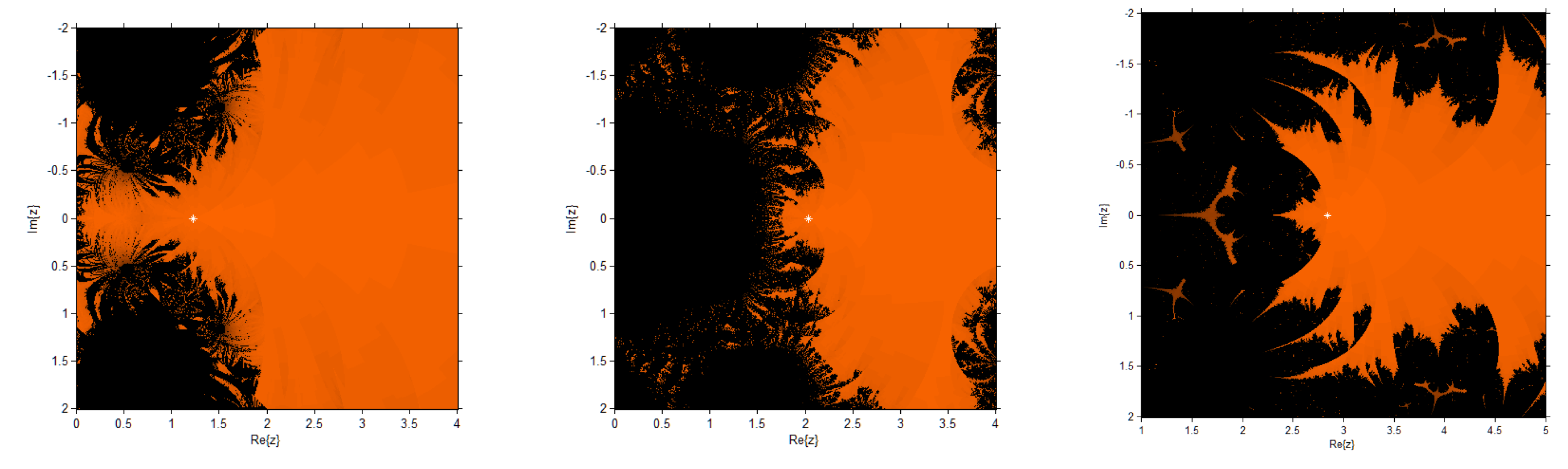
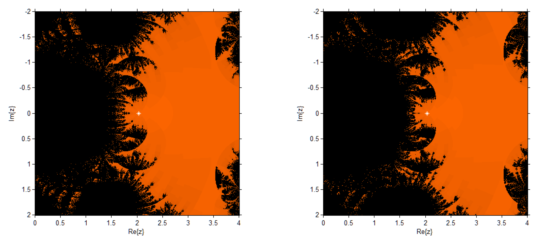
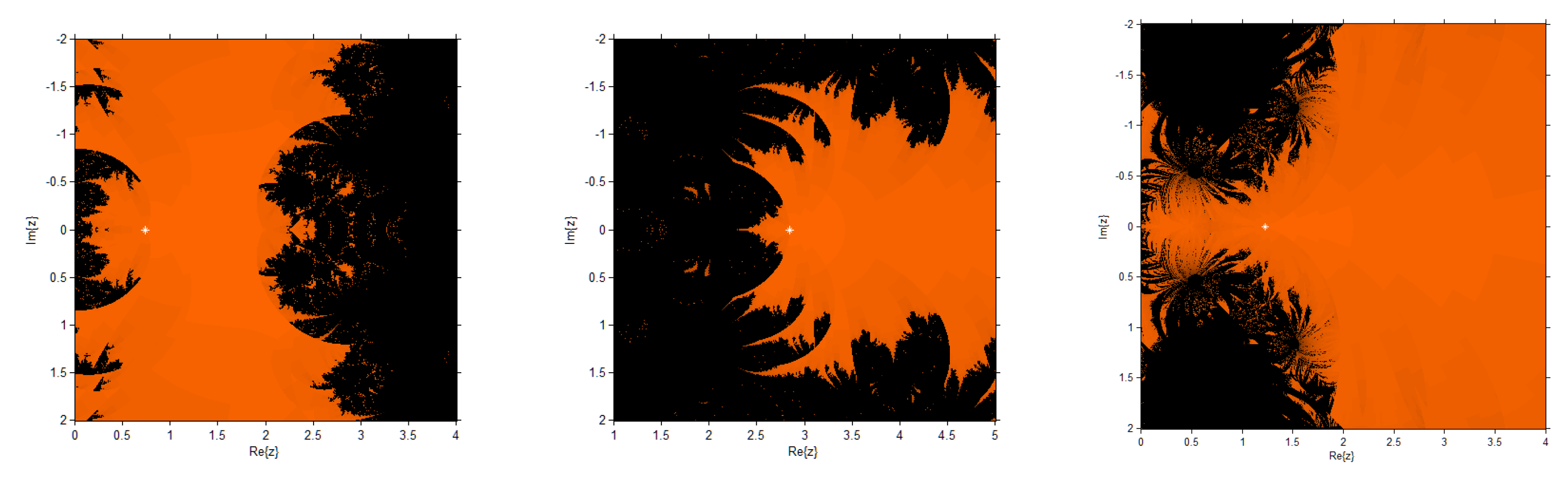
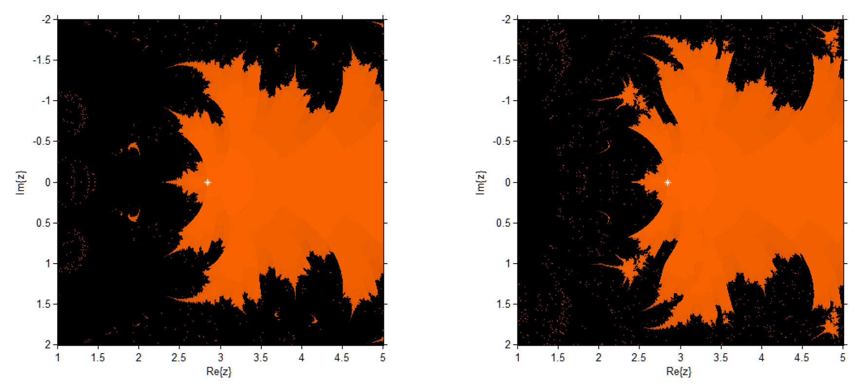
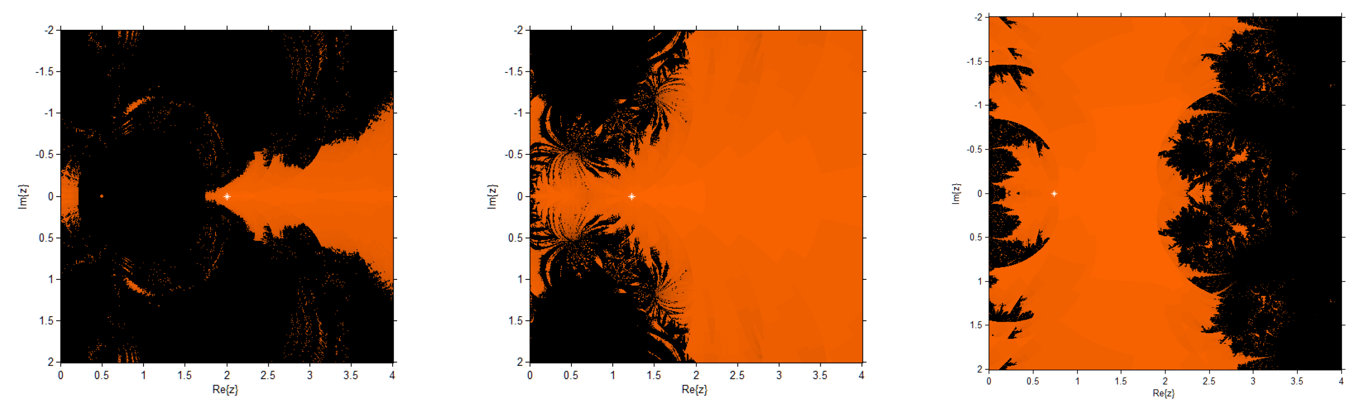
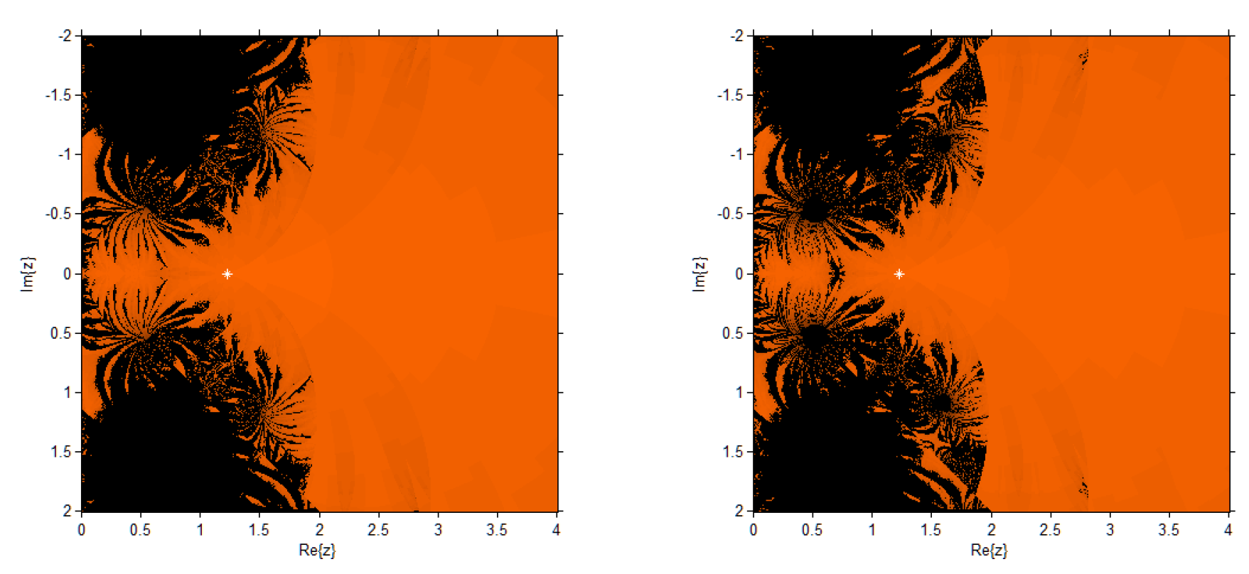
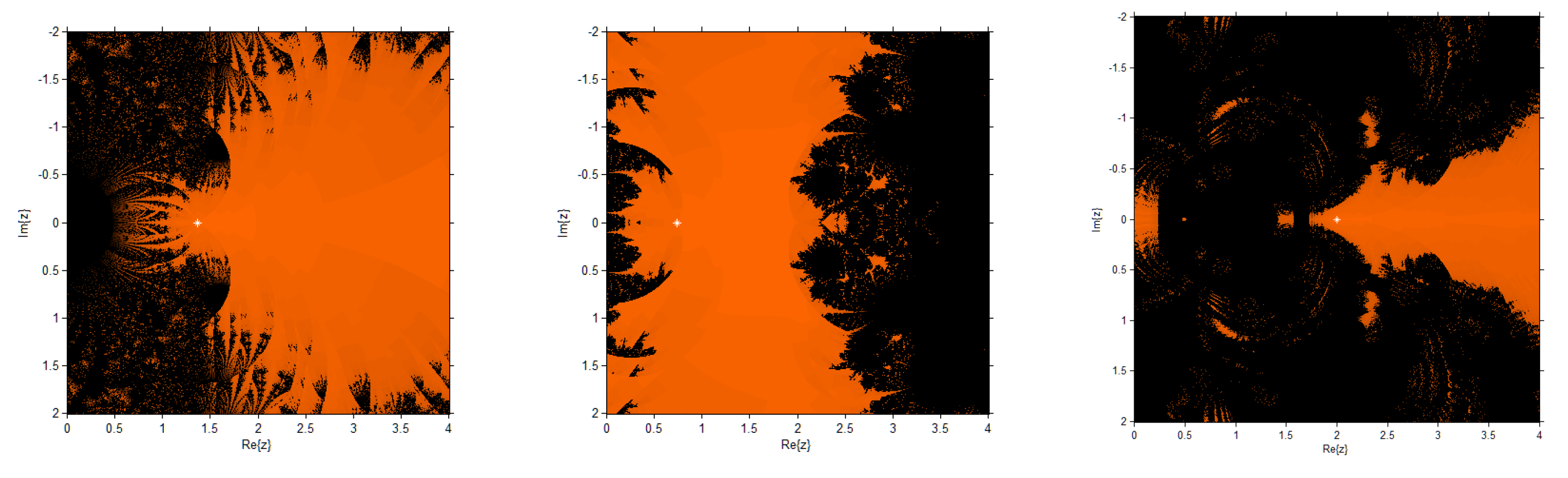
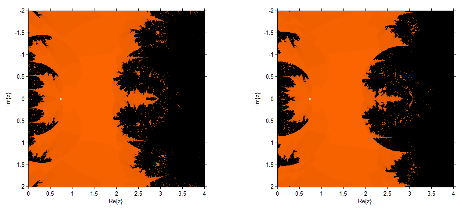
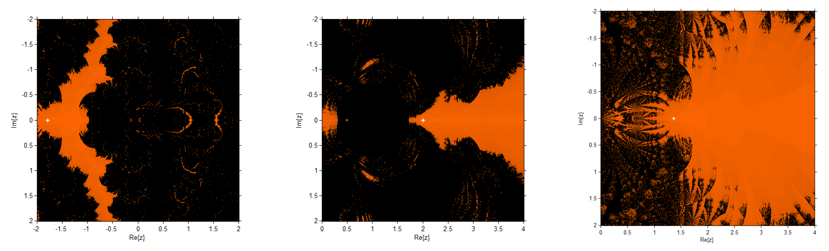
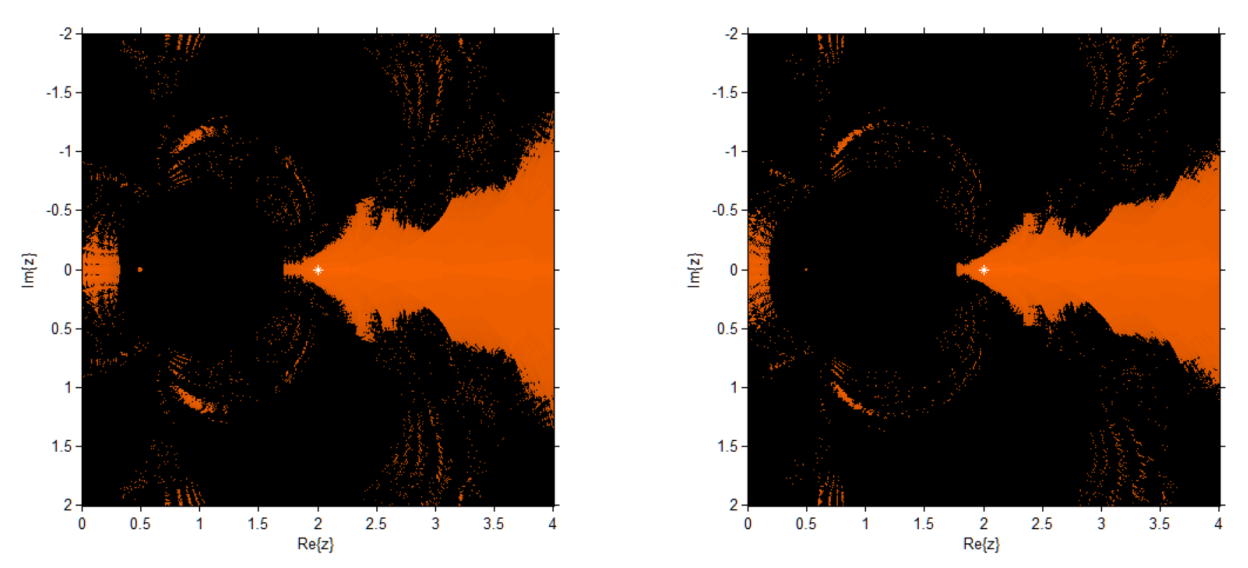
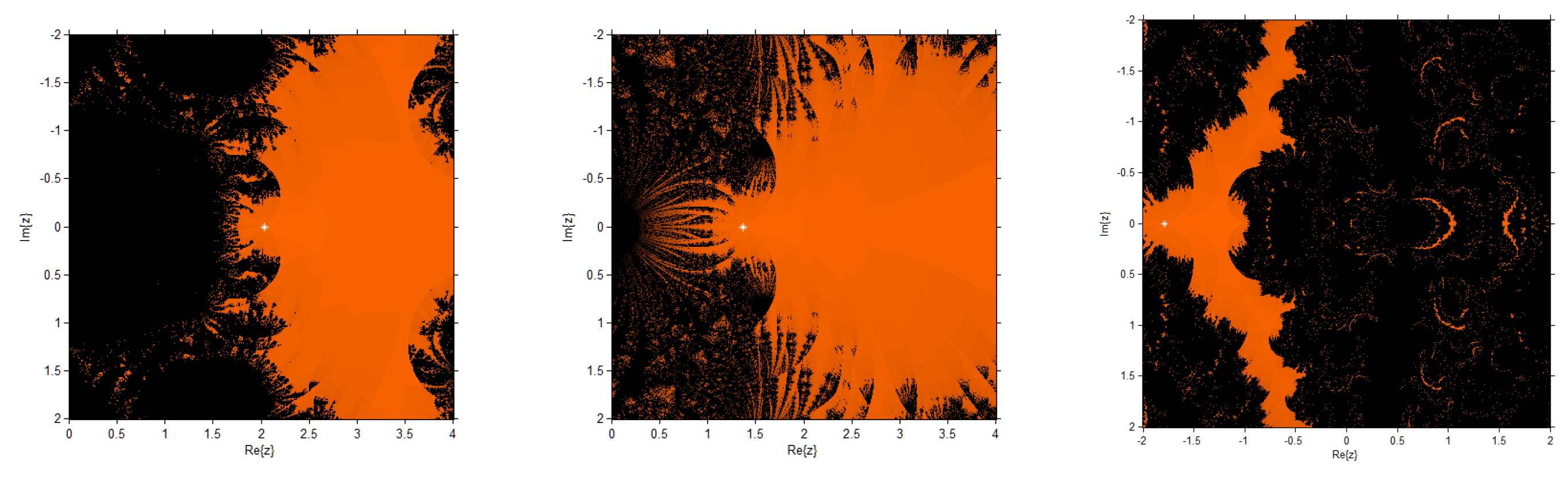
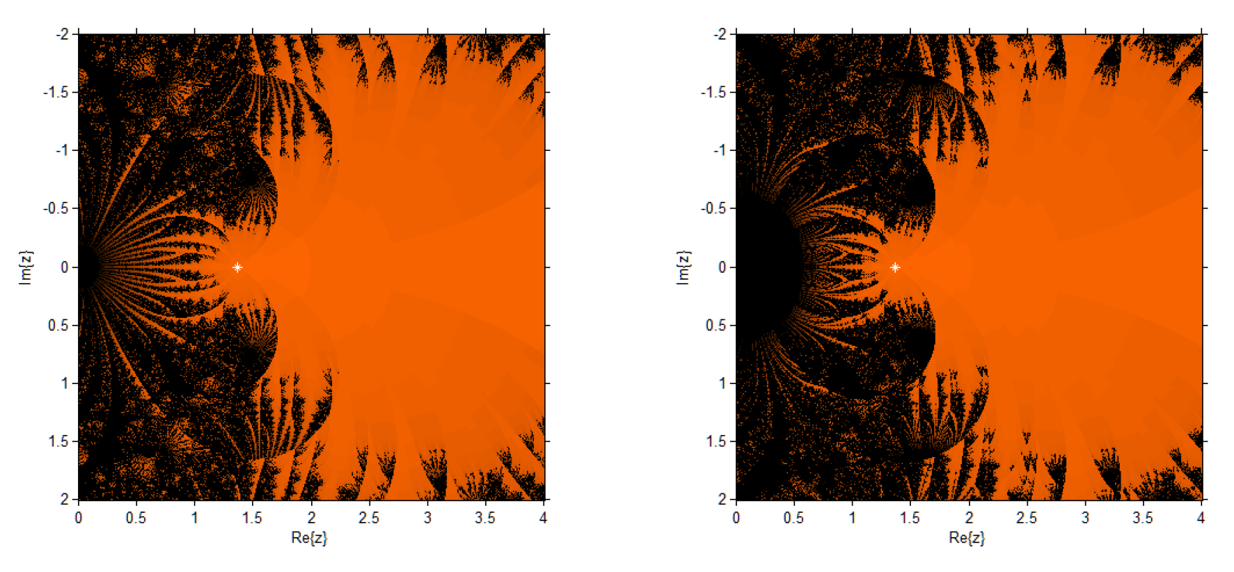
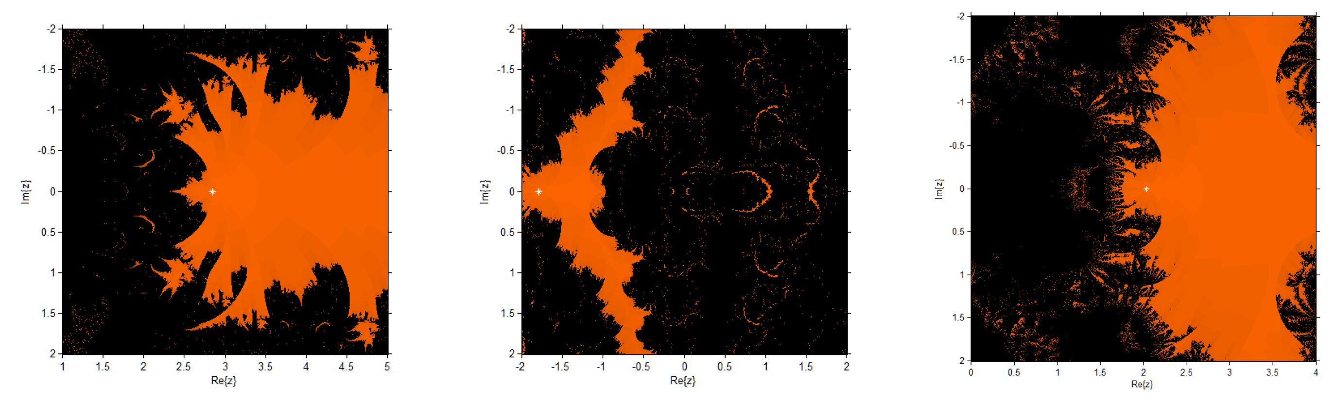
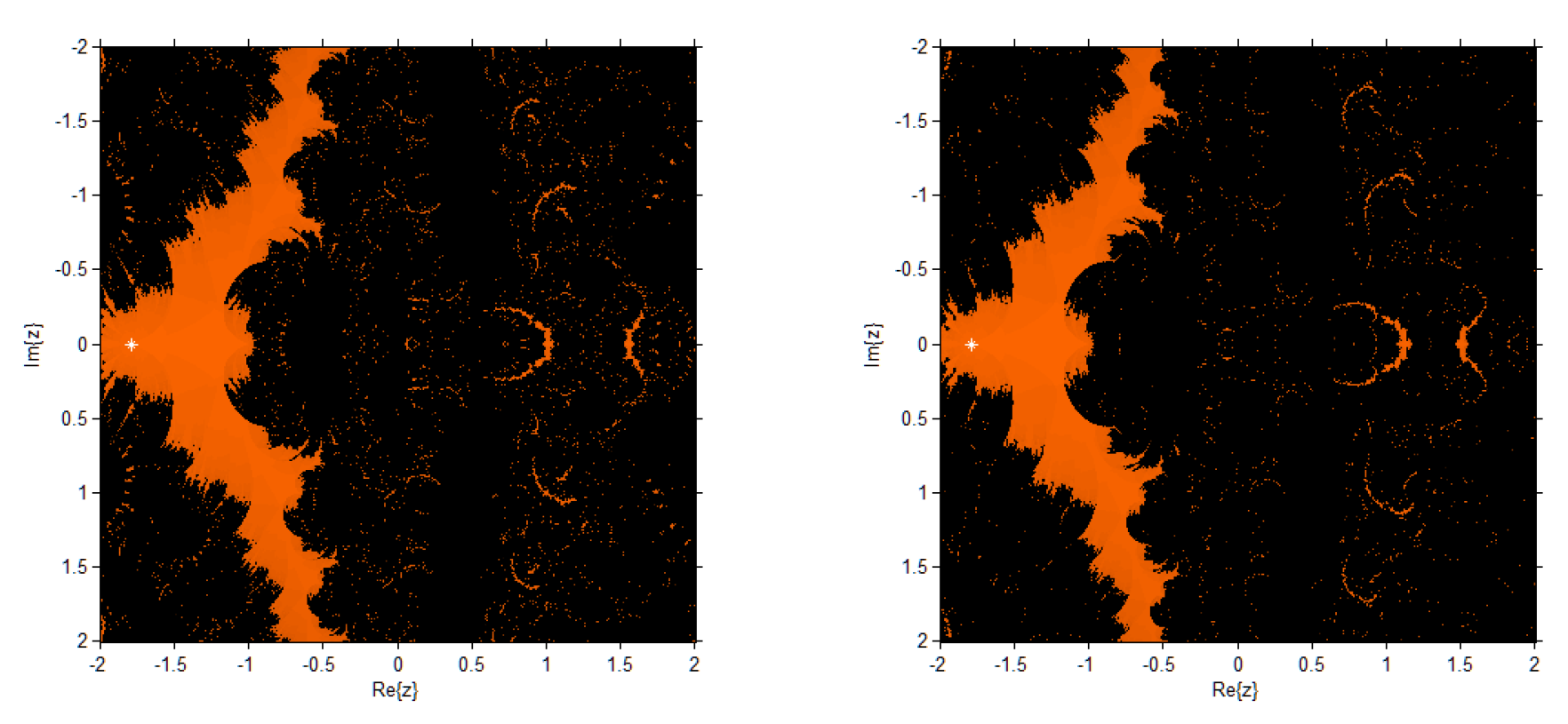
5. Dynamical Analysis

For the sake of stability comparison, we plot the dynamical planes corresponding to each scheme (SM-1, SM-2, SM-3, BM and ZM) for the nonlinear functions $f_1,f_2,f_3,f_4,f_5,f_6,f_7$ by using the procedure described in [24]. We draw a mesh of 400 × 400 points such that each point of the mesh is an initial-approximation of the required root of corresponding nonlinear function. The point is orange if the sequence of iteration method converges to the multiple root (with tolerance ${10}^{-3}$) in fewer than 80 iterations and the point is black if the sequence does not converges to the multiple root. The multiple zero is represented by a white star in the figures. Figure 1, Figure 2, Figure 3, Figure 4, Figure 5, Figure 6, Figure 7, Figure 8, Figure 9, Figure 10, Figure 11, Figure 12, Figure 13 and Figure 14 show that the basin of attraction drawn in orange is of the multiple zero only (i.e., a set of initial guesses converging to the multiple roots fills all the plotted regions of the complex plane). In general, convergence to other zeros or divergence can appear (referred to as strange stationary points). SM-1 has wider regions of convergence for $f_1$ as compared to ZM and BM in Figure 1 and Figure 2; SM-1 and SM-3 have wider regions of convergence for $f_2$ as compared to ZM and BM in Figure 3 and Figure 4. The convergence region of SM-2 for functions $f_3$, $f_4$ and $f_6$ is comparable with ZM and BM, as shown in Figure 5, Figure 6, Figure 7 and Figure 8, Figure 11 and Figure 12. For function $f_5$ in Figure 9 and Figure 10, the convergence region of SM-3 is better than ZM and BM. For function $f_7$, SM-1 and SM-3 have better convergence regions than ZM and BM, as shown in Figure 13 and Figure 14. Figure 1, Figure 2, Figure 3, Figure 4, Figure 5, Figure 6, Figure 7, Figure 8, Figure 9, Figure 10, Figure 11, Figure 12, Figure 13 and Figure 14 show that the region in orange is comparable or bigger for the presented methods SM-1, SM-2 and SM-3 than the regions obtained by schemes BM and ZM, which confirms the fast convergence and stability of the proposed schemes.

6. Conclusions

In this paper, we present a new family of optimal eighth-order schemes to find multiple roots of nonlinear equations. An extensive convergence analysis is done, which verifies that the new family is optimal eighth-order convergent. The presented family required four functional evaluations to get optimal eighth-order convergence, having efficiency index $8^{\frac{1}{4}}=1.6817$, which is higher than the efficiency index of the methods for multiple roots and of the families of Geum et al. [9,10]. Finally, numerical and dynamical tests confirmed the theoretical results and showed that the three members SM-1, SM-2 and SM-3 of the new family are better than existing methods for multiple roots. Hence, the proposed family is efficient among the domain of multiple root finding methods.

References

1. Ostrowski, A.M. Solution of Equations and Systems of Equations; Academic Press: New York, NY, USA, 1960. [Google Scholar]
2. Petkovic, M.S.; Neta, B.; Petkovic, L.D.; Dzunic, J. Multipoint Methods for Solving Nonlinear Equations; Academic Press: New York, NY, USA, 2013. [Google Scholar]
3. Traub, J.F. Iterative Methods for the Solution of Equations; Prentice-Hall: Englewood Cliffs, NJ, USA, 1964. [Google Scholar]
4. Schröder, E. Über unendlich viele algorithmen zur auflösung der gleichungen. Math. Annal. 1870, 2, 317–365. [Google Scholar] [CrossRef]
5. Singh, A.; Jaiswal, P. An efficient family of optimal fourth-order iterative methods for finding multiple roots of nonlinear equations. Proc. Natl. Acad. Sci. India Sec. A 2015, 85, 439–450. [Google Scholar] [CrossRef]
6. Behl, R.; Cordero, A.; Motsa, S.S.; Torregrosa, J.R.; Kanwar, V. An optimal fourth-order family of methods for multiple roots and its dynamics. Numer. Algorithms 2016, 71, 775–796. [Google Scholar] [CrossRef]
7. Biazar, J.; Ghanbari, B. A new third-order family of nonlinear solvers for multiple roots. Comput. Math. Appl. 2010, 59, 3315–3319. [Google Scholar] [CrossRef] [Green Version]
8. Chun, C.; Bae, H.J.; Neta, B. New families of nonlinear third-order solvers for finding multiple roots. Comput. Math. Appl. 2009, 57, 1574–1582. [Google Scholar] [CrossRef] [Green Version]
9. Geum, Y.H.; Kim, Y.I.; Neta, B. A class of two-point sixth-order multiple-zero finders of modified double-Newton type and their dynamics. Appl. Math. Comput. 2015, 270, 387–400. [Google Scholar] [CrossRef] [Green Version]
10. Geum, Y.H.; Kim, Y.I.; Neta, B. A sixth-order family of three-point modified Newton-like multiple-root finders and the dynamics behind their extraneous fixed points. Appl. Math. Comput. 2016, 283, 120–140. [Google Scholar] [CrossRef] [Green Version]
11. Hueso, J.L.; Martinez, E.; Treuel, C. Determination of multiple roots of nonlinear equation and applications. J. Math. Chem. 2015, 53, 880–892. [Google Scholar] [CrossRef]
12. Lee, S.; Choe, H. On fourth-order iterative methods for multiple roots of nonlinear equation with high efficiency. J. Comput. Anal. Appl. 2015, 18, 109–120. [Google Scholar]
13. Lin, R.I.; Ren, H.M.; Šmarda, Z.; Wu, Q.B.; Khan, Y.; Hu, J.L. New families of third-order iterative methods for finding multiple roots. J. Appl. Math. 2014, 2014. [Google Scholar] [CrossRef]
14. Li, S.; Cheng, L.; Neta, B. Some fourth-order nonlinear solvers with closed formulae for multiple roots. Comput. Math. Appl. 2010, 59, 126–135. [Google Scholar] [CrossRef] [Green Version]
15. Ahmad, N.; Singh, V.P. Some New Three step Iterative methods for solving nonlinear equation using Steffensen’s and Halley method. Br. J. Math. Comp. Sci. 2016, 19, 1–9. [Google Scholar] [CrossRef] [PubMed]
16. Neta, B. Extension of Murakami’s high-order non-linear solver to multiple roots. Int. J. Comput. Math. 2010, 87, 1023–1031. [Google Scholar] [CrossRef]
17. Sharma, J.R.; Sharma, R. Modified Jarratt method for computing multiple roots. Appl. Math. Comput. 2010, 217, 878–881. [Google Scholar] [CrossRef]
18. Zhou, X.; Chen, X.; Song, Y. Constructing higher-order methods for obtaining the multiple roots of nonlinear equations. J. Comput. Appl. Math. 2011, 235, 4199–4206. [Google Scholar] [CrossRef] [Green Version]
19. Kung, H.T.; Traub, J.F. Optimal order of one-point and multipoint iteration. J. Assoc. Comput. Mach. 1974, 21, 643–651. [Google Scholar] [CrossRef]
20. Behl, R.; Cordero, A.; Motsa, S.S.; Torregrosa, J.R. An eighth-order family of optimal multiple root finders and its dynamics. Numer. Algorithms 2018, 77, 1249–1272. [Google Scholar] [CrossRef]
21. Zafar, F.; Cordero, A.; Quratulain, R.; Torregrosa, J.R. Optimal iterative methods for finding multiple roots of nonlinear equations using free parameters. J. Math. Chem. 2017, 56, 1884–1901. [Google Scholar] [CrossRef] [Green Version]
22. Neta, B.; Chun, C.; Scott, M. On the development of iterative methods for multiple roots. Appl. Math. Comput. 2013, 224, 358–361. [Google Scholar] [CrossRef] [Green Version]
23. Weerakoon, S.; Fernando, T.G.I. A variant of Newton’s method with accelerated third-order convergence. Appl. Math. Lett. 2000, 13, 87–93. [Google Scholar] [CrossRef]
24. Chicharro, F.I.; Cordero, A.; Torregrosa, J.R. Drawing dynamical and pa- rameters planes of iterative families and methods. Sci. World J. 2013, 2013. [Google Scholar] [CrossRef] [PubMed]
Figure 1. Basins of attraction of SM1 (Left), SM2 (Middle) and SM3 (Right) for f 1 ( x ) .
Mathematics 07 00672 g001
Figure 2. Basins of attraction of BM (Left) and ZM (Right) for f 1 ( x ) .
Mathematics 07 00672 g002
Figure 3. Basins of attraction of SM1 (Left), SM2 (Middle) and SM3 (Right) for f 2 ( x ) .
Mathematics 07 00672 g003
Figure 4. Basins of attraction of BM (Left) and ZM (Right) for f 2 ( x ) .
Mathematics 07 00672 g004
Figure 5. Basins of attraction of SM1 (Left), SM2 (Middle) and SM3 (Right) for f 3 ( x ) .
Mathematics 07 00672 g005
Figure 6. Basins of attraction of BM (Left) and ZM (Right) for f 3 ( x ) .
Mathematics 07 00672 g006
Figure 7. Basins of attraction of SM1 (Left), SM2 (Middle) and SM3 (Right) for f 4 ( x ) .
Mathematics 07 00672 g007
Figure 8. Basins of attraction of BM (Left) and ZM (Right) for f 4 ( x ) .
Mathematics 07 00672 g008
Figure 9. Basins of attraction of SM1 (Left), SM2 (Middle) and SM3 (Right) for f 5 ( x ) .
Mathematics 07 00672 g009
Figure 10. Basins of attraction of BM (Left) and ZM (Right) for f 5 ( x ) .
Mathematics 07 00672 g010
Figure 11. Basins of attraction of SM1 (Left), SM2 (Middle) and SM3 (Right) for f 6 ( x ) .
Mathematics 07 00672 g011
Figure 12. Basins of attraction of BM (Left) and ZM (Right) for f 6 ( x ) .
Mathematics 07 00672 g012
Figure 13. Basins of attraction of SM1 (Left), SM2 (Middle) and SM3 (Right) for f 7 ( x ) .
Mathematics 07 00672 g013
Figure 14. Basins of attraction of BM (Left) and ZM (Right) for f 7 ( x ) .
Mathematics 07 00672 g014