On the Efficacy of Ensemble of Constraint Handling Techniques in Self-Adaptive Differential Evolution

Abstract

Self-adaptive variants of evolutionary algorithms (EAs) tune their parameters on the go by learning from the search history. Adaptive differential evolution with optional external archive (JADE) and self-adaptive differential evolution (SaDE) are two well-known self-adaptive versions of differential evolution (DE). They are both unconstrained search and optimization algorithms. However, if some constraint handling techniques (CHTs) are incorporated in their frameworks, then they can be used to solve constrained optimization problems (COPs). In an early work, an ensemble of constraint handling techniques (ECHT) is probabilistically hybridized with the basic version of DE. The ECHT consists of four different CHTs: superiority of feasible solutions, self-adaptive penalty, $\epsilon$-constraint handling technique and stochastic ranking. This paper employs ECHT in the selection schemes, where offspring competes with their parents for survival to the next generation, of JADE and SaDE. As a result, JADE-ECHT and SaDE-ECHT are developed, which are the constrained variants of JADE and SaDE. Both algorithms are tested on 24 COPs and the experimental results are collected and compared according to algorithms’ evaluation criteria of CEC’06. Their comparison, in terms of feasibility rate (FR) and success rate (SR), shows that SaDE-ECHT surpasses JADE-ECHT in terms of FR, while JADE-ECHT outperforms SaDE-ECHT in terms of SR.

1. Introduction

Evolutionary algorithms (EAs) are nature inspired population-based stochastic search and optimization methods. EAs work on the principle of natural evolution. In EAs, selected population members based on a fitness/selection scheme, the so called parents, undergo perturbation by applying genetic operators, mutation and crossover, to produce offspring. A selection scheme is then adopted to select the fittest individuals with a certain probability among the parents and offspring for the next generation. Many EAs, such as genetic algorithms (GAs), differential evolution (DE), particle swarm optimization (PSO), firefly algorithm (FA), bee algorithm (BA), ant colony optimization (ACO), evolution strategy (ES) etc. have been designed using different genetic operators and selection schemes for the unconstrained optimization problems since 1959.

Differential evolution (DE) [1] has proven to be a simple and efficient EA for many optimization problems. A number of variants of DE were developed and are in practice for unconstrained/constrained optimization [2,3,4,5,6,7,8,9]. In DE, a random initial population of size $NP$ is generated in the whole search space to a possible extent and the fittest/best with minimum function value in the initial population is found. It then invokes one of the different mutation strategies such as DE/rand/1, DE/current to best/2, DE/rand/2, DE/current-to-rand/1 to generate a mutant vector. For example in DE/rand/1, the weighted difference scaled by a scaling factor $F\in [0,2]$ between two population vectors is added to a target vector to generate a mutant vector. Afterwards, the parameters of mutant vector and target vector are mixed with a certain crossover probability $C_r\in [0,1]$ to produce the trial vector. Using the one-to-one-spawning selection mechanism, if the objective function value of the trial vector is less than the objective function value of the target vector, in minimization sense, then the trial vector replaces the target vector and becomes the parent for the next generation. The three steps of producing the mutant vector, the trail vector and comparison of the target and trial vectors are repeated until a stopping criterion is met. Also, the fittest/best individual is updated after every generation by comparing the function values of the trial vector, if it is successful in selection process, and fittest/best individual found so far. For more details of DE and different mutation strategies used in it, the readers are referred to [10,11].

The performance of the original DE algorithm is highly dependent on the mutation strategies and its parameters’ settings [11,12,13,14]. During different evolution stages, different strategies and different parameters’ settings with different global and local search capabilities might be preferred. Huang et al. developed a self-adaptive DE variant, SaDE [10]. SaDE automatically adapts the learning strategies and the parameters’ settings during evolution. It probabilistically selects one of the four mutation strategies: DE/rand/1, DE/current to best/2, DE/rand/2, DE/current-to-rand/1 for each individual in the current population. J. Zhang and A. C. Sanderson developed another self-adaptive DE version, self-adaptive differential evolution with optional external archive (JADE) [15]. JADE too automates the parameters and employs the mutation strategy DE/current-to-pbest with the optional external archive. The strategy DE/current-to-pbest uses not only the information of the best solution, but also the information on the other good solutions. The external archive keeps record of the inferior solutions, which are then used for diversity among population members and avoiding premature convergence.

For recent advances in DE, the readers are referred to [16,17]. EAs suit a variety of applications in the fields of engineering and science [18,19,20,21,22,23,24]. Generally, EAs outperform traditional optimization algorithms for problems which are not continuous, non-differentiable, multi-modal, noisy and not well-defined. However, EAs are unconstrained optimization techniques. They are not capable to directly solve COPs having constraints of any kind (e.g., equality, inequality, linear and non-linear etc.). To overcome this problem, CHTs are used with EAs to handle all types of constraints. The last three decades have witnessed many techniques for handling constraints by EAs [20,25]. Michalewicz and Schoenauer [26] categorized them into five classes: preserving feasibility of solutions, adopting penalty functions, separating feasible solutions from infeasible ones, decoding, and hybridizing different techniques. However, according to no free lunch theorem (NFL) [27], a single CHT can not outperform all other CHTs on each problem. Same is true for different EAs as well. Thus, one has to try and combine different CHTs and EAs to design a suitable algorithm that can solve most of the problems. So keeping in mind the NFL theorem and some other individual problems of COPs, an ensemble of constraint handling techniques (ECHT) is combined with the basic version of DE in [28,29]. ECHT consists of four different CHTs: superiority of feasible solutions, self-adaptive penalty, $\epsilon$-constraint handling technique and stochastic ranking. SaDE and JADE, being advanced self-adaptive variants, are both unconstrained search and optimization algorithms. Like other EAs, they also need some additional CHTs to solve constrained optimization problems (COPs).

In this work, the ECHT is implemented in the selection scheme, where offspring and parents compete for survival to next generation, of JADE and SaDE. As a result, constrained versions of JADE and SaDE, denoted by JADE-ECHT and SaDE-ECHT, are developed. The performance of JADE-ECHT and SaDE-ECHT is tested and compared based on feasibility rate (FR) and success rate (SR) on 24 COPs according to algorithms’ evaluation criteria of CEC’06.

This rest of this paper is ordered as follows. The general COP and ECHT are detailed in Section 2. Section 3 presents the proposed modified algorithms, JADE-ECHT and SaDE-ECHT. Section 4 presents and discusses the experimental results obtained with JADE-ECHT and SaDE-ECHT. Finally, Section 5 describes the concluding remarks of this work.

2. Constrained Optimization Problem and ECHT

This section first describes the constrained optimization problem to be considered in this work. It then illustrates the four CHTs of ECHT.

2.1. Constrained Optimization Problem (COP)

Time, physical, and geometric etc. type constraints exist in most of the real world optimization problems. Such problems can be modelled as a COP. Mathematically, a COP, in case of minimization, can be formulated as follows [30]:

$$\begin{array}{c}\mathrm{Minimize}f\left(\mathbf{x}\right),\mathbf{x}={[x_1,x_2,\dots ,x_n]}^T\hfill \\ \mathrm{subject}\mathrm{to}\hfill \\ g_i\left(\mathbf{x}\right)\le 0i=1,\dots ,l,\hfill \\ h_j\left(\mathbf{x}\right)=0j=l+1,\dots ,p,\hfill \\ l_i\le x_i\le u_i,i=1,2,\dots ,n.\hfill \end{array}$$

(1)

In problem (1), $f\left(\mathbf{x}\right)$ is called cost function which will be minimized. In case of maximizing the cost function, it needs to be multiplied with a negative sign. The n-dimensional vector $\mathbf{x}$ is called decision variable vector. There are l inequality and $p-l$ equality constraints. An inequality constraint $g_j\left(\mathbf{x}\right)$ becomes an active constraint, if $g_j\left({\mathbf{x}}^{*}\right)=0$, where ${\mathbf{x}}^{*}$ is global optimum solution, whereas equality constraints, $h_j\left(\mathbf{x}\right)=0$, are active by default. Generally, equality constraints are converted into inequality constraints by $|h_j\left(\mathbf{x}\right)|-ϵ\le 0$, where $ϵ$ is an acceptable tolerance for equality constraints. According to CEC’06 [30] evaluation criteria, $ϵ$ is set to 0.0001 (in this work, we will also use the same value for $ϵ$ ). $l_i$ and $u_i$ are the lower and upper bounds of component $x_i$ of vector $\mathbf{x}$. They form the whole search space S. The solution $\mathbf{x}\in S$ is referred to be feasible, if it satisfies all the equality and inequality constraints of problem (1); otherwise, it is called infeasible. We denote with F the set of all feasible solutions and normally $F\subset S$. The total constraints’ violation for an infeasible solution is defined as [28,29]:

$$v\left(\mathbf{x}\right)=\frac{{\sum }_{i=1}^p{c}_i\left(g_i^{\prime }\left(\mathbf{x}\right)\right)}{{\sum }_{i=1}^p{c}_i},$$

(2)

where

$$\begin{array}{c}\hfill g_i^{\prime }\left(\mathbf{x}\right)=\left\{\begin{array}{cc}max\{g_i\left(\mathbf{x}\right),0\},\hfill & i=1,\dots ,l\hfill \\ max\left\{\right|h_j\left(\mathbf{x}\right)|-ϵ,0\},\hfill & j=l+1,\dots ,p.\hfill \end{array}\right.,\end{array}$$

(3)

where $c_i(=1/g_{ma{x}_i}^{\prime })$ denotes weight parameter, $g_{ma{x}_i}^{\prime }$ denotes the maximum constraint violation of constraint $g_i\left(\mathbf{x}\right),i=1,\dots ,l$ obtained thus far. It maybe noted that $c_i$ changes during the evolution process. This helps in balancing how each constraint contributes in the problem irrespective of their different numerical ranges. The four constraints handling techniques which are used in this work are detailed as follows.

2.2. Superiority of Feasible Solutions (SF)

As the name suggests, in SF feasible solutions have priority over infeasible solutions. SF was first suggested by Deb [31]. In this method, two solutions, a parent ${\mathbf{x}}^i$ and an offspring ${\mathbf{x}}^j$ compete. The parent ${\mathbf{x}}^i$ is considered better than the offspring ${\mathbf{x}}^j$, if any of the subsequent three settings is met [31]:

• Parent, ${\mathbf{x}}^i$ is feasible and offspring, ${\mathbf{x}}^j$ is infeasible.
• Both parent and offspring, ${\mathbf{x}}^i$ and ${\mathbf{x}}^j$ are feasible, but parent, ${\mathbf{x}}^i$ has minimum fitness value than the offspring, ${\mathbf{x}}^j$.
• Both ${\mathbf{x}}^i$ and ${\mathbf{x}}^j$ are infeasible, and overall constraints’ violation $v\left({\mathbf{x}}^i\right)$ of parent, ${\mathbf{x}}^i$ is less than overall constraints’ violation $v\left({\mathbf{x}}^j\right)$ of offspring, ${\mathbf{x}}^j$, where $v\left({\mathbf{x}}^i\right)$ and $v\left({\mathbf{x}}^j\right)$ are calculated by using Equation (2).

2.3. Self-Adaptive Penalty (SP)

Penalty methods are the most common approaches to handle constraints in the family of CHTs. In these techniques, in order to penalize an infeasible solution, the cost value of each infeasible solution and a penalty term corresponding to its constraints’ violation are added, in minimization sense (subtracted in maximization sense). In SP [28], an attempt has been made to facilitate the algorithm to search for feasible solutions, in case there are few feasible solutions, and find the optimum, in case there are enough feasible solutions. For this purpose, two penalties are added to the cost of an infeasible solution. This help in identifying the best infeasible solutions in the existing population. The amount of the added penalties considers the number of feasible solutions that exist in the current population. Thus, if there are few feasible solutions in the combined population of parents and offspring, the amount of penalty to infeasible individuals with higher constraints’ violation will be greater. On the contrary, with many feasible solutions, the fittest infeasible solutions in terms of cost are less penalized.

2.4. The $\epsilon$-Constraint (EC) Handling Technique

The $\epsilon$-constraint (EC) handling technique [32] adopts the parameter $\epsilon$ to relax the active constraints. The parameter $\epsilon$ is updated until a fixed generation counter is reached. Afterwards, $\epsilon$ becomes 0 to get individuals with no constraints’ violation (for detailed formulation of this technique, please see [28,32]).

2.5. Stochastic Ranking (SR)

SR [33] stochastically balances overall constraints’ violation and fitness function value. A solution is ranked based on its cost value, if it is feasible or if a randomly generated number is smaller than a probability factor $p_f$; otherwise, it is ranked on the constraints’ violation. The proposed value of $p_f=0.475$. However, if this constant value is not used, then it decreases linearly from $p_f=0.475$ to $p_f=0.025$ from initial generation to the last generation.

In [28], the ECHT is tested with evolutionary programming (EP) and basic DE. In this paper, we hybridize ECHT with the advanced versions of DE, JADE [15] and SaDE [10].

3. JADE-ECHT and SaDE-ECHT

In this section, we first give the algorithmic details of JADE-ECHT, which is then followed by the details of SaDE-ECHT.

3.1. JADE-ECHT

JADE [15] is an updated version of DE. It is also an unconstrained optimization algorithm. So it needs some additional CHTs to solve COPs. In this work, we embed the four above discussed CHTs in the selection scheme of JADE to modify it for solving COPs. The whole procedure of the proposed technique JADE-ECHT, shown in Figure 1, is discussed as follows.

Step 1:

generate initial population P, set the generation number $t=1$, initial crossover probability ${\mu }_{CR}=0.5$, initial mutation factor ${\mu }_F=0.5$, the set of archive inferior solutions $A_i=\varnothing$, the sets of successful mutation factors and crossovers, $S_F^i=\varnothing$, $S_{CR}^i=\varnothing$, respectively, where $i=1,\dots ,4$.

Step 2:

divide population P into four subpopulations, $P_i,i=1,\dots ,4$ each of size $PS$ (population size to be tackled by each CHT). Set parameters ${PAR}_i$, $i=1,\dots ,4$ of $PS$ individuals each with dimension D according to the rules of JADE and corresponding CHT. Also, calculate $F_l^i$ and $C{R}_l^i,\forall l\in \{1,\dots ,PS\}$, where $C{R}_l^i=rand{n}_l^i({\mu }_{CR},0.1)$, $F_l^i=rand{n}_l^i({\mu }_{CR},0.1)$.

Step 3:

compute the cost and the total constraints’ violation for every solution in each subpopulation using Equations (1)–(3).

Step 4:

each parent subpopulation $(P_i,i=1,\dots ,4)$ generates offspring subpopulation $(OF{F}_i,i=1,\dots ,4)$ as a result of applying mutation and crossover operators, respectively as follows [15]:

$${\mathbf{v}}_{l,t}^i={\mathbf{x}}_{l,t}^i+F_l^i\cdot ({\mathbf{x}}_{pbest,t}^i-{\mathbf{x}}_{l,t}^i)+F_l^i\cdot ({\mathbf{x}}_{r_1^l,t}^i-{\tilde{\mathbf{x}}}_{r_2^l,t}^i),$$

where ${\mathbf{x}}_{pbest,t}$ is one of the $100P\%$ best vectors. and ${\tilde{\mathbf{x}}}_{r_2^l,t}^i\ne {\mathbf{x}}_{r_1^l,t}^i\ne {\mathbf{x}}_{l,t}^i$ are chosen randomly from the existing population, P and from the union of current population and archived population, $P\cup A$. The archive A retains the parent individuals that are unsuccessful in the selection scheme.

$$\begin{array}{c}\hfill u_{l,t}^i=\left\{\begin{array}{cc}{v}_{l,t}^i,\hfill & \mathrm{if}(ran{d}_j[0,1]<{\mu }_{CR}or(j=j_{rand})\hfill \\ x_{l,t}^i,\hfill & \mathrm{otherwise}.\hfill \end{array}\right.\end{array}$$

(4)

In Equation (4), $v_{l,t}^i$ and $x_{l,t}^i$ are the $l\mathrm{th}$ components of the $i$ mutant and trial vectors in generation t.

Step 5:

evaluate the cost and the total constraints’ violation for every offspring in each subpopulation using Equations (1)–(3). Every offspring holds the cost and constraints values distinctly.

Step 6:

each parent subpopulation is grouped together with its own offspring and the offspring produced by the remaining three subpopulations corresponding to different CHTs. This way four different groups of populations are generated.

Step 7:

Parents population P for the next generation is selected from the four groups according to the rule of each CHT. Unsuccessful parents are added to the archive $A_i$. All successful crossover probabilities from $C{R}_{PS}^i$ and mutation factors from $F_{PS}^i$ are added to $S_{CR}^i$ and $S_F^i$.

Step 8:

Remove solutions randomly from $A_i$ so that $|A_i|\le PS$. Update ${\mu }_{CR}$ and ${\mu }_F$ adopting the formulations of [28].

Step 9:

If the stopping criteria are not met, go to Step 2; otherwise, stop.

3.2. SaDE-ECHT

SaDE [10] is also an unconstrained optimization algorithm. Like JADE and other EAs, it also needs some additional mechanisms to solve COPs. In this work, the four CHTs of ECHT are used in the selection scheme of SaDE for solving COPs. The whole procedure of proposed SaDE-ECHT, shown in Figure 2, is as follow:

Step 1:

generate initial population P, initiate the generation counter $t=1$, initial crossover probability ${\mu }_{CR}=0.5$, initial mutation factor ${\mu }_F=0.5$.

Step 2:

divide population P into four subpopulations, $P_i,i=1,\dots ,4$ each of size $PS$. Set parameters ${PAR}_i$, where $i=1,\dots ,4$ of $PS$ individuals each with dimension D and generate F in [0,2] and $CR$ in (0,1) by using normal distribution according to the rules of SaDE and corresponding CHT.

Step 3:

compute the cost and the total constraints’ violation for every solution in each subpopulation using Equations (1)–(3).

Step 4:

each parent in each subpopulation produces offspring by using one of the four mutation strategies, DE/rand/1, DE/current-to-best/2, DE/rand/2, and DE/current-to-rand/1 (for details of these strategies, please see [10]) and crossover given in Equation (4). For first 20 generations, probabilities are fixed and set to $p_1=p_2=p_3=p_4=0.25$. Afterwards, the Roulette Wheel selection is adopted to update the respective probability $p_i$ as follows [10]:

$$p_i=\frac{n{s}_i}{n{s}_i+n{f}_i},i=1,2,3,4$$

(5)

Step 5:

evaluate the cost and the total constraints’ violation for every offspring in each subpopulation using Equations (1)–(3).

Step 6:

each parent subpopulation is grouped together with its own offspring and the offspring produced by the remaining three subpopulations corresponding to different CHTs. This way four different groups of populations are generated.

Step 7:

parents population P for the next generation are selected from the four groups according to the rule of each CHT.

Step 8:

recalculate crossover probability after every five generations according to the mean of recorded $CR$ values.

Step 9:

if the stopping criteria are not met, go to Step 2; otherwise, stop.

4. Experimental Results

The performances of JADE-ECHT and SaDE-ECHT were evaluated on the suit of CEC’06, which contains twenty four benchmark functions. The PC configuration and parameters’ settings are given in

Table 1. Configuration of the PC.

System	Windows 8
CPU	3.00 GHz
Ram	2 GB
Language	MATLAB 2012, 8.0.0.783

and

Table 2. Parameters’ settings.

Parameters’ Description	Parameters’ Settings
Population size for each CHT	$PS=25$
Whole population size	$NP=4\ast PS=100$
Maximum number of generations	$t=2500$
Total number of runs	$runs=25$
Initial value of mutation factor	${\mu }_F=0.5$
Initial value of crossover probability	${\mu }_{CR}=0.5$
Termination criterion based on maximum function evaluations	$max\_FEs=\mathrm{500,000}$.

.

Result Achieved

In

Table 3. Comparison of self-adaptive differential evolution with optional external archive (JADE)-ensemble of constraint handling techniques (ECHT) and self-adaptive differential evolution (SaDE)-ECHT after FES = 500,000 for g01–g06. The bold numbers indicate the better results.

Prob	Algorithm	Best	Median	Worst	c	$\overline{\mathit{v}}$	Mean	Std	FR	SR
$\mathrm{g}01$	JADE-ECHT	$0\left(0\right)$	$0\left(0\right)$	$2.0000\left(0\right)$	$0,0,0$	0	$0.0800$	$0.4000$	$100\%$	$96\%$
	SaDE-ECHT	$0\left(0\right)$	$0\left(0\right)$	$\mathbf{0}\left(\mathbf{0}\right)$	$0,0,0$	0	$\mathbf{0}$	$\mathbf{0}$	$100\%$	100%
$\mathrm{g}02$	JADE-ECHT	$0.0001\left(0\right)$	$\mathbf{0.0004}\left(\mathbf{0}\right)$	$\mathbf{0.0276}\left(\mathbf{0}\right)$	$0,0,0$	0	$\mathbf{0.0064}$	$\mathbf{0.0091}$	$100\%$	$16\%$
	SaDE-ECHT	$\mathbf{0}\left(\mathbf{0}\right)$	$0.0110\left(0\right)$	$0.1263\left(0\right)$	$0,0,0$	0	$0.0191$	$0.0254$	$100\%$	24%
$\mathrm{g}03$	JADE-ECHT	$0.0250\left(0\right)$	$0.1015\left(0\right)$	$0.4245\left(0\right)$	$0,0,0$	0	$0.1385$	$0.1036$	$100\%$	$0\%$
	SaDE-ECHT	$\mathbf{0}\left(\mathbf{0}\right)$	$\mathbf{0.0122}\left(\mathbf{0}\right)$	$\mathbf{0.1524}\left(\mathbf{0}\right)$	$0,0,0$	0	$\mathbf{0.0243}$	$\mathbf{0.0343}$	$100\%$	12%
$\mathrm{g}04$	JADE-ECHT	$0\left(0\right)$	$0\left(0\right)$	$0\left(0\right)$	$0,0,0$	0	0	0	$100\%$	$100\%$
	SaDE-ECHT	$0\left(0\right)$	$0\left(0\right)$	$0\left(0\right)$	$0,0,0$	0	0	0	$100\%$	$100\%$
$\mathrm{g}05$	JADE-ECHT	$0\left(0\right)$	$\mathbf{0}\left(\mathbf{0}\right)$	$\mathbf{0}\left(\mathbf{0}\right)$	$0,0,0$	0	$\mathbf{0}$	$\mathbf{0}$	$100\%$	100%
	SaDE-ECHT	$0\left(0\right)$	$91.4773\left(0\right)$	$515.4900\left(0\right)$	$0,0,0$	0	$110.1546$	$101.2496$	$100\%$	$4\%$
$\mathrm{g}06$	JADE-ECHT	$0\left(0\right)$	$0\left(0\right)$	$0\left(0\right)$	$0,0,0$	0	0	0	$100\%$	$100\%$
	SaDE-ECHT	$0\left(0\right)$	$0\left(0\right)$	$0\left(0\right)$	$0,0,0$	0	0	0	$100\%$	$100\%$

,

Table 4. Comparison of JADE-ECHT and SaDE-ECHT after FES = 500,000 for g07–g12. The bold numbers indicate the better results.

Prob	Algorithm	Best	Median	Worst	c	$\overline{\mathit{v}}$	Mean	Std	FR	SR
$\mathrm{g}07$	JADE-ECHT	$\mathbf{0}\left(\mathbf{0}\right)$	$0.0879\left(0\right)$	$\mathbf{0.2651}\left(\mathbf{0}\right)$	$0,0,0$	0	$0.0976$	$\mathbf{0.0726}$	$100\%$	4%
	SaDE-ECHT	$0.0001\left(0\right)$	$\mathbf{0.0114}\left(\mathbf{0}\right)$	$0.3230\left(0\right)$	$0,0,0$	0	$\mathbf{0.0518}$	$0.0850$	$100\%$	$0\%$
$\mathrm{g}08$	JADE-ECHT	$0\left(0\right)$	$0\left(0\right)$	$0\left(0\right)$	$0,0,0$	0	0	0	$100\%$	$100\%$
	SaDE-ECHT	$0\left(0\right)$	$0\left(0\right)$	$0\left(0\right)$	$0,0,0$	0	0	0	$100\%$	$100\%$
$\mathrm{g}09$	JADE-ECHT	$0\left(0\right)$	$0.0039\left(0\right)$	$0.0714\left(0\right)$	$0,0,0$	0	$0.0132$	$0.0192$	$100\%$	$20\%$
	SaDE-ECHT	$0\left(0\right)$	$\mathbf{0}\left(\mathbf{0}\right)$	$\mathbf{0.0006}\left(\mathbf{0}\right)$	$0,0,0$	0	$\mathbf{0.0001}$	$\mathbf{0.0002}$	$100\%$	76%
$\mathrm{g}10$	JADE-ECHT	$\mathbf{0}\left(\mathbf{0}\right)$	$133.9677\left(0\right)$	$343.5425\left(0\right)$	$0,0,0$	0	$143.0809$	$105.4501$	$100\%$	4%
	SaDE-ECHT	$0.0012\left(0\right)$	$\mathbf{0.1709}\left(\mathbf{0}\right)$	$\mathbf{11.9004}\left(\mathbf{0}\right)$	$0,0,0$	0	$\mathbf{1.1748}$	$\mathbf{3.0352}$	$100\%$	$0\%$
$\mathrm{g}11$	JADE-ECHT	$0\left(0\right)$	$0\left(0\right)$	$0\left(0\right)$	$0,0,0$	0	0	0	$100\%$	$100\%$
	SaDE-ECHT	$0\left(0\right)$	$0\left(0\right)$	$0\left(0\right)$	$0,0,0$	0	0	0	$100\%$	$100\%$
$\mathrm{g}12$	JADE-ECHT	$0\left(0\right)$	$0\left(0\right)$	$0\left(0\right)$	$0,0,0$	0	0	0	$100\%$	$100\%$
	SaDE-ECHT	$0\left(0\right)$	$0\left(0\right)$	$0\left(0\right)$	$0,0,0$	0	0	0	$100\%$	$100\%$

,

Table 5. Comparison of JADE-ECHT and SaDE-ECHT after FES = 500,000 for g13–g18. The bold numbers indicate the better results.

Prob	Algorithm	Best	Median	Worst	c	$\overline{\mathit{v}}$	Mean	Std	FR	SR
$\mathrm{g}13$	JADE-ECHT	$0.3849\left(0\right)$	$0.9118\left(0\right)$	$0.9459\left(0\right)$	$0,0,0$	0	$0.8275$	$\mathbf{0.1750}$	$100\%$	$0\%$
	SaDE-ECHT	$\mathbf{0}\left(\mathbf{0}\right)$	$\mathbf{0.3870}\left(\mathbf{0}\right)$	$\mathbf{0.8491}\left(\mathbf{0}\right)$	$0,0,0$	0	$\mathbf{0.3608}$	$0.2828$	$100\%$	4%
$\mathrm{g}14$	JADE-ECHT	$\mathbf{0}\left(\mathbf{0}\right)$	$\mathbf{0.0174}\left(\mathbf{0}\right)$	$5.5402\left(0\right)$	$0,0,0$	0	$1.9415$	$2.2940$	$100\%$	40%
	SaDE-ECHT	$0.4527\left(0\right)$	$1.6397\left(0\right)$	$\mathbf{3.3912}\left(\mathbf{0}\right)$	$0,0,0$	0	$\mathbf{1.7600}$	$\mathbf{0.6956}$	$100\%$	$0\%$
$\mathrm{g}15$	JADE-ECHT	$0\left(0\right)$	$\mathbf{0}\left(\mathbf{0}\right)$	$\mathbf{0}\left(\mathbf{0}\right)$	$0,0,0$	0	$\mathbf{0}$	$\mathbf{0}$	$100\%$	100%
	SaDE-ECHT	$0\left(0\right)$	$0.0009\left(0\right)$	$2.5449\left(0\right)$	$0,0,0$	0	$0.3333$	$0.6971$	$100\%$	$44\%$
$\mathrm{g}16$	JADE-ECHT	$0\left(0\right)$	$0\left(0\right)$	$0\left(0\right)$	$0,0,0$	0	0	0	$100\%$	$100\%$
	SaDE-ECHT	$0\left(0\right)$	$0\left(0\right)$	$0\left(0\right)$	$0,0,0$	0	0	0	$100\%$	$100\%$
$\mathrm{g}17$	JADE-ECHT	$\mathbf{0}\left(\mathbf{0}\right)$	$\mathbf{0}\left(\mathbf{0}\right)$	$\mathbf{74.0580}\left(\mathbf{0}\right)$	$0,0,0$	0	$\mathbf{8.8870}$	$\mathbf{24.5623}$	$100\%$	88%
	SaDE-ECHT	$7.9251\left(0\right)$	$91.2351\left(0\right)$	$297.1687\left(0\right)$	$0,0,0$	0	$92.9967$	$50.4589$	$100\%$	$0\%$
$\mathrm{g}18$	JADE-ECHT	$0\left(0\right)$	$0.0001\left(0\right)$	$0.0206\left(0\right)$	$0,0,0$	0	$0.0011$	$0.0041$	$100\%$	$52\%$
	SaDE-ECHT	$0\left(0\right)$	$\mathbf{0}\left(\mathbf{0}\right)$	$\mathbf{0}\left(\mathbf{0}\right)$	$0,0,0$	0	$\mathbf{0}$	$\mathbf{0}$	$100\%$	100%

and

Table 6. Comparison of JADE-ECHT and SaDE-ECHT after FES = 500,000 for g19–g24. The bold numbers indicate the better results.

Prob	Algorithm	Best	Median	Worst	c	$\overline{\mathit{v}}$	Mean	Std	FR	SR
$\mathrm{g}19$	JADE-ECHT	$\mathbf{0}\left(\mathbf{0}\right)$	$\mathbf{1.4028}\left(\mathbf{0}\right)$	$\mathbf{3.6498}\left(\mathbf{0}\right)$	$0,0,0$	0	$\mathbf{1.5502}$	$\mathbf{1.0136}$	$100\%$	12%
	SaDE-ECHT	$0.3671\left(0\right)$	$1.7022\left(0\right)$	$6.6604\left(0\right)$	$0,0,0$	0	$2.3120$	$1.9699$	$100\%$	$0\%$
$\mathrm{g}20$	JADE-ECHT	$3.2029\left(9\right)$	$\mathbf{6.2057}\left(\mathbf{8}\right)$	$\mathbf{15.4062}\left(\mathbf{12}\right)$	$\mathbf{1},\mathbf{1},\mathbf{2}$	$\mathbf{1.1209}$	$\mathbf{7.2582}$	$\mathbf{3.5087}$	$0\%$	$0\%$
	SaDE-ECHT	$\mathbf{2.4461}\left(\mathbf{11}\right)$	$14.8045\left(9\right)$	$18.3511\left(11\right)$	$2,4,4$	$3.1946$	$13.1617$	$4.8304$	$0\%$	$0\%$
$\mathrm{g}21$	JADE-ECHT	$0\left(0\right)$	$\mathbf{0.0633}\left(\mathbf{0}\right)$	$263.7866\left(1\right)$	$0,0,0$	0	$\mathbf{39.1073}$	$63.9006$	$96\%$	44%
	SaDE-ECHT	$0\left(0\right)$	$77.3185\left(0\right)$	$\mathbf{110.2441}\left(0\right)$	$0,0,0$	0	$71.8631$	$\mathbf{25.3368}$	100%	$4\%$
$\mathrm{g}22$	JADE-ECHT	$390.4334\left(4\right)$	$\mathrm{10,565.5111}\left(3\right)$	$\mathrm{19,715.2233}\left(4\right)$	$3,3,3$	$\mathrm{175,401.6096}$	$\mathrm{10,557.6213}$	$6162.3243$	$0\%$	$0\%$
	SaDE-ECHT	$\mathbf{292.6511}\left(\mathbf{3}\right)$	$\mathbf{8834.7836}\left(\mathbf{3}\right)$	$\mathbf{19,258.8965}\left(\mathbf{3}\right)$	$3,3,3$	$\mathbf{90,196.1317}$	$\mathbf{9289.3437}$	$\mathbf{4998.2886}$	$0\%$	$0\%$
$\mathrm{g}23$	JADE-ECHT	$\mathbf{0}\left(\mathbf{0}\right)$	$\mathbf{8.5726}\left(\mathbf{0}\right)$	$601.1293\left(0\right)$	$0,0,0$	0	$\mathbf{117.5730}$	$198.2664$	36%	36%
	SaDE-ECHT	$182.7482\left(0\right)$	$357.7081\left(0\right)$	$\mathbf{518.9083}\left(\mathbf{0}\right)$	$0,0,0$	0	$344.3397$	$\mathbf{87.4764}$	$0\%$	$0\%$
$\mathrm{g}24$	JADE-ECHT	$0\left(0\right)$	$0\left(0\right)$	$0\left(0\right)$	$0,0,0$	0	0	0	$100\%$	$100\%$
	SaDE-ECHT	$0\left(0\right)$	$0\left(0\right)$	$0\left(0\right)$	$0,0,0$	0	0	0	$100\%$	$100\%$

, a comparison of both algorithms after $5\times {10}^5$ $FEs$ is shown. All the obtained results are gathered according to CEC’06 [30] algorithms’ evaluation criteria for problems g01 to g24. The criteria include collecting statistics of the best (minimum), worst (maximum), median, mean and standard deviation of the function error values $f\left(\mathbf{x}\right)-f\left({\mathbf{x}}^{*}\right)$, where $f\left(\mathbf{x}\right)$ is the best objective function value obtained by the algorithm after $5\times {10}^5$ $FEs$ and $f\left({\mathbf{x}}^{*}\right)$ is the know objective function value at the optimal solution. The numbers in parenthesis after the objective function value show the number of violated constraints, whereas c determines the number of violated constraints at the median solution with violation greater than $0.1,0.001,0.0001$. $\overline{v}$ shows mean violation at median solution, $FR$ is the feasibility rate which is defined as the number of feasible runs over total runs, and $SR$ is success rate given by the number of successful runs over total runs. A run is called a feasible run, if the algorithm attains in $max\_FEs$ at least one feasible solution. Likewise, a run is successful, if the algorithm gets a feasible solution for which the function error value is smaller than 0.0001 in $max\_FEs$.

Table 3 compares the experimental results achieved by JADE-ECHT and SaDE-ECHT for problems g01–g06. This table shows that SaDE-ECHT achieved better statistics in terms of best, median, mean and standard deviation values than JADE-ECHT on problems g01 and g03, whereas JADE-ECHT surpasses SaDE-ECHT on problems g02 and g05 except the best value of g02. It can also be observed from the same table that both algorithms show comparable performance on problems g04 and g06. The table also shows that both algorithms have achieved $100\%$ FR on all six problems, as can be confirmed from the $0s$ in parenthesis after the objective function values, and columns for c and $\overline{v}$. The SR of SaDE-ECHT on problems g01–g03 is higher than JADE-ECHT. JADE-ECHT’s SR is better than SaDE-ECHT on problem g05, while both algorithms obtained the same SR of $100\%$ on problems g04 and g06.

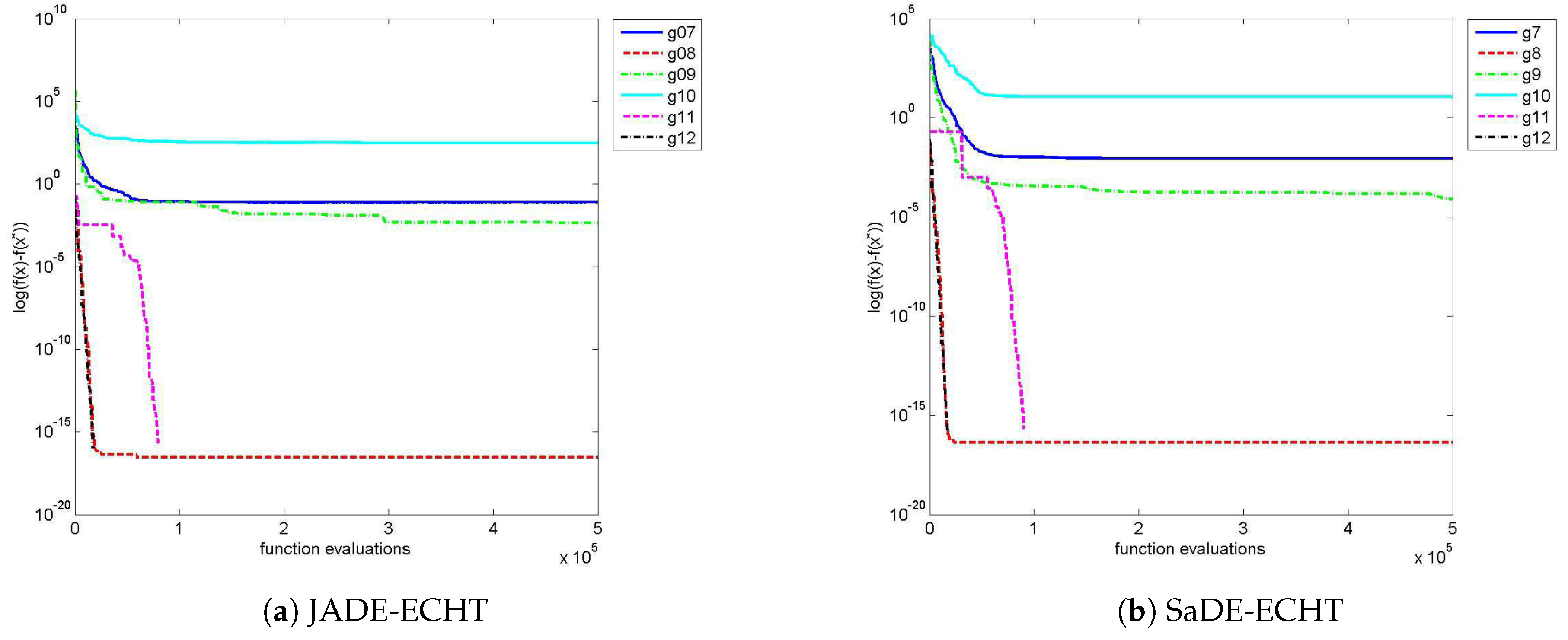
Table 4 presents the experimental statistics achieved by JADE-ECHT and SaDE-ECHT for problems g07–g12. The results of this table show that both algorithms obtained comparable statistics for problems g08, g11 and g12. This table also shows superior performance of SaDE-ECHT in terms median, mean and standard deviation values than JADE-ECHT on the problems g07, g09 and g10 except the best values on problems g07 and g10, where JADE-ECHT got better best values. The table also confirms that both algorithms have achieved $100\%$ FR on all six problems, as can be seen from the $0s$ in parenthesis after the objective function values, and columns for c and $\overline{v}$. The SR of JADE-ECHT on problems g07 and g10 is higher than SaDE-ECHT. SaDE-ECHT’s SR is better than JADE-ECHT on problem g09, while both algorithms obtained the same SR of $100\%$ on problems g08, g11 and g12.

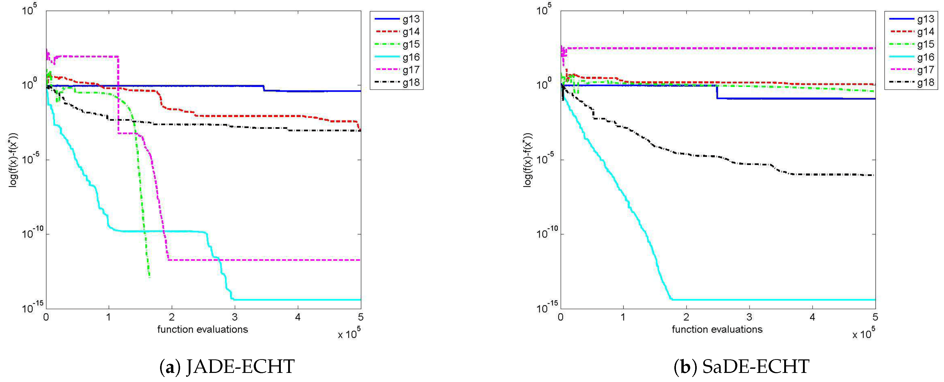
Table 5 demonstrates the experimental results achieved by JADE-ECHT and SaDE-ECHT for problems g13–g18. The results of this table show that both algorithms performed similar on problem g16. This table also shows superior performance of SaDE-ECHT in terms best, median, mean and standard deviation values than JADE-ECHT on problems g13 and g18 except the standard deviation of g13, while JADE-ECHT performed better than SaDE-ECHT on problems g14, g15 and g17 except the mean and standard deviation values of problem g14, where SaDE-ECHT got better values for the two quantities. The table also confirms that both algorithms have achieved $100\%$ FR on all six problems, as can be seen from the $0s$ in parenthesis after the objective function values, and columns for c and $\overline{v}$. The SR of JADE-ECHT on problems g14, g15, and g17 is higher than SaDE-ECHT. SaDE-ECHT’s SR is better than JADE-ECHT on problems g13 and g18, while both algorithms obtained the same SR of $100\%$ on problem g16.

Table 6 presents the experimental results achieved by JADE-ECHT and SaDE-ECHT for problems g19–g24. The results of this table show that both algorithms performed similar on problem g24. This table also shows superior performance of JADE-ECHT in terms best, median, mean and standard deviation values than SaDE-ECHT on problems g19, g20 g21 and g23, except the best value of problem g20 and standard deviation value of problem g23, while SaDE-ECHT performed better than JADE-ECHT on problem g22. The table also confirms that both algorithms have achieved $100\%$ FR on problems g19 and g24, as can be seen from the $0s$ in parenthesis after the objective function values, and columns for c and $\overline{v}$. Both algorithms are unsuccessful in solving problems g20 and g20. The FR of JADE-ECHT on problem g21 is lower than SaDE-ECHT, while the situation is vice versa in case of SR. The FR and SR of JADE-ECHT on problem g23 is higher than SaDE-ECHT.

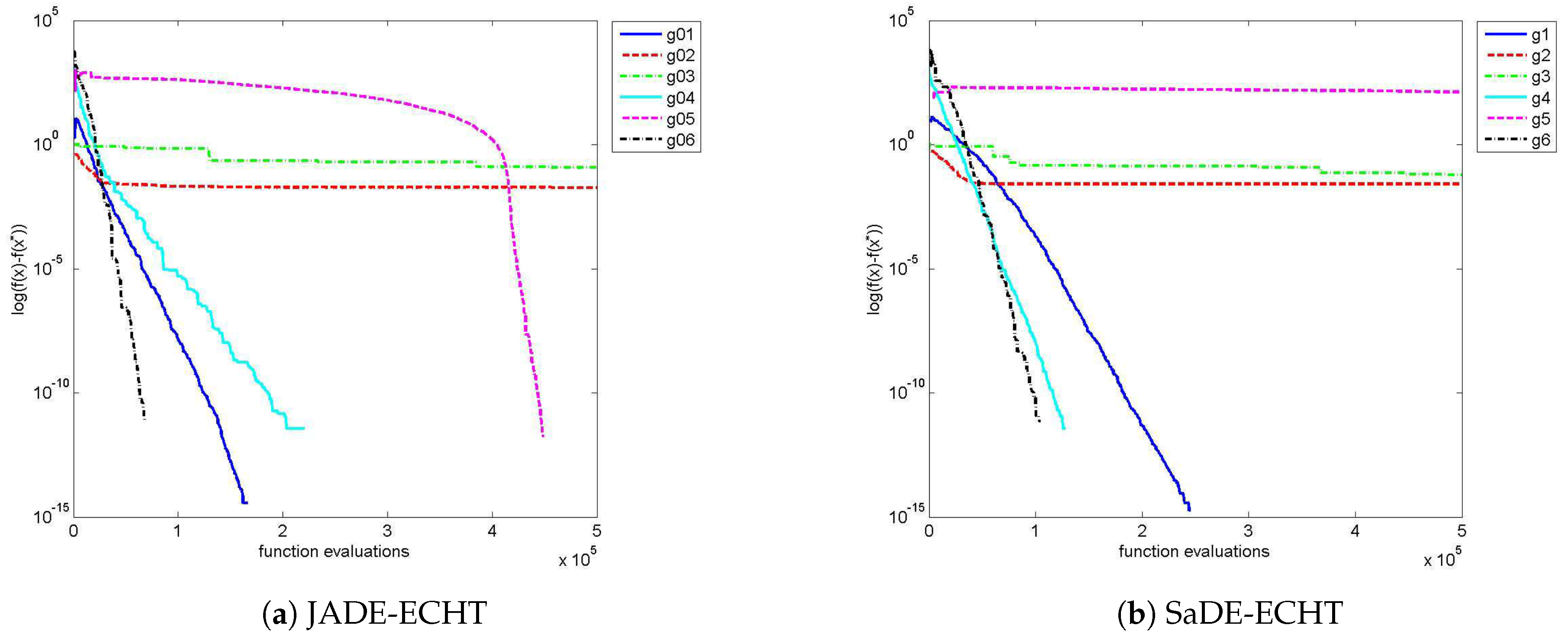
Figure 3 compares the convergence graphs of JADE-ECHT and SaDE-ECHT for problems g01–g06. This figure shows that JADE-ECHT converges faster than SaDE-ECHT on problems g01, g05 and g06, as less number of $FEs$ have been used by it. In case of problem g04, the convergence of SaDE-ECHT is speedy than JADE-ECHT, while in case of problems g02, g03 both algorithms converge at the same rate.

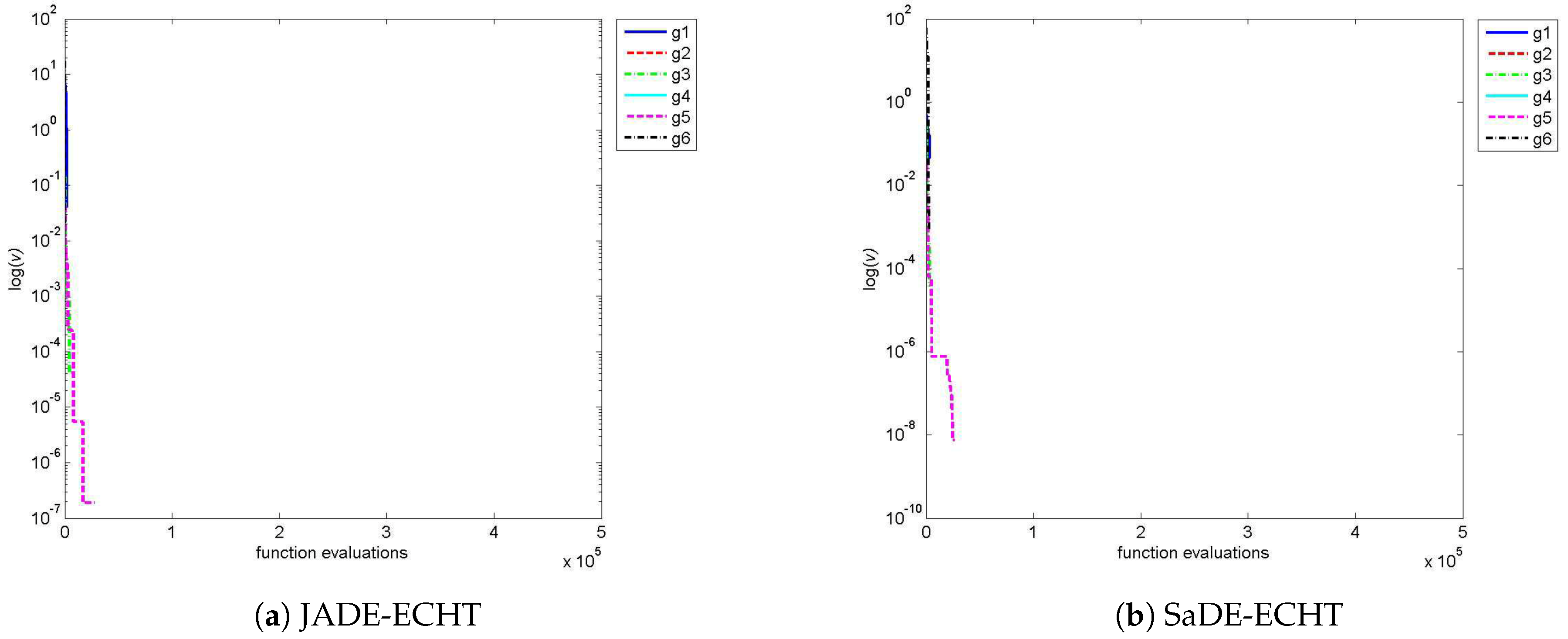
Figure 4 compares the constraints’ violations vs $FES$ graphs of JADE-ECHT and SaDE-ECHT for problems g01–g06. This figure shows that both algorithms converge quickly to the feasible region and the optimal solution (s) thus has zero constraints’ violations.

Figure 5 compares the convergence graphs of JADE-ECHT and SaDE-ECHT for problems g07–g12. This figure shows that both JADE-ECHT and SaDE-ECHT converge at the same rate for all six problems except g11, where JADE-ECHT converges faster than SaDE-ECHT.

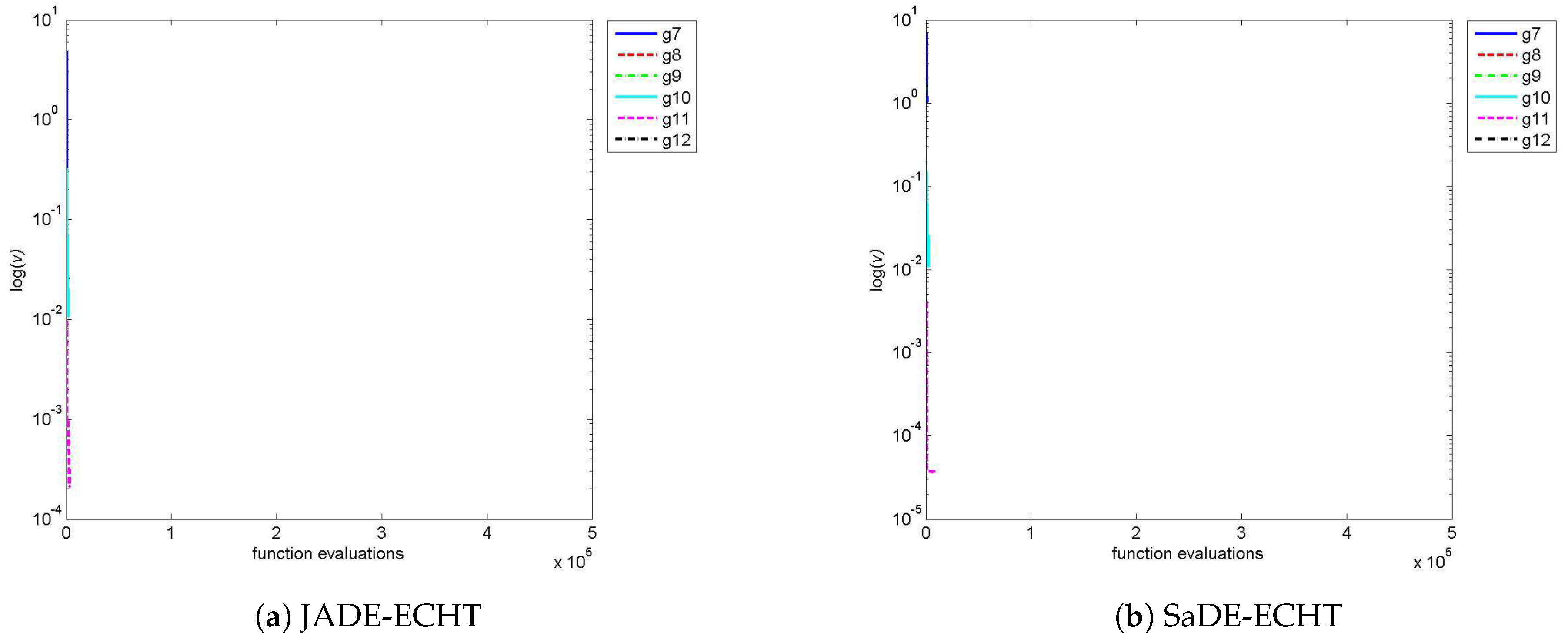
Figure 6 compares the constraints’ violations vs $FES$ graphs of JADE-ECHT and SaDE-ECHT for problems g07–g12. This figure too shows that both algorithms converge quickly to the feasible region and optimal solution(s) thus has zero constraints’ violations.

Figure 7 compares the convergence graphs of JADE-ECHT and SaDE-ECHT for problems g13–g18. This figure shows that both JADE-ECHT and SaDE-ECHT converge at the same rate for all six problems except g15, where JADE-ECHT converges faster than SaDE-ECHT.

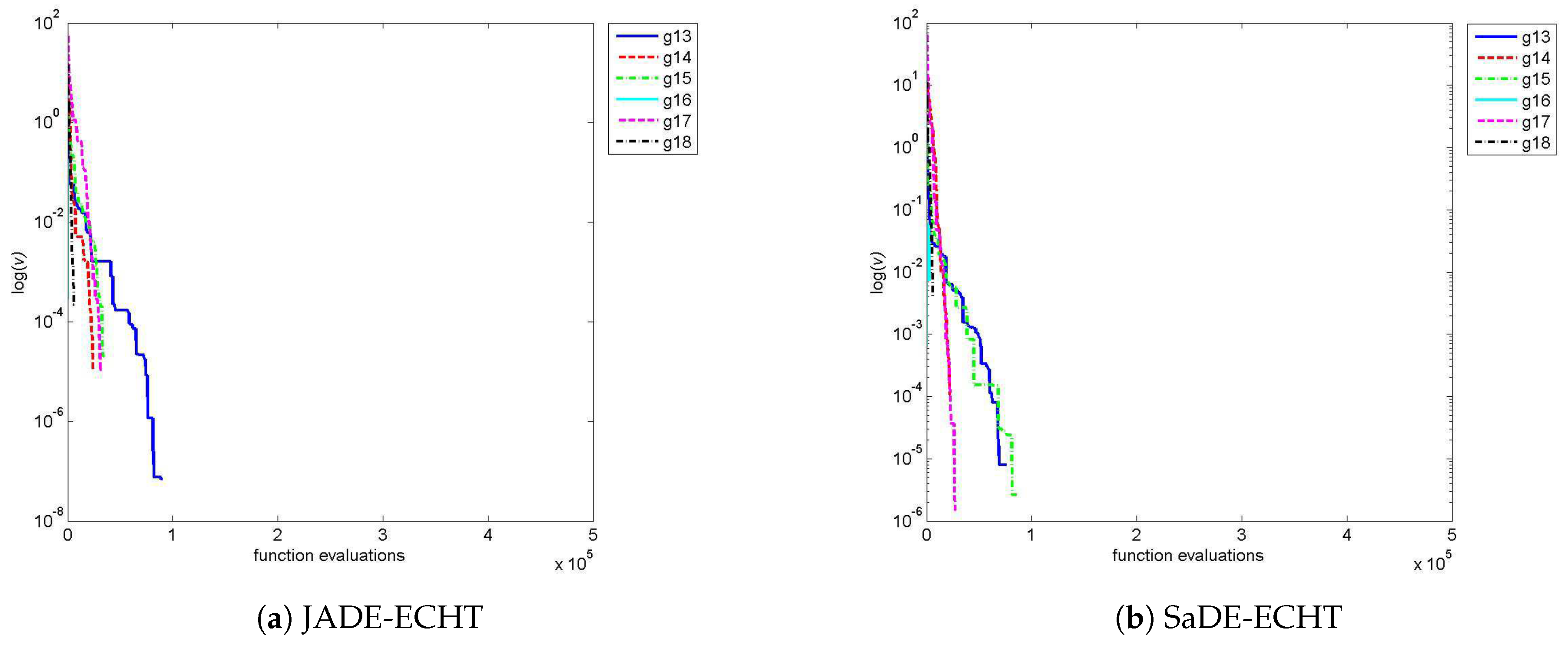
Figure 8 compares the constraints’ violations vs $FES$ graphs of JADE-ECHT and SaDE-ECHT for problems g13–g18. This figure shows that both algorithms explore the infeasible region for about 1000 iterations and then converge to the feasible region. As a result, optimal solution(s) thus obtained has zero constraints’ violations.

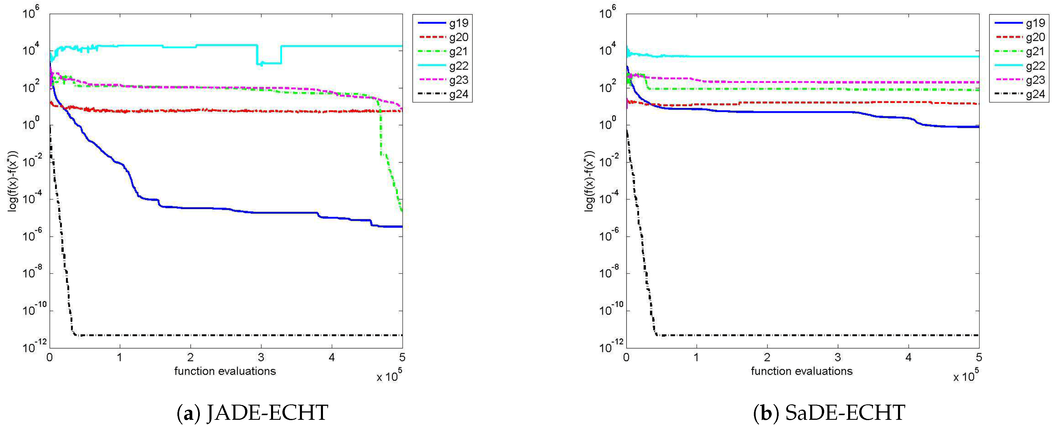
Figure 9 compares the convergence graphs of JADE-ECHT and SaDE-ECHT for problems g19–g24. This figure shows that both JADE-ECHT and SaDE-ECHT converge almost at the same rate for all six problems and utilize the maximum function evaluations.

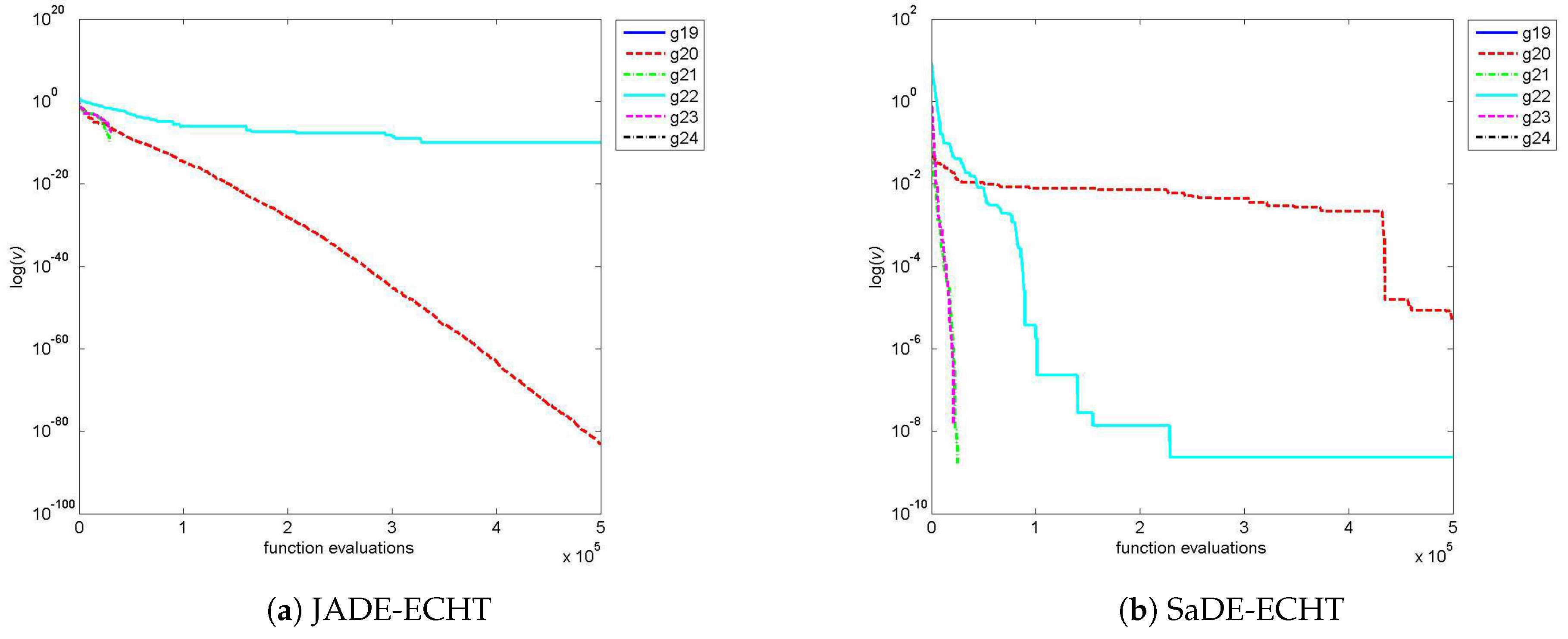
Figure 10 compares the constraints’ violations vs $FES$ graphs of JADE-ECHT and SaDE-ECHT for problems g19–g24. This figure clearly shows that both algorithms failed to obtain any feasible solution in case of problems g20 and g22, although maximum function evaluations have been used.

Figure 3, Figure 5, Figure 7 and Figure 9 show the comparison of the convergence graphs vs $FES$ of both algorithms for all problems g01-g24, whereas Figure 4, Figure 6, Figure 8 and Figure 10 demonstrate their comparison graphs of the constraints’ violations vs $FEs$.

Overall, it can be concluded from the tabulated results and figures that both algorithms have achieved feasible solution (s) and near optimal solution (s) on 22 problems out of 24 except problems g20 and g22. The tables show that the FR of JADE-ECHT on 20 problems out of 24 is $100\%$ and that of SaDE-ECHT on 22 problems out of 24 is $100\%$. The SR of JADE-ECHT on most of the problems is better than SaDE-ECHT. On two problems g20 and g22, the FR and SR of both algorithms are 0%. The dimension of these two problems is higher than other 22 problems. Also, these two problems had a large number of equality constraints. It can be noted from our experiments and some other literature review that equality constraints were hard to handle.

Table 7. Comparison of JADE-ECHT and SaDE-ECHT in terms of feasibility rate (FR) and success rate (SR) with algorithms of CEC 2006.

Algorithms	FR	SR
DE	95.65%	78.09%
DMS-PSO	100%	90.61%
$ϵ$ DE	100%	95.65%
GDE	92.00%	77.39%
jDE-2	95.65%	80.00%
MDE	95.65%	87.65%
MPDE	94.96%	87.65%
PCX	95.65%	94.09%
PESO+	95.48%	67.83%
SaDE	100%	87.13%
JADE-ECHT	95.30%	57.04%
SaDE-ECHT	95.65%	46.43%

compares the FR and SR of JADE-ECHT and SaDE-ECHT with other competing algorithms of CEC’2006. It can be seen from the said table that both JADE-ECHT and SaDE-ECHT achieved better FR, and can be placed at positions second and fourth, respectively. However, they failed to achieve better SR than the competing algorithms. A reason of failure could be the use of four different CHTs, where the resources ($FEs$) are distributed based on the success of each individual CHT, while the competing algorithms used just one CHT. The same can also be observed from

Table 8. Comparison of median values of JADE-ECHT, SaDE-ECHT and CEC’2006 algorithms achieved after 500,000 FEs. The bold numbers indicate the better results.

Prob	DE	DMS-PSO	$\mathit{ϵ}$ DE	GDE	jDE-2	MDE	MPDE	PCX	PESO+	SaDE	JADE-ECHT	SaDE-ECHT
g01	0(0)	0(0)	0(0)	0(0)	0(0)	0(0)	0(0)	0(0)	0(0)	0(0)	0(0)	0(0)
g02	5.1700 $\times {10}^{-8}$ (0)	0(0)	3.0933 $\times {10}^{-8}$(0)	2.3251 $\times {10}^{-7}$(0)	3.3051 $\times {10}^{-9}$(0)	0.017460(0)	3.5608 $\times {10}^{-6}$	0(0)	1.4314 $\times {10}^{-6}$(0)	3.0800 $\times {10}^{-9}$(0)	0.0004(0)	0.0110(0)
g03	6.7110 $\times {10}^{-1}$(0)	0(0)	−4.4409 $\times {10}^{-16}$(0)	9.3634 $\times {10}^{-1}$(0)	0.3481(0)	0(0)	−2.8866 $\times {10}^{-15}$	0(0)	1.5890 $\times {10}^{-7}$ (0)	1.7770 $\times {10}^{-8}$(0)	0.1015(0)	0.0122(0)
g04	7.6398 $\times {10}^{-11}$(0)	0(0)	0(0)	8.0036 $\times {10}^{-11}$(0)	0(0)	0(0)	3.6380 $\times {10}^{-12}$	0(0)	1.0000 $\times {10}^{-10}$(0)	2.1667 $\times {10}^{-7}$(0)	0(0)	0(0)
g05	−9.0949 $\times {10}^{-13}$(0)	0(0)	0(0)	0(0)	0(0)	0(0)	0(0)	0(0)	0(0)	0(0)	0(0)	91.4773(0)
g06	4.5475 $\times {10}^{-11}$	0(0)	1.1823 $\times {10}^{-11}$(0)	6.1846 $\times {10}^{-11}$(0)	1.1823 $\times {10}^{-11}$(0)	0(0)	1.0914 $\times {10}^{-11}$	0(0)	1.0000 $\times {10}^{-10}$(0)	4.5475 $\times {10}^{-11}$(0)	0(0)	0(0)
g07	7.9783 $\times {10}^{-11}$(0)	0(0)	−1.8474 $\times {10}^{-13}$(0)	3.6402 $\times {10}^{-10}$(0)	−1.8829 $\times {10}^{-13}$(0)	0(0)	−1.8474 $\times {10}^{-13}$	0(0)	9.4367 $\times {10}^{-6}$(0)	1.4608 $\times {10}^{-7}$(0)	0.0879(0)	0.0114(0)
g08	8.1964 $\times {10}^{-11}$(0)	0(0)	4.1633 $\times {10}^{-17}$(0)	8.1964 $\times {10}^{-11}$(0)	4.1633 $\times {10}^{-17}$(0)	0(0)	4.1633 $\times {10}^{-17}$	0(0)	1.0000 $\times {10}^{-10}$(0)	8.1964 $\times {10}^{-11}$(0)	0(0)	0(0)
g09	−9.8112 $\times {10}^{-11}$(0)	0(0)	0(0)	−9.7884 $\times {10}^{-11}$(0)	2.2737 $\times {10}^{-13}$(0)	0(0)	1.1369 $\times {10}^{-13}$	0(0)	1.0000 $\times {10}^{-10}$(0)	3.7440 $\times {10}^{-7}$(0)	0.0039(0)	0(0)
g10	6.2755 $\times {10}^{-11}$(0)	1.0124 $\times {10}^{-8}$(0)	−9.0949 $\times {10}^{-13}$(0)	6.9122 $\times {10}^{-11}$(0)	−9.0949 $\times {10}^{-13}$(0)	0(0)	−9.0949 $\times {10}^{-13}$	0(0)	1.3432 $\times {10}^{-3}$(0)	1.8120 $\times {10}^{-6}$(0)	133.9677(0)	0.1709(0)
g11	0(0)	0(0)	0(0)	0(0)	0(0)	0(0)	0(0)	0(0)	0(0)	0(0)	0(0)	0(0)
g12	0(0)	0(0)	0(0)	0(0)	0(0)	0(0)	0(0)	0(0)	0(0)	0(0)	0(0)	0(0)
g13	3.8486 $\times {10}^{-1}$(0)	0(0)	9.7145 $\times {10}^{-17}$(0)	3.8486 $\times {10}^{-1}$(0)	0.6800(0)	0(0)	3.8486 $\times {10}^{-1}$	0(0)	1.1200 $\times {10}^{-8}$(0)	4.1898 $\times {10}^{-11}$(0)	0.9118(0)	0.3870(0)
g14	8.5123 $\times {10}^{-12}$(0)	0(0)	2.1316 $\times {10}^{-14}$(0)	6.3148 $\times {10}^{-8}$(0)	2.1316 $\times {10}^{-14}$(0)	0(0)	−3.9961 $\times {10}^{-4}$	0(0)	3.2912 $\times {10}^{-3}$(0)	1.4793 $\times {10}^{-5}$(0)	0.0174(0)	1.6397(0)
g15	6.0822 $\times {10}^{-11}$(0)	0(0)	0(0)	6.0936 $\times {10}^{-11}$(0)	0(0)	0(0)	0(0)	0(0)	1.0000 $\times {10}^{-10}$(0)	6.0822 $\times {10}^{-11}$(0)	0(0)	0.0009(0)
g16	6.5214 $\times {10}^{-11}$(0)	0(0)	4.4409 $\times {10}^{-15}$(0)	6.5216 $\times {10}^{-11}$(0)	5.1070 $\times {10}^{-15}$(0)	0(0)	5.3291 $\times {10}^{-15}$	0(0)	1.0000 $\times {10}^{-10}$(0)	6.5214 $\times {10}^{-11}$(0)	0(0)	0(0)
g17	7.4058 $\times {10}^1$(0)	7.4058 $\times {10}^1$(0)	1.8190 $\times {10}^{-12}$(0)	7.4052 $\times {10}^1$(0)	10.4896(0)	0(0)	7.4058 $\times {10}^1$	0(0)	13.9638(0)	7.4058 $\times {10}^1$(0)	0(0)	91.2351(0)
g18	1.5561 $\times {10}^{-11}$(0)	0(0)	3.3307 $\times {10}^{-16}$(0)	4.6362 $\times {10}^{-11}$(0)	4.4408 $\times {10}^{-16}$(0)	0(0)	4.4409 $\times {10}^{-16}$	0(0)	4.0000 $\times {10}^{-10}$(0)	1.5561 $\times {10}^{-11}$(0)	0.0001(0)	0(0)
g19	4.6370 $\times {10}^{-11}$(0)	0(0)	5.2162 $\times {10}^{-8}$(0)	5.2669 $\times {10}^{-9}$(0)	4.2632 $\times {10}^{-14}$(0)	0.387033(0)	3.5527 $\times {10}^{-14}$	0(0)	2.6302 $\times {10}^{-2}$(0)	1.3868 $\times {10}^{-10}$(0)	1.4028(0)	1.7022(0)
g20	−2.4674 $\times {10}^{-2}$(8)	−7.3330 $\times {10}^{-2}$(17)	−2.4674 $\times {10}^{-2}$(8)	1.3503 $\times {10}^1$(20)	0.1082(2)	0.103314(20)	1.0151 $\times {10}^1$	0.0675(12)	3.2600 $\times {10}^{-2}$(8)	2.3757 $\times {10}^{-1}$(20)	6.2057(8)	14.8045(9)
g21	−2.8371 $\times {10}^{-10}$(0)	3.5911 $\times {10}^{-6}$(0)	−2.8422 $\times {10}^{-14}$(0)	6.5523 $\times {10}^{-8}$(0)	−2.8421 $\times {10}^{-14}$(0)	0(0)	1.4211 $\times {10}^{-13}$	0(0)	81.3460(0)	2.5785 $\times {10}^{-8}$(0)	0.0633(0)	77.3185(0)
g22	1.0336 $\times {10}^4$(15)	1.2200 $\times {10}^2$ (0)	1.2332 $\times {10}^1$(0)	9.7885 $\times {10}^3$(19)	8033.6537(8)	9210.082460(18)	8.7919 $\times {10}^3$	9888.6409(15)	14,198.8059(19)	4.6907 $\times {10}^1$(0)	10,565.5111(3)	8834.7836(3)
g23	3.0005 $\times {10}^2$(0)	1.0267 $\times {10}^{-8}$ (0)	0(0)	1.0569 $\times {10}^1$(0)	2.2737 $\times {10}^{-13}$(0)	0(0)	0(0)	0(0)	130.5043(0)	3.9790 $\times {10}^{-13}$(0)	8.5726(0)	357.7081(0)
g24	4.6736 $\times {10}^{-12}$(0)	0(0)	5.7732 $\times {10}^{-14}$(0)	4.7269 $\times {10}^{-12}$(0)	5.5067 $\times {10}^{-14}$(0)	0(0)	7.1054 $\times {10}^{-14}$	0(0)	0(0)	4.6372 $\times {10}^{-12}$(0)	0(0)	0(0)

and

Table 9. Comparison of standard deviation values of JADE-ECHT, SaDE-ECHT and CEC’2006 algorithms achieved after 500,000 FEs. The bold numbers indicate the better results.

Prob	DE	DMS-PSO	$\mathit{ϵ}$ DE	GDE	jDE-2	MDE	MPDE	PCX	PESO+	SaDE	JADE-ECHT	SaDE-ECHT
g01	6.4146 $\times {10}^{-15}$	0	0	0	0	0	0	0	0	0	0.4000	0
g02	1.0015 $\times {10}^{-18}$	4.6953 $\times {10}^{-3}$	1.7523 $\times {10}^{-8}$	7.5112 $\times {10}^{-3}$	3.0488 $\times {10}^{-3}$	0	2.7802 $\times {10}^{-3}$	0	7.1385 $\times {10}^{-3}$	4.9786 $\times {10}^{-3}$	0.0091	0.0254
g03	5.2098 $\times {10}^{-14}$	0	2.9582 $\times {10}^{-31}$	1.9833 $\times {10}^{-1}$	1.0140 $\times {10}^{-1}$	0	8.3681 $\times {10}^{-2}$	0	1.5396 $\times {10}^{-6}$	3.4743 $\times {10}^{-5}$	0.1036	0.0343
g04	3.9644 $\times {10}^{-13}$	0	0	0	0	0	0	0	0	1.8550 $\times {10}^{-12}$	0	0
g05	0	0	0	1.6854 $\times {10}^2$	2.4193	0	3.6380 $\times {10}^{-13}$	0	0	1.8190 $\times {10}^{-13}$	0	101.2496
g06	0	0	0	0	0	0	0	0	0	0	0	0
g07	6.4146 $\times {10}^{-15}$	0	2.1831 $\times {10}^{-15}$	3.8948 $\times {10}^{-7}$	1.7405 $\times {10}^{-15}$	0	3.0215 $\times {10}^{-15}$	0	2.2678 $\times {10}^{-5}$	1.4993 $\times {10}^{-5}$	0.0726	0.0850
g08	1.0015 $\times {10}^{-18}$	0	1.2326 $\times {10}^{-32}$	0	1.2580 $\times {10}^{-32}$	0	0	0	0	3.8426 $\times {10}^{-18}$	0	0
g09	5.2098 $\times {10}^{-14}$	0	0	4.9555 $\times {10}^{-14}$	4.2538 $\times {10}^{-14}$	0	0	0	0	7.9851 $\times {10}^{-14}$	0.0192	0.0002
g10	3.9644 $\times {10}^{-13}$	8.8141 $\times {10}^{-9}$	4.2426 $\times {10}^{-13}$	0	9.1279 $\times {10}^{-8}$	0	3.0165 $\times {10}^{-13}$	0	5.8279 $\times {10}^{-2}$	1.5244 $\times {10}^{-6}$	105.4501	3.0352
g11	0	0	0	0	4.5540 $\times {10}^{-4}$	0	7.0638 $\times {10}^{-5}$	0	0	0	0	0
g12	0	0	0	0	0	0	0	0	0	0	0	0
g13	0	1.8204 $\times {10}^{-6}$	0	3.8650 $\times {10}^{-1}$	2.2376 $\times {10}^{-1}$	0	2.8719 $\times {10}^{-1}$	0	6.3801 $\times {10}^{-6}$	2.7832 $\times {10}^{-7}$	0.1750	0.2828
g14	3.4809 $\times {10}^{-15}$	0	1.3924 $\times {10}^{-15}$	3.8556 $\times {10}^{-3}$	3.4809 $\times {10}^{-15}$	0	7.9441 $\times {10}^{-15}$	0	2.8553 $\times {10}^{-2}$	6.4986 $\times {10}^{-5}$	2.2940	0.6956
g15	0	0	0	9.6094 $\times {10}^{-1}$	2.2020 $\times {10}^{-2}$	0	4.3027 $\times {10}^{-6}$	0	0	0	0	0.6971
g16	2.2092 $\times {10}^{-16}$	0	1.5777 $\times {10}^{-30}$	1.7764 $\times {10}^{-16}$	0	0	0	0	0	0	0	0
g17	3.0234 $\times {10}^1$	0	1.2117 $\times {10}^{-27}$	8.2114 $\times {10}^1$	3.8319 $\times {10}^1$	0	3.4111 $\times {10}^1$	0	42.286	1.6168 $\times {10}^1$	24.5623	50.4589
g18	4.8817 $\times {10}^{-17}$	0	2.1756 $\times {10}^{-17}$	6.4619 $\times {10}^{-1}$	3.6822 $\times {10}^{-17}$	0	4.1541 $\times {10}^{-17}$	0	3.8184 $\times {10}^{-2}$	5.2898 $\times {10}^{-2}$	0.0041	0
g19	1.2568 $\times {10}^{-5}$	0	1.2568 $\times {10}^{-5}$	4.5735 $\times {10}^{-5}$	1.0531 $\times {10}^{-13}$	0.847517	3.5527 $\times {10}^{-14}$	0	1.6158 $\times {10}^{-1}$	7.2976 $\times {10}^{-10}$	1.0136	1.9699
g20	4.2362 $\times {10}^{-2}$	6.9516 $\times {10}^{-3}$	4.2362 $\times {10}^{-2}$	1.9580 $\times {10}^0$	1.1510 $\times {10}^{-2}$	0.021688	2.8984 $\times {10}^0$	0.0219	4.9951 $\times {10}^{-3}$	1.0638 $\times {10}^{-1}$	3.5087	4.8304
g21	6.5489 $\times {10}^1$	2.0784 $\times {10}^{-6}$	3.3417 $\times {10}^{-14}$	8.6788 $\times {10}^1$	3.6266 $\times {10}^1$	0	6.2358 $\times {10}^1$	0	67.019	1.5058 $\times {10}^{-3}$	63.9006	25.3368
g22	5.7875 $\times {10}^3$	2.7703 $\times {10}^1$	1.5690 $\times {10}^1$	5.9865 $\times {10}^3$	5.1748 $\times {10}^3$	4808.800969	4.8022 $\times {10}^3$	4421.5326	4963.7	3.0415 $\times {10}^1$	6162.3243	4998.2886
g23	8.8097 $\times {10}^{-6}$	4.5997 $\times {10}^{-4}$	1.1139 $\times {10}^{-14}$	1.9119 $\times {10}^2$	5.9983 $\times {10}^1$	0	5.1159 $\times {10}^{-14}$	0	87.634	3.4116 $\times {10}^{-4}$	198.2664	87.4764
g24	8.8525 $\times {10}^{-20}$	0	2.5244 $\times {10}^{-29}$	0	1.9323 $\times {10}^{-29}$	0	0	0	0	0	0	0

, where the median and standard deviation values obtained after $5\times {10}^5$ $FEs$ of JADE-ECHT and SaDE-ECHT are compared with other competing algorithms (the values of the two quantities for the competing algorithms are taken from each source paper). Another reason of low SR could be observed from the figures showing constraints’ violations vs $FES$ graphs. It can be noticed from these graphs that both algorithms converge quickly to the feasible region. As a result, they less explore the infeasible region and consequently suffer from stagnation and premature convergence.

5. Conclusions and Future Work

This paper employed ECHT in the frameworks of two self-adaptive variants of DE, JADE and SaDE. Thus, constrained versions of the two algorithms, denoted by JADE-ECHT and SaDE-ECHT were developed. The proposed algorithms JADE-ECHT and SaDE-ECHT were tested and compared on CEC’06 benchmark test suit. The experimental results show that the SR of JADE-ECHT on most of the tested problems is better than SaDE-ECHT, while SaDE-ECHT surpasses JADE-ECHT in terms of FR. Both algorithms, like other algorithms in the literature, failed to solve problems g20 and g22 due to the hard nature of these problems. In the future, we intend to design ECHT of some other CHTs, embed it then in DE and swarm based algorithms to develop constrained evolutionary algorithms and finally test these newly developed algorithms on some real-world and engineering optimization problems. In addition to that we are going to use [34] for multipath routing protocols and for video streaming systems [35] in order to get the advantages of these plus the benefits of the proposed work would be very beneficent and demanded.