Efficient and Effective Directed Minimum Spanning Tree Queries

Abstract

Computing directed Minimum Spanning Tree ($DMST$) is a fundamental problem in graph theory. It is applied in a wide spectrum of fields from computer network and communication protocol design to revenue maximization in social networks and syntactic parsing in Natural Language Processing. State-of-the-art solutions are online algorithms that compute $DMST$ for a given graph and a root. For multi-query requirements, the online algorithm is inefficient. To overcome the drawbacks, in this paper, we propose an indexed approach that reuses the computation result to facilitate single and batch queries. We store all the potential edges of $DMST$ in a hierarchical tree in $O\left(n\right)$ space complexity. Furthermore, we answer the $DMST$ query of any root in $O\left(n\right)$ time complexity. Experimental results demonstrate that our approach can achieve a speedup of 2–3 orders of magnitude in query processing compared to the state-of-the-art while consuming O(n) index size.

1. Introduction

Finding a $DirectedMinimumSpanningTree$$\left(DMST\right)$, which is also known as the Minimum Cost Arborescence problem, in a given directed graph is one of the fundamental problems in graph theory. For a directed graph G, given root r, the query aims to find a $DMST$ rooted at r that connects all the vertices.

$DMST$ can be applied to many fields. In communication, it is implemented for minimum cost connectivity [1,2] and control [3]. In the database, it is utilized for reachability queries [4,5]. In natural language processing, it is a classic dependency parsing algorithm [6,7,8,9]. In visualization, it captures information [10,11] and facilitates genetic analysis [12,13,14]. In social networks, it evaluates influence [15] and information flows [16,17].

Chu-Liu and Edmonds [1,18] proposed an algorithm that answers the query in $O\left(mn\right)$ time complexity, where n is the number of vertices in the graph and m is the number of edges. Their algorithm is a two-phase algorithm that involves contraction and expansion. Tarjan [19] then proposed a faster implementation in $O(mlogn)$ time for sparse graphs and $O\left(n^2\right)$ for dense ones. Gabow et al. [20] improved their algorithms by implementing a Fibonacci heap. By utilizing the $O\left(1\right)$$uniteoperation$ feature and a depth-first strategy, their algorithm is able to return a $DMST$ in $O(m+nlogn)$ time.

Motivation. All of the above algorithms are online algorithms. For a series of queries on the same graph with different roots, they have to repeat the computing procedure for every single root in the graph. However, we find that for different roots, the corresponding $DMST$s always contain edges of minimum weight related to vertices. We build an index that chooses and stores the edge of the minimum weight for each vertex. Therefore, the computing time for the $DMST$ query can be saved by only referring to the edges in the index instead of searching the original graph.

Our Idea. In this paper, we propose an index-based approach for the $DMST$ problem rooted at any vertex on the given directed graph. We first keep track of all potential edges of any $DMST$ in the given graph and store them in a hierarchical tree. Then we find the $DMST$ of the given root by choosing edges in the tree index. The index computing time is $O\left(mn\right)$, which is the same time cost as [1,18]. The query time for any given root is $O\left(n\right)$. Furthermore, the space complexity is $O\left(n\right)$.

The contribution of this paper can be summarized as follows:

• We are the first to propose an efficient indexed approach for the $DMST$ problem. We can answer a single query at any root in the graph in $O\left(n\right)$ time. Furthermore, we can process batch queries even faster.
• We prove the correctness of our algorithms. Furthermore, we prove that both single and batch algorithms take worst-case $O\left(n\right)$ space and time complexity.
• We conduct our algorithms on different directed graph datasets to show the efficiency and effectiveness of our algorithms.

2. Related Work

$DMST$ can be applied to a wide spectrum of fields. Since the directed maximum spanning tree can be found with the same algorithm by trivially negating the edge cost, we show its applications as follows:

Communication. $DMST$ of a communication network means the lowest cost way to propagate a message to all other nodes in G [1]. To address the connectivity issue in heterogeneous wireless networks, N. Li et al. [2] proposed a localized $DMST$ algorithm that preserves the network connectivity. The problem of containment control with the minimum number of leaders can be converted into a directed minimum spanning tree [3].

Database Management. To efficiently answer reachability queries, Jin et al. [5] created a path-graph and formed a path-tree cover for the directed graph by extracting a maximum directed spanning tree. Further, they introduced a novel tree-based index framework that utilizes the directed maximal weighted spanning tree algorithm and sampling techniques to maximally compress the generalized transitive closure for the labeled graphs [4].

Natural Language Processing. To generalize the projective parsing method to non-projective languages, McDonald et al. [7] formalized weighted dependency parsing as searching for maximum spanning trees in directed graphs. Furthermore, Smith et al. [8] found a directed maximum spanning tree for maximum $aposteriori$ decoding. Moreover, in [9], the authors couched statistical sentence generation as a spanning tree problem and found the $DMST$ of a dependency tree with maximal probability. Yang et al. [6] used $DMST$ as a tool in the evaluation of the induced structure of their proposed structured summarization model.

Visualization. For the purpose of capturing 3D surface measurements with structured light, Brink et al. [10] considered all connections and adjacencies among stripe pixels in the form of a weighted directed graph and indexed the patterns by a maximum spanning tree. Mahshad et al. [11] applied $DMST$ in handwritten math formula recognition. $DMST$ is implemented in GrapeTree [12] to visualize genetic relations and helps genetic analysis in lineage tracing [13] and cancer evolution [14].

Social Networks. For social network hosts to achieve maximum revenue in viral marketing, Zehnder [15] extracted a $DMST$ to generate a most influential tree, which approximates a social network while preserving the most influential path. To contrast the spread of misinformation in online social networks, Marco et al. [16] modeled source identification as a maximal spanning branching problem. Furthermore, Peng et al. [17] extracted important information flows and the hierarchical structure of the networks with $DMST$.

3. Problem Statement

Let $G=(V,E)$ be a directed graph where $V\left(G\right)$ is the set of vertices and $E\left(G\right)$ is the set of arcs. Arc is a directed edge starting from u to v. We use V and A to denote $V\left(G\right)$ and $E\left(G\right)$, and $n=\left|V\right|$ and $m=\left|E\right|$ to denote the number of vertices and arcs in the directed graph. We use edge to denote arc if the context is clear. We use $e=\langle u,v\rangle$ to denote the arc, where u is the tail of the arc, denoted as $tail\left(e\right)$, and v is the head, denoted as $head\left(e\right)$. We use $in$-$edge$ to denote any arc incident on a vertex as the head and $out$-$edge$ to denote any arc direct away from a vertex as the tail. Each arc $\langle u,v\rangle$ is associated with a positive cost $\varphi \langle u,v\rangle$. For each $v\in V$, we use $in\left(v\right)$ to denote all the in-edges of v, and we use $out\left(v\right)$ to denote all the out-edges of v. A path is a sequence of vertices $p=\{v_1,v_2,\dots ,v_e\}$, where $\langle v_i,v_{i+1}\rangle \in E$ and $\forall v_i,v_j\in p$, $v_i\ne v_j$. The summary of notations is in

Table 1. The summary of notations.

Notation	Definition
$G=(V,E)$	The directed graph G, vertex set V and arc set E
n, m	number of vertices n, number of arcs m
$e=\langle u,v\rangle$	arc e, from u to v, where u is tail, v is head
$\varphi \langle u,v\rangle$	cost of arc $\langle u,v\rangle$
$head\left(e\right)$, $tail\left(e\right)$	head and tail of the arc e
$in\left(v\right)$, $out\left(v\right)$	all the in-edges whose head is v, all the out-edges whose tail is v
$\mathcal{T},{\mathcal{T}}_v$	any $DMST$ of graph G, $DMST$ rooted at v
H	hierarchical tree of G containing potential $DMST$ arcs
$c_i$, $T{N}_i$, $TN\left(v\right)$	cycle, its corresponding tree node, and tree node containing v
C	set of cycles

. If there is no path from a vertex to any other vertices in the graph, the $DMST$ rooted at the vertex will cost infinity, which is meaningless. Therefore, for simplicity, in the rest of this paper, we assume that G is strongly connected. As we can obtain the maximum directed spanning tree by simply negating each edge, we focus on answering the minimum one.

Problem Definition. Given a directed graph $G=(V,E)$ and a root vertex $r\in V$, a $DirectedSpanningTree$ is an acyclic subgraph T of G that has all the vertices of G. For each vertex $v\in T$ and $v\ne r$:

(1) There is a path starting from r to v.

(2) v has only one in-edge.

A $DirectedMinimumSpanningTree$ is such a $DirectedSpanningTree$ of the minimum total edge cost.

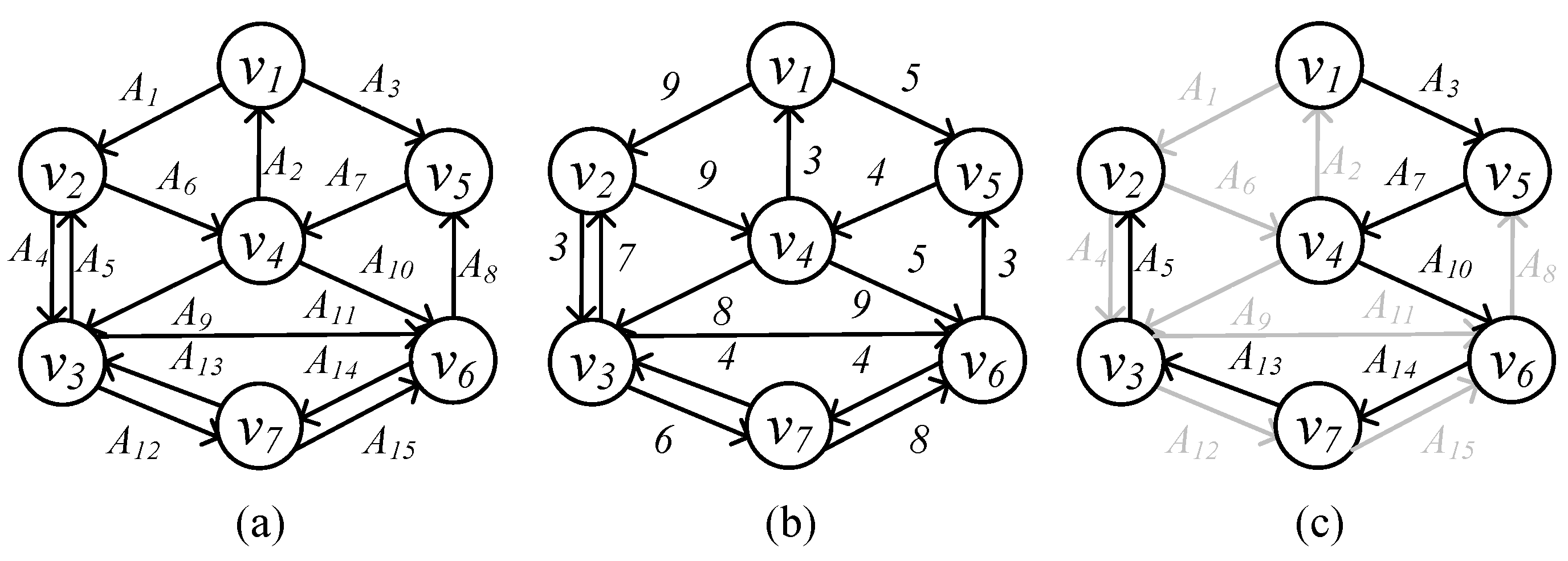
Example 1. 

In Figure 1, we show a directed graph G with 7 vertices and 15 edges. In Figure 1a, we number each edge of G. Furthermore, in Figure 1b, we show the cost of each edge. In Figure 1c, given root $v_1$, we show the directed minimum spanning tree ${\mathcal{T}}_{v_1}$ of G rooted at $v_1$. Furthermore, its total cost is 29. For each vertex $v\in {\mathcal{T}}_{v_1}$, $v\ne v_1$ there is a path from $v_1$ to v, and there is only one in-edge of each vertex in ${\mathcal{T}}_{v_1}$ except $v_1$.

4. Existing Solution

In this section, we take a review of Chu-Liu and Edmonds’ algorithm (CLE) that runs in $O\left(mn\right)$ time, and our indexed approach is based on the observations. Given a directed graph $G=(V,E)$ and a root vertex $r\in V$, CLE returns the Directed Minimum Spanning Tree $\mathcal{T}$ of r in a two-phase recursive manner. For each round of recursion, $CLE$ chooses the minimum in-edges of each vertex except r, and checks if these in-edges are a cycle. If no cycle is found, then the edges chosen this round including the root vertex r are a $DMST$. Otherwise, the cycles are contracted to a new vertex and the algorithm goes to the next round.

Contraction Phase. For each round, the algorithm first selects minimum in-edges of each vertex $v\in V\backslash r$, then finds cycles C of the selected edges. Each such cycle $c_i\in C$ found this round is contracted to a new vertex $v^{\prime }$. All vertices $v^{\prime }$ and $v\in V$ and $v\notin C$ will be added to the new vertex set $V^{\prime }$. The cost of edges $\langle u,v\rangle$, $v\notin C$ remains the same. The cost of edges $\langle u,v\rangle$, $u\notin C$, $v\in C$ will be updated as $\varphi \langle u,v\rangle -min\left\{\varphi \right(in\left(v\right)\left)\right\}$. All edges will be added to a new edge set $E^{\prime }$, and now we have $G^{\prime }=(V^{\prime },E^{\prime })$. The algorithm finds and contracts cycles in a recursive manner until there are no cycles found, as the in-edge of root r is not considered. Then the algorithm starts to expand T of this round.

Expansion Phase. For the current round, the algorithm starts from root r and breaks cycles. For each $\langle u,v\rangle \in T$, $u\notin c_i$, $v\in c_i$, $c_i\subset C$, the algorithm recovers its original cost, deletes the in-edge $\left\{\langle w,v\rangle \right|w\in c_i\}$ incident on v in cycle $c_i$ and adds it to T. Furthermore, the algorithm adds the edges in $c_i$ except $\left\{\langle w,v\rangle \right|w\in c_i\}$ to T. The algorithm returns T to the previous round until the final T is found. Here is the framework of the Algorithm 1:

Algorithm 1: CLE $(G,T,C,r)$

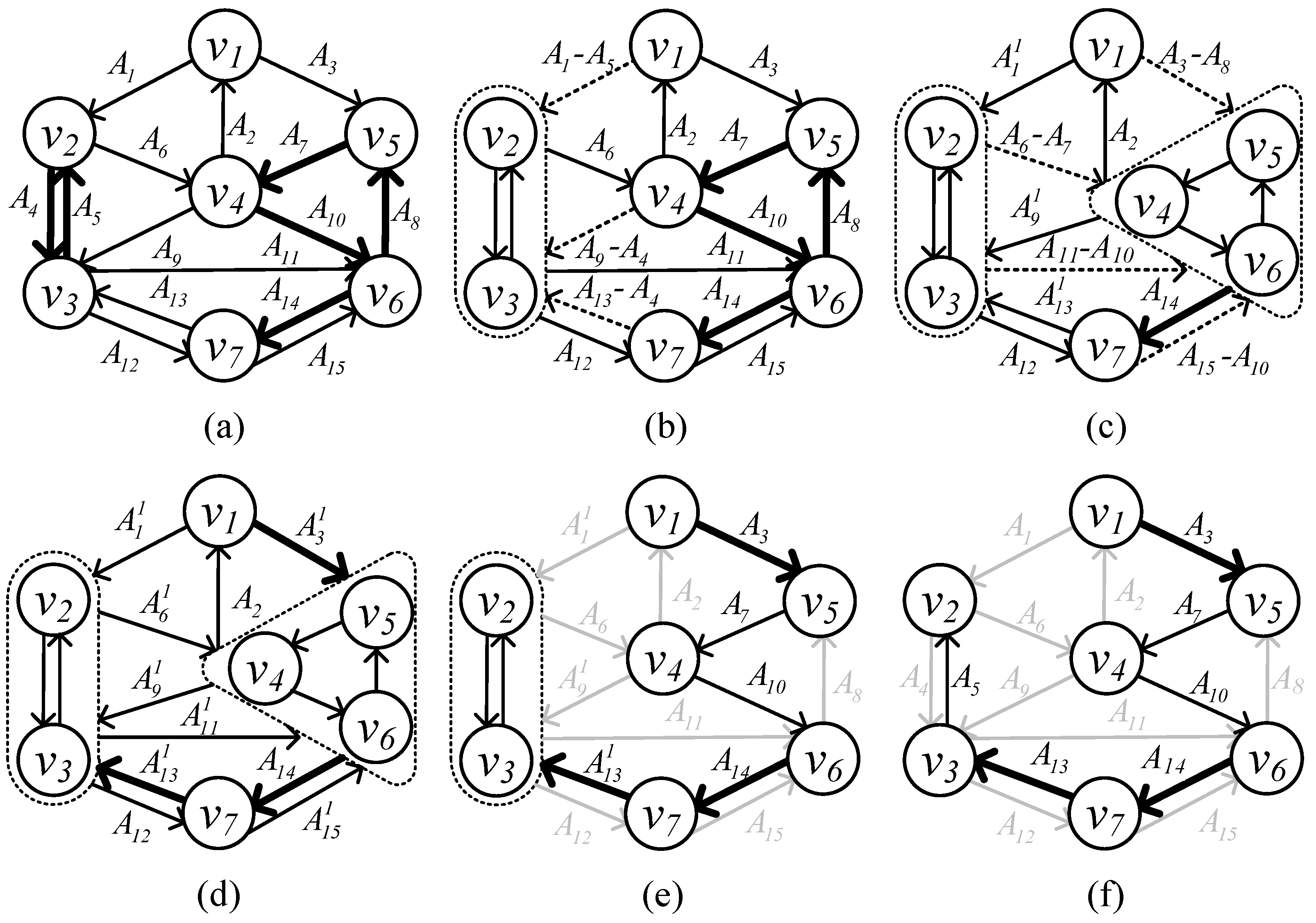
Example 2. 

We show the contraction and expansion procedure of $CLE$ algorithm at root $v_1$ in Figure 2. We denote the edge j that is updated in the ith round as $A_j^i$. In (a), for the first round, bold lines are the minimum in-edges of each vertex except the root $v_1$. In (b) and (c), $\{v_2,v_3\}$ and $\{v_4,v_5,v_6\}$ are the cycles detected in the first round and contracted to a vertex. Then, the in-edge of each cycle is updated, shown by the dashed line. By now, G is contracted to $G^{\prime }$. In (d), for the second round, in-edges of $G^{\prime }$ have no cycle. Furthermore, the contraction phase ends. The expansion phase starts from (e). In (e), for graph $G^{\prime }$, starting from out-edges of root $v_1$, $A_3^1$ is the only out-edge that starts from the root. $A_3^1$ recovers its original cost by adding back cost of $A_8$ and breaks the cycle by deleting $A_8$. In (f), $A_{13}^1$ recovers its cost by adding back cost of $A_4$ and breaks the cycle by deleting $A_4$. Furthermore, the $DMST$ rooted at $v_1$ is found.

By reviewing Chu-Liu and Edmonds’ algorithm, we have the following observations:

Observation 1. 

The cycles detected in each round have a hierarchical structure. CLE contracts and expands the cycles of the graph in a recursive manner, and generates a hierarchical structure naturally. The cycles contracted in the previous round may be a vertex of the cycles contracted in this round. Therefore, cycles of G and $G^{\prime }$ in each round can form a hierarchical structure. We can build a hierarchical tree by trivially adapting the contraction phase, detailed in Section 5.

Observation 2. 

In the expansion phase, for each cycle to break, we only need to delete one edge with both ends in the cycle. Every vertex in T has only one in-edge. The cycle $c_i\subset C$ will be contracted to a vertex $v^{\prime }$ and there will be only one minimum in-edge of $v^{\prime }$ incident on $v_k\in c_i$. Furthermore, $v_k$ has an in-edge $\langle v_{k-1},v_k\rangle$ of $c_i$. We delete $\langle v_{k-1},v_k\rangle$ so that $v_k$ has only one in-edge.

5. Our Approach

In this section, we will first analyze the drawbacks of the $CLE$ algorithm and show the hierarchical tree of the indexed edges. Then, we expand the $DMST$ with reference to the index. Finally, we elaborate on our approach to constructing the index and prove the correctness of our indexed algorithm.

5.1. Hierarchical Tree

Drawbacks of the $CLE$ algorithm. We discuss the drawbacks of the $CLE$ algorithm in terms of search space and result reuse.

Search space. For each query, $CLE$ has to find the minimum in-edge of each vertex and retrieve cycles from the original graph. Therefore, $CLE$ suffers from a large search space and spends $O\left(mn\right)$ time for the edges and cycles.

Result reuse. For a new query, $CLE$ has to restart and recompute the minimum in-edges and detect cycles. The minimum in-edges computed last time are wasted.

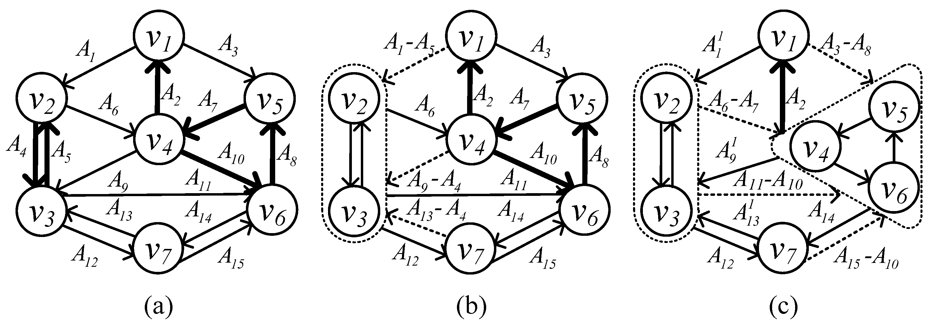
Example 3. 

For example, in Figure 3, we show the first round contraction of $CLE$ algorithm rooted at $v_7$. In (a), for the first round, we show the minimum in-edges of each vertex in bold lines except root $v_7$. In (b) and (c), $\{v_2,v_3\}$ and $\{v_4,v_5,v_6\}$ are the cycles detected in the first round and contracted to a vertex. Then the in-edge of each cycle is updated, shown by the dashed line. Now we compare with the contraction phase in Figure 2 of root $v_1$. It is obvious that edges that form the cycles $\{v_2,v_3\}$ and $\{v_4,v_5,v_6\}$ can be reused, though the $DMST$ for root $v_1$ and $v_7$ choose to delete different edges.

To solve these drawbacks, if we are able to identify the reusable edges and cycles and store them before expansion, we can choose to delete the useless edges for any given root and reduce the search space. Therefore, we propose an index that reuses the edges and cycles in the contraction phase with a trivial adaption and stores the potential edges on the hierarchical tree. By referring to the hierarchical tree, we can retrieve the $DMST$ for any given root instead of searching the entire graph. Therefore, we dramatically reduce the search space for finding the $DMST$. We make a trivial adaption by the contracting root to a vertex, and index the reusable edges and cycles on a hierarchical tree based on the following lemmas:

Lemma 1. 

For a given root r, contracting r to a vertex at any round still generates correct results.

Proof. 

For the final round h of $CLE$, as we suppose the graph is strongly connected, we add back the in-edge of the root, and the graph will be contracted to a single vertex. When the expansion starts, the in-edge of the root is removed and the lemma is true. Suppose the lemma is true for round $2=h-(h-2)$. For round 1, the root r is contracted to a new vertex $r^{\prime }$, since it is true for round 2; therefore, for root $r^{\prime }$ the expansion generates the correct result. Now by deleting the in-edge of r, we still obtain the correct result. Therefore, the lemma still holds for any round in which the root is contracted.    □

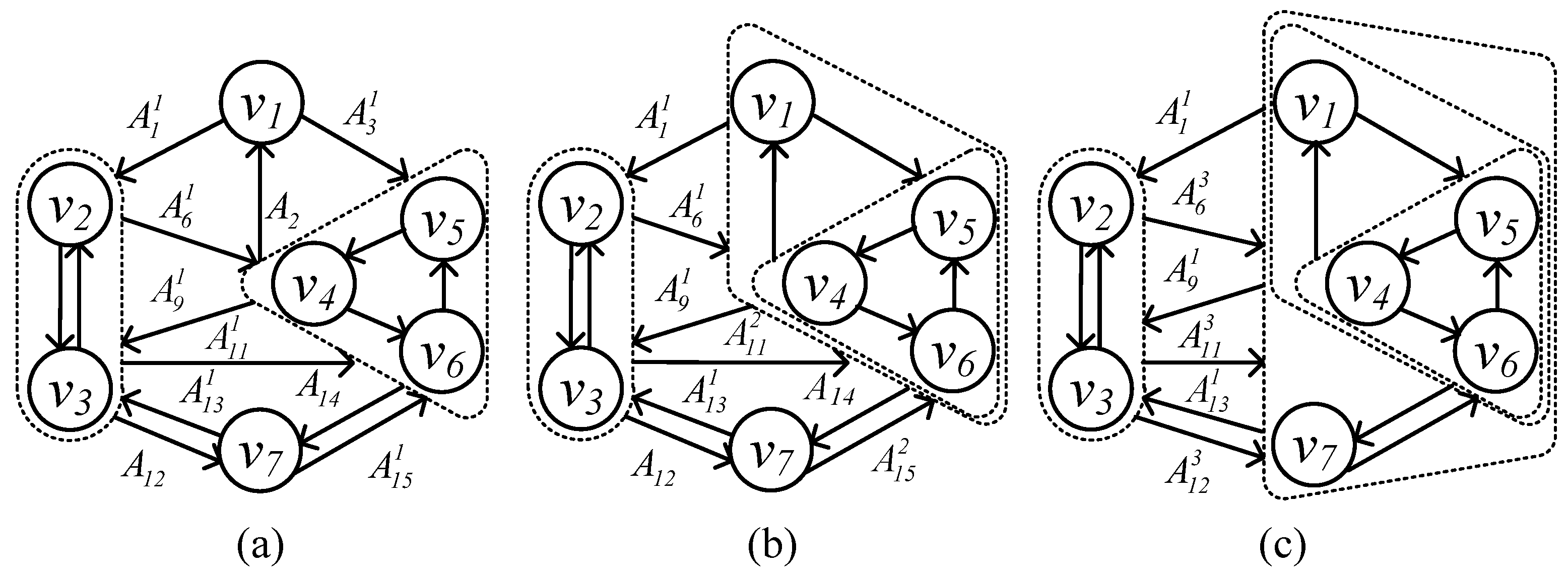
Example 4. 

We show contraction with root in Figure 4. In (a), for the first round, we find cycle $c_1=\{v_4,v_5,v_6\}$, $c_2=\{v_2,v_3\}$, and adapt in-edges of $c_1,c_2$, $A_3\to A_3^1$, $A_6\to A_6^1$, $A_{11}\to A_{11}^1$, $A_{15}\to A_{15}^1$, $A_1\to A_1^1$, $A_9\to A_9^1$, $A_{13}\to A_{13}^1$. In (b), for the second round, we find cycle $c_3=\{c_1,v_1\}$, and adapt in-edges of $c_3$, $A_6^1\to A_6^2$, $A_{11}^1\to A_{11}^2$, $A_{15}^1\to A_{15}^2$. In (c), for the third round, we find cycle $c_4=\{c_3,v_7\}$, and adapt in-edges of $c_4$, $A_6^2\to A_6^3$, $A_{11}^2\to A_{11}^3$, $A_{12}\to A_{12}^3$. Furthermore, next round we will find $c_5=\{c_4,c_1\}$. $c_5$ is not shown since it is only a single vertex.

Lemma 2. 

For any two queries with $r_1$ and $r_2$, $r_1\ne r_2$, the cycles detected in their contraction phase can be reused.

Proof. 

Since we proved in the previous lemma that contracting root at any round still generates the correct result, we follow the contraction of $r_1$ and reuse the cycles detected in its contraction phase. We prove this lemma by contradiction. Suppose that the detected cycles of $r_1$ can not be reused. Then for $r_2$, there should be a set of new edges that contracts $r_2$ with less cost. However, this contradicts that for each round we find the minimum in-edges of each vertex. Therefore, the lemma holds.    □

For each cycle, it is related to a tree node in the hierarchical tree index H. We denote the correspondent tree node of $c_i$ as $T{N}_i$. Furthermore, we denote the tree node of the first cycle that contracts vertex v as $TN\left(v\right)$; see also Table 1. Suppose cycle $c_i,c_j$ corresponds to $T{N}_i,T{N}_j$. Furthermore, $T{N}_j$ is the parent tree node of $T{N}_i$. Furthermore, suppose $c_i$ is contracted to a vertex $v^{\prime }$ and $v^{\prime }$ is a member of $T{N}_j$. In the tree node $T{N}_j$, $v^{\prime }$ has an minimum in-edge $\langle u^{\prime },v^{\prime }\rangle$ and an out-edge $\langle v^{\prime },w^{\prime }\rangle$. Then, edge $\langle u^{\prime },v^{\prime }\rangle$ incidents on a member vertex of $T{N}_i$, and $\langle v^{\prime },w^{\prime }\rangle$ incidents on a member vertex of $T{N}_j$. Therefore, we link the child tree node and its parent tree node. Furthermore, we denote the vertices and edges that link child tree nodes and their parents as $linkingvertices$ and $linkingedges$.

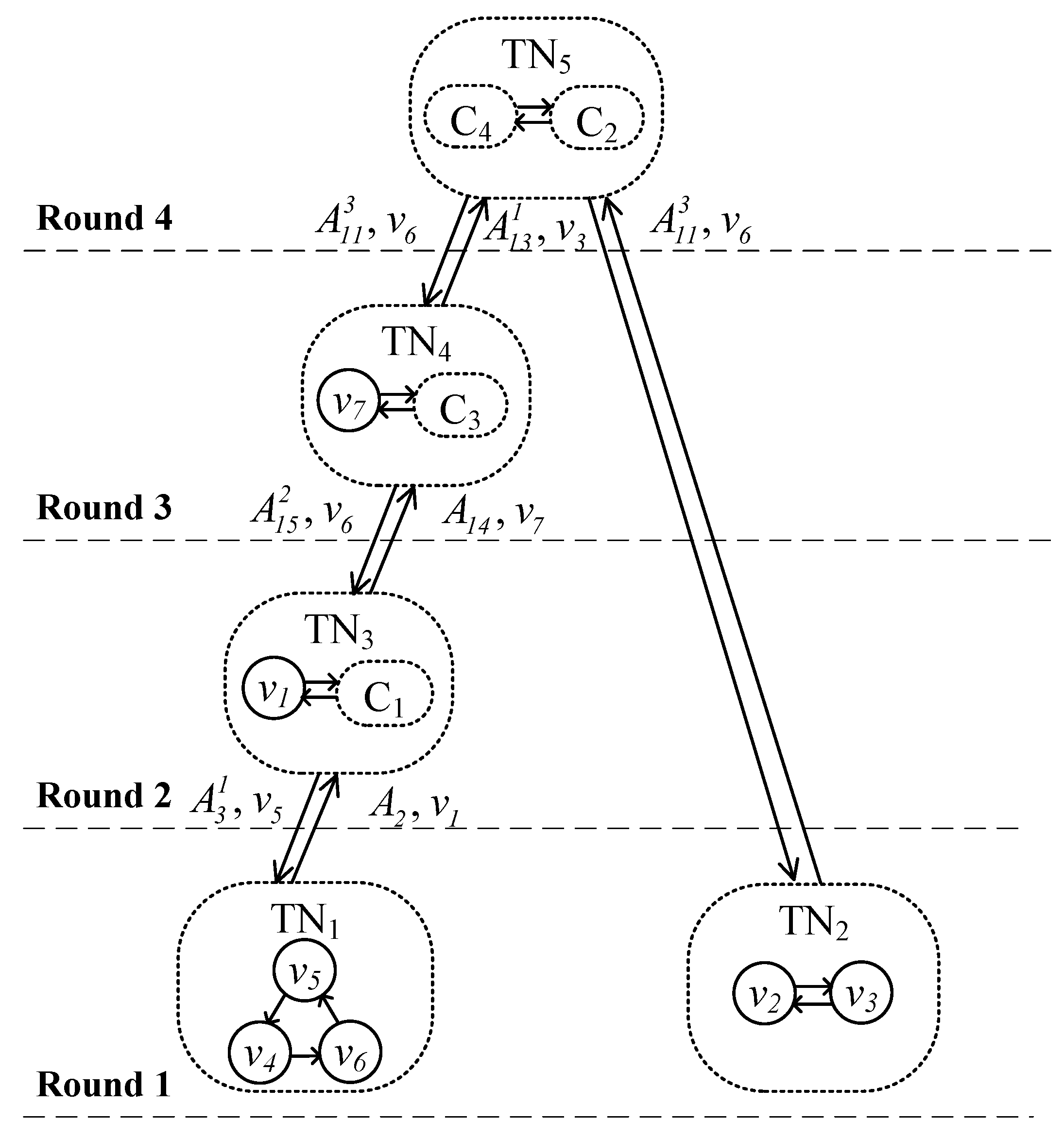
Example 5. 

In Figure 5, we show the hierarchical tree of Example 4. Furthermore, we mark the linking edge and linking vertex between the child tree node and its parent. In the first round, we detect cycles $c_1=\{v_4,v_5,v_6\}$ and $c_2=\{v_2,v_3\}$. Then, we build tree node $T{N}_1$ and $T{N}_2$. In the second round, we detect cycle $c_3=\{v_1,c_1\}$. Furthermore, we build tree node $T{N}_3$. $c_1$ is a member of $T{N}_3$, the in-edge of $c_1$ incident $c_1$ on $v_5$ and the out-edge of $c_1$ is $A_2$. Therefore, we link $T{N}_1$ with $T{N}_3$ by linking edges $A_3^1$ and $A_2$ and linking vertices $v_5$ and $v_1$. Repeat this procedure on each tree node and we have H in Figure 5.

5.2. Expansion

Now that we have all the potential edges of $DMST$ at an arbitrary root in graph G in H, we need to find all the edges of T for any given root. However, the vertices and cycles are in a hierarchical index structure. We have to design an order of expansion so that we can recover the $DMST$ of any given root and ensure correctness.

Suppose there is only one tree node in the hierarchical tree. For any given root r, we just need to delete the in-edge of r, break the cycle, and find the $DMST$ rooted at r. For more tree nodes in H, the cycles are organized hierarchically. We can expand r following Lemma 1. We first locate the tree node of r, $TN\left(r\right)$, then break $TN\left(r\right)$ as we do with only one tree node. If $TN\left(r\right)$ is not the root node of the hierarchical tree, we find the parent tree nodes of $TN\left(r\right)$ along the linking edges and expand each parent tree node by regarding the linking vertex as the new root. If $TN\left(r\right)$ has child tree nodes, we find its child tree nodes along the linking edges and expand each child tree node by regarding the linking vertices as the new root.

Example 6. 

Given root $v_1$, we first locate its tree node $TN\left(v_1\right)$, delete $A_2$ and break $c_1$ and delete $A_8$. Then $c_3$ in $T{N}_4$ is the root in round 3, and we delete $A_{15}^2$. Then $c_4$ in $T{N}_5$ is the root in round 4, we delete $A_{11}^3$, break $c_2$ and delete $A_4$. Now we have $T_{v_1}$ of total weight 29.

Here is how we expand with reference to the index in detail:

Delete the in-edge of the root. For any given root vertex r in H, we first locate the tree node $TN\left(r\right)$ it is in. $TN\left(r\right)$ is a cycle. Starting from r, we traverse along the out-edges of each vertex in the cycle and delete the in-edge of the root r in the cycle to break the cycle.

Locate new roots. In the traversing procedure in $TN\left(r\right)$, when meeting a linking edge $e_l$ and linking vertex $v_l$, we treat $v_l$ as the new root in the child tree node $TN\left(v_l\right)$ and repeat the procedure in $TN\left(v_l\right)$. Then we go up to the parent of $TN\left(r\right)$ along the linking edge, treat the linking vertex as the new root, and repeat the procedure.

In Algorithm 2, starting from root v and tree node $t{n}_v$ (line 3), we first break the cycle by removing the in-edge of root vertex v (line 5). We put all the linking edges in $TN\left(v\right)$ in queue Q (line 8) and add them to T (line 9). If $TN\left(v\right)$ is not the root node (line 10), we put its parent tree node $TN\left(pv\right)$ and its linking vertex $v^{\prime }$ to queue Q (line 12). From the view of tree H, in each round we put all its neighbors, its child nodes, and parent node in the queue. It traverses the tree in a BFS manner.

Algorithm 2: Expansion $(H,r)$

For the $FindCycle$ procedure, shown in Algorithm 3, we use all the minimum in-edges $MI$ found this round and return the set of cycles. For each $v\in MI$ (line 2), we start traversing backward along the minimum in-edge of v, and dye the vertices met with color i (lines 13–14). If we encounter any vertex with the same color of i, then a cycle is found (lines 4–5). We put all the vertices of color i in the cycle $c_i$ (lines 7–10). Then we start from the next vertex in $MI$ until all the vertices in $MI$ are visited.

Algorithm 3: FindCycles $\left(MI\right)$

Example 7. 

For the original graph in Figure 1, we have the hierarchical tree H in Figure 5. We show how we search for ${\mathcal{T}}_{v_1}$ in the expansion phase. For root $v_1$, we add $A_3$ to T then we enqueue $\{T{N}_1,v_5\}$ and $\{T{N}_4,C_3\}$. Next round, for $\{T{N}_1,v_5\}$ we add $A_7$ and $A_{10}$ to T. Next round, for $\{T{N}_4,C_3\}$ we add $A_{14}$ to T then enqueue $\{T{N}_5,C_4\}$. Next round, for $\{T{N}_5,C_4\}$ we add $A_{13}$ to T and enqueue $\{T{N}_2,v_3\}$. Next round, for $\{T{N}_2,v_3\}$ we add $A_5$ to T. By now, we have obtained the $DMST$${\mathcal{T}}_{v_1}$ at root $v_1$.

Theorem 1. 

Algorithm 2 correctly computes the $DMST$ at given root r.

Proof. 

Firstly, our algorithm traverses the hierarchical tree in a BFS manner. If BFS can traverse the entire tree, so can our algorithm. Therefore, our algorithm breaks all the cycles and returns a tree. Secondly, we prove this by contradiction. Suppose our algorithm returns $T^{\prime }$ larger than T. This indicates that some edges of $T^{\prime }$ are not the minimum in-edges of vertices in $T^{\prime }$. It contradicts the fact that edges in H are the minimum in-edge related to each vertex found in each round in H. Therefore, our algorithm correctly computes the $DMST$ at root r.    □

Theorem 2. 

The query time of the expansion phase is $O\left(n\right)$.

Proof. 

There are at most $n-1$ cycles and at most $2(n-1)$ edges in H. We have to delete at most $n-1$ edges and add at most $n-1$ edges to obtain $DMST$. We traverse H in $O\left(n\right)$ time and add edges to T in $O(n-1)$ time. Therefore, the query time of the expansion phase is $O\left(n\right)$.    □

5.3. Hierarchical Tree Construction

The construction of the hierarchical tree is detailed as follows:

Contract the root. We do not specifically exclude the root vertex from the contraction phase. As we assume the graph is strongly connected, the graph will finally contract to a single vertex. The algorithm still generates the correct result as proved in Lemma 1.

Store potential tree edges. To reuse the edges and cycles in the contraction phase, we store all the edges that will be tree edges of any root. We store every edge of each cycle when we contract, and delete the edges that will not be in the tree when we query.

For each round of contraction, we select minimum in-edges of each vertex, find cycles, contract cycles into vertices and update corresponding in-edges in a recursive manner. The cycles are naturally hierarchical (Observation 1). We, therefore, build a hierarchical tree H with each tree node corresponding to a cycle. Then by linking child tree nodes and their parent tree nodes, we construct a tree H of cycles. Here, we build the hierarchical tree.

Find cycles. For round i, we first choose the minimum in-edge of each vertex, then we find cycles of this round.

Build the tree node. The cycles found in round 1 will be leaf nodes. For round i, we store all vertices in cycle $c_i\subset C$ found this round into tree node $T{N}_j$. Furthermore, we contract the cycle to a new vertex.

Build Tree H. For round i, if $T{N}_j$ is not a leaf node, we link it with its child nodes by linking edges with linking vertices. Finally, we build the hierarchical tree of cycles H.

We introduce our contraction algorithm in Algorithm 4. For each round, we find minimum in-edges incident on v and find cycles. If no cycle is found this round, we have contracted the graph into a single vertex (lines 3–8). For every in-edge whose head is a vertex in cycles and a tail out of cycles found this round, we update their cost and add them to the new edge set $E^{\prime }$ (lines 9–11). After that, we contract cycles into a vertex and add it to the new vertex set $V^{\prime }$ (lines 12–13). We then add the vertices not in cycles and their minimum in-edge to the new graph $G^{\prime }$, update the graph G, and put cycles to corresponding tree nodes (lines 14–18). Finally, the algorithm returns the hierarchical tree of the cycles.

Lemma 3. 

We have to contract at most $n-1$ cycles in the directed graph G.

Proof. 

Lemma 3 is true for $\left|V\right|=1$. Suppose it is true for $\left|V\right|=n-1$, and at most $n-2$ cycles are contracted. When $\left|V\right|=n$ and $V=\{v_1,...,v_{n-1},v_n\}$, we first pick any $n-1$ vertices $V^{\prime }=\{v_1,...,v_{n-1}\}$. $V^{\prime }$ can contract to a vertex $v^{\prime }$, and at most $n-2$ cycles are contracted. As the graph will finally contract to a single vertex, the contracted vertex $v^{\prime }$ and the left vertex $v_n$ can contract to a cycle. Therefore, Lemma 3 holds.    □

Lemma 4. 

We have to store at most $2(n-1)$ potential tree edges in the hierarchical tree H.

Proof. 

According to Lemma 3, there will be at most $n-1$ cycles in the directed graph. Each cycle has at least two edges. Therefore, we need to store at most $2(n-1)$ edges.    □

Lemma 5. 

We have to delete at most $n-1$ edges from the hierarchical tree H to obtain $DMST$.

Proof. 

For the directed graph G with n vertices, the $DMST$ contains $n-1$ edges. The $DMST$ contains n vertices each vertex has an in-edge except the root vertex, and the $DMST$ has $n-1$ edges. According to Lemma 4, we store at most $2(n-1)$ edges in the hierarchical tree H, therefore we have to delete at most $n-1$ edges from H.    □

Algorithm 4: Contraction $\left(G\right)$

6. Batch Query

In this section, we process a sequence of query vertices in a batch by utilizing the unaffected edges of different query vertices. Furthermore, we discuss the query scheduling to minimize the total query cost.

6.1. Batch Query Processing

For a sequence of query vertices, the two distinct query vertices may share many common edges. If we process each vertex independently, we have to break all the cycles and delete the edges for each query, which is costly.

Example 8. 

In Figure 5, for query vertex $v_4$, ${\mathcal{T}}_{v_4}$ and next query vertex $v_5$, ${\mathcal{T}}_{v_5}$. The difference between ${\mathcal{T}}_{v_4}$ and ${\mathcal{T}}_{v_5}$ are only the in-edges of $v_4$ and $v_5$. Actually, to obtain ${\mathcal{T}}_{v_5}$, we only need to add $A_7$ and delete $A_8$ from ${\mathcal{T}}_{v_4}$.

Observation 3. 

We derive this observation from Observation 2 and the expansion phase. For two distinct query vertices $q_i$ and $q_{i+1}$, given a cycle c they both have to break in their expansion phase, we identify the new roots $v_i,v_j\in c$, $j\ne i$ for them. $q_i$ breaks the cycle c at vertex $v_i$, the in-edge of $v_i$ will be deleted. $q_{i+1}$ breaks the cycle at $v_j$ and delete its in-edge. The edge difference of $q_i$ and $q_{i+1}$ breaking cycle c are the in-edges of $v_i$ and $v_j$ in cycle c.

From the child tree node to the parent tree node, there is a linking vertex, and we treat it as the new root to break the parent tree node in the expansion phase if there is a query vertex in the child tree node. Therefore, different vertices in the parent tree node are related to different child tree nodes. Furthermore, vertices in the ancestor tree node are related to a subtree of child nodes.

Lemma 6. 

Given $q_i$, ${\mathcal{T}}_{q_i}$, $q_{i+1}$, ${\mathcal{T}}_{q_{i+1}}$, the difference between ${\mathcal{T}}_{q_i}$ and ${\mathcal{T}}_{q_{i+1}}$ are in the subtree rooted at $q_i$ and $q_{i+1}$’s Least Common Ancestors (LCA) in the hierarchical tree H.

Proof. 

We prove this by contradiction. $TN\left(q_i\right)$ and $TN\left(q_{i+1}\right)$ have linking vertices in their parent tree nodes. In their LCA tree node $T{N}_{lca}$, their parent tree nodes have different linking vertices $v_i$ and $v_{i+1}$ related to $q_i$ and $q_{i+1}$ as the new roots. Suppose parent of $T{N}_{lca}$ is $T{N}_p$, the linking vertex from $T{N}_{lca}$ to $T{N}_p$ is $v_{lca}\in T{N}_p$. Suppose an arbitrary edge with a head vertex $v_a\ne v_{lca}$ and a tail vertex $v_b$ in $T{N}_p$ is affected. Based on Observation 3, the in-edge of $v_a$ and in-edge of $v_{lca}$ are affected. It indicates that there is one query vertex from a subtree of $T{N}_p$ related to $v_a$ and one query vertex from a subtree of $T{N}_p$ related to $v_{lca}$, which contradicts that both $q_i$ and $q_{i+1}$ are in the subtree related to $v_{lca}$, and no query vertex is related to $v_a$.    □

From Lemma 6, we reduce the edges to be updated from the entire $DMST$ to the subtree of the $DMST$s of two distinct query vertices. Furthermore, we have to identify the cycles and edges to be updated. Based on Observation 3, only two edges are affected in each cycle related to the query vertex. Therefore, we only need to decide on the affected cycles and find the root vertex related to the query vertices when we break the cycles.

We identify the affected cycles by traversing along the linking edges and decide the new roots in each cycle by linking vertices. For two query vertices $q_i,q_{i+1}$, we discuss the update from $q_{i+1}$ to $q_i$ as the operations are symmetric. If $q_i,q_{i+1}$ are in the same tree node, we just update their in-edges. Otherwise, in their LCA tree node $T{N}_{lca}$, we find the in-edge $A_{lca}$ of the new root related to $q_i$ in $T{N}_{lca}$, and identify the $head\left(A_{lca}\right)$ as the new root in $TN\left(head\left(A_{lca}\right)\right)$. Then we repeat the above procedure with $q_i$ and $head\left(A_{lca}\right)$. Finally, we will identify all the affected edges and cycles and report the correct result.

We introduce our batch query algorithm in Algorithm 5. We find the LCA of two query vertices and their corresponding vertices in their LCA (line 3). Then we update the affected edges in their LCA cycle (lines 4–7). We locate the new roots in the next affected cycles (lines 8–9). Furthermore, we process the affected edges of cycles in a recursive way until all affected cycles are traversed (lines 10–13).

Algorithm 5: BatchExpansion $(T,q_i,q_{i+1})$

Example 9. 

In Figure 5, for query vertex $v_7$ and next query vertex $v_1$, the LCA of them is $T{N}_4$. We first update the edges from $v_1$ to $v_7$. In $T{N}_4$, $v_7$ and $C_3$ are affected. $A_{14}$ is added and $A_{15}$ is deleted. $v_7$ and $head\left(A_{14}\right)=v_7$ are in the same cycle, and the procedure terminates. Then we update the edges from $v_7$ to $v_1$. The LCA of $head\left(A_{15}\right)=v_6$ and $v_1$ is $T{N}_3$. In $T{N}_3$, $v_1$ and $C_1$ are affected. $A_3$ is added and $A_2$ is deleted. $v_1$ and $head\left(A_2\right)=v_1$ are in the same cycle, and the procedure terminates. The LCA of $head\left(A_{15}\right)=v_6$ and $head\left(A_3\right)=v_5$ is $T{N}_1$. In $T{N}_1$, $v_5$ and $v_6$ are affected. $A_{10}$ is added and $A_8$ is deleted. By now, we correctly update edges and obtain ${\mathcal{T}}_{v_1}$ from ${\mathcal{T}}_{v_7}$.

Theorem 3. 

Algorithm 5 correctly update all the changed edges.

Proof. 

Based on Observation 3 and Lemma 6, we need to process all affected edges of the cycles contained in the sub-tree of the LCA. Algorithm 5 first finds the LCA of two query vertices and then traverses all the cycles in a recursive way. Therefore, all the cycles of the sub-tree and the affected edges are correctly updated. □

Theorem 4. 

Algorithm 5 runs in worst-case $O\left(n\right)$ time complexity.

Proof. 

We locate LCA in $O\left(1\right)$ time [21]. Suppose the LCA of $q_i$ and $q_{i+1}$ is the root of H, and there are only two edges in each child cycle. Therefore, the worst-case time complexity is the same as re-running a single query by Algorithm 2. □

6.2. Query Scheduling

An optimal query scheduling can minimize the total cost of batch queries. However, obtaining an optimal order of query sequence is costly.

Instead, we adopt a simple heuristic method of query scheduling. We order the query sequence by its proximity. The closer the two vertices in the tree nodes of H, the lower the cost of querying the next root vertex. We traverse H post-order and label the tree node with the traversing order. Then we sort the query sequence by their corresponding traverse order. The total cost is $O(n+klogk)$ time complexity and $O\left(n\right)$ space complexity, where k is the size of the query sequence and n is the number of cycles. We evaluate the post-order query scheduling in the experiment.

Theorem 5. 

Post-order query scheduling is a two-approximation of optimal query scheduling.

Proof. 

Suppose the optimal sequence of query scheduling is $S=\{q_1,q_2,\cdots ,q_{k-1},q_k\}$, and they correspondent to tree nodes $TN\left(q_1\right)$, $TN\left(q_2\right)$, ⋯, $TN\left(q_{k-1}\right)$ and $TN\left(q_K\right)$. The optimal scheduling is a path on H that starts from $TN\left(q_1\right)$ and ends at $TN\left(q_k\right)$. We denote the path as R. For a Steiner Tree that spans all the corresponding tree nodes in S, we denote the minimum one as $MST$. Both R and $MST$ are connected graphs while $MST$ is the minimum one. Therefore, we have $R\ge MST$. For the post-order traverse on the $MST$, denoted as $PO$, edges will be visited at most twice. So we have $MST\ge \frac{1}{2}PO$. Therefore, we have $R\ge \frac{1}{2}PO$, and the post-order query scheduling is a two-approximation of optimal scheduling. □

7. Experiment

All algorithms were implemented in C++ and compiled with GNU GCC 4.4.7. All experiments were conducted on a machine with an Intel Xeon 2.8GHz CPU and 256 GB main memory running Linux (Red Hat Linux 4.4.7, 64bit).

In

Table 2. Dataset.

Name	Abbrv	Type	#Vertices	#Edges
US airports	UA	Infrastructure Network	1402	28,032
p2p-Gnutella30	PG	Computer Network	13,375	37,942
soc-Epinions1	SE	Online Social Network	32,223	443,506
wiki-Talk	WT	Communication Network	111,881	1,477,893
web-BerkStan	WB	Hyperlink Network	334,856	4,523,219
soc-Pokec	SP	Online Social Network	1,304,536	29,183,654

, we use the open source direct graph dataset from SNAP (https://snap.stanford.edu/data/, last time accessed on 19 February 2023) and KONECT (http://konect.cc/, last time accessed on 19 February 2023). We extracted the Strongly Connected Component from these directed datasets and removed all the self-loops. If the dataset was unweighted, we assigned random weights to the edges. We randomly generated 1000 queries and show the average cost as query time.

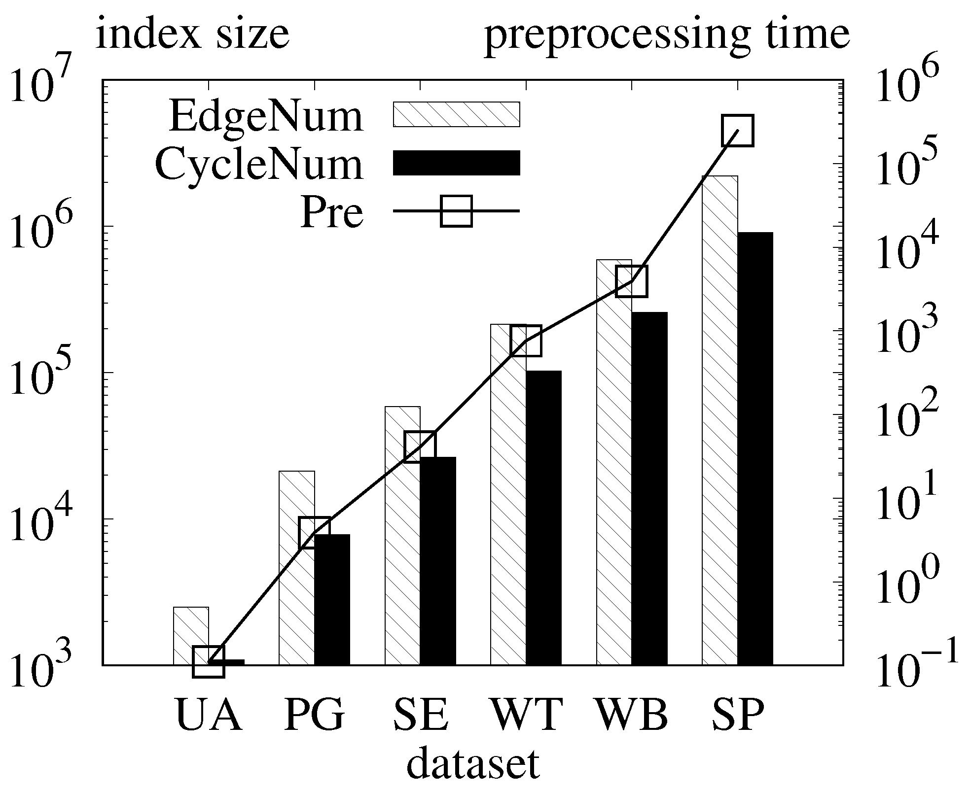
Exp-1. Index size and indexing time. We show the number of edges “EdgeNum” in the hierarchical tree of each dataset, the number of cycles “CycleNum”, and the preprocessing time “Pre” Figure 6. The number of edges and cycles in the hierarchical tree $T_H$ grows linearly with the size of the graph. For example, for dataset $UA$, the number of edges is 2492, and the number of cycles is 1091, and for dataset SP, the number of edges in the tree is 2,210,189, and the number of cycles in the tree is 905,654.

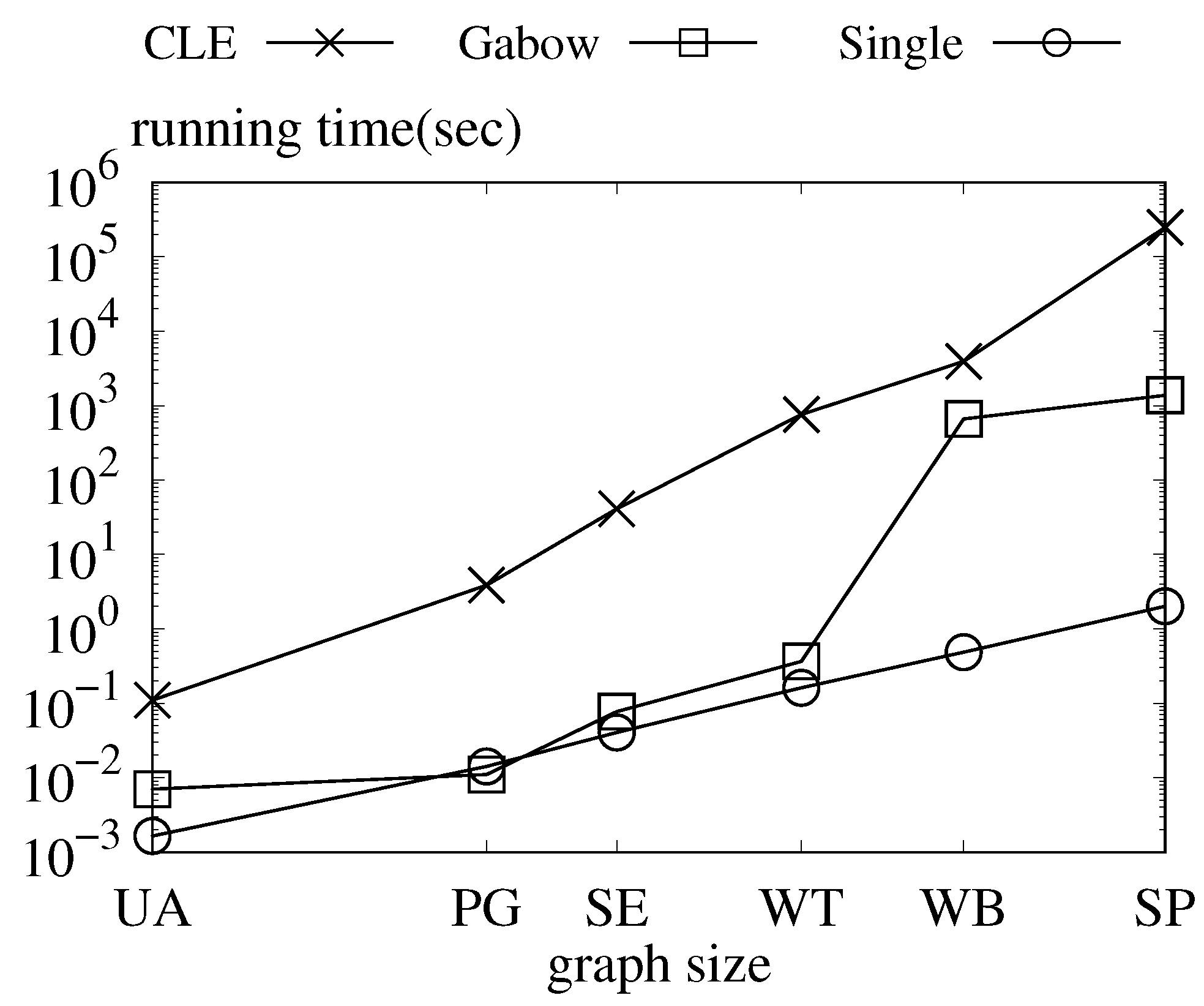
Exp-2. Compare the single query time. In this experiment, we show the single query time of Chu-Liu and Edmonds’ as “CLE”. We also show the single query time of Gabow [20] implemented with a Fibonacci heap as “Gabow”. Furthermore, we show the average single query time of ours as “single” in Figure 7. The processing time of $CLE$ increases dramatically as the size of datasets increases, owing to the $O\left(mn\right)$ time complexity. Though $Gabow$ shows good performance in relatively small graphs, it suffers from an increasing number of edges when the graph size grows. Meanwhile, our $single$ query time is linear to the growth of graph size because of $O\left(n\right)$ time complexity. For dataset $UA$, $CLE$’s single query time is 0.1100 s. $Gabow$’s single query time is 0.0070 s. Our single query time is 0.0016 s. For dataset $PG$, $CLE$’s single query time is 3.8600 s. $Gabow$’s single query time is 0.01100 s. Our single query time is $0.0142$. For dataset $SE$, $CLE$’s single query time is 41.0300 s. $Gabow$’s single query time is 0.0770 s. Our single query time is 0.04060s. For dataset $WT$, $CLE$’s single query time is $706.92$. $Gabow$’s single query time is 0.3640 s. Our single query time is 0.1607 s. For dataset $WB$, $CLE$’s single query time is 3918.85 s. $Gabow$’s single query time is 660.6230 s. Our single query time is 0.4851 s. For dataset $SP$, $CLE$’s single query time is 251,089 s. $Gabow$’s single query time is 1371.1320s. Our single query time is 2.0151 s. We can see that our single query time shows better performance than the online ones.

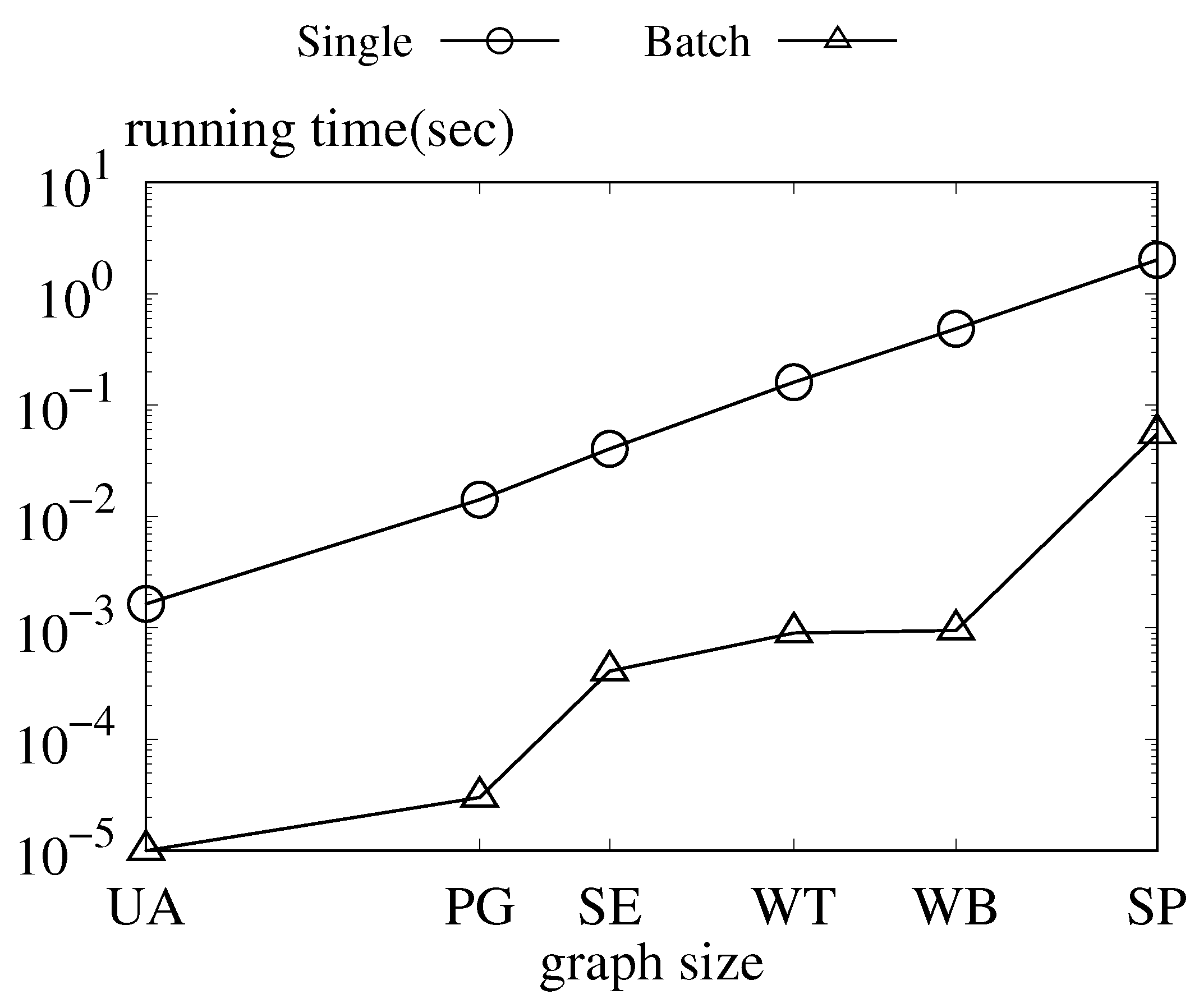
Exp-3. Compare single and batch query time. In this experiment, we compare the performance of our single query and batch query algorithms. The single query time grows linearly with the increase in the graph size. In the meantime, the batch query time is affected by the size and structure of the graph. As the batch query is related to the size of cycles of each dataset, more cycles in the graph indicate a greater time cost in query time. Though a larger graph size indicates more cycles, the number of cycles is related to the structure of the graph. Despite this, the batch query time is at least an order of magnitude faster than the single query.

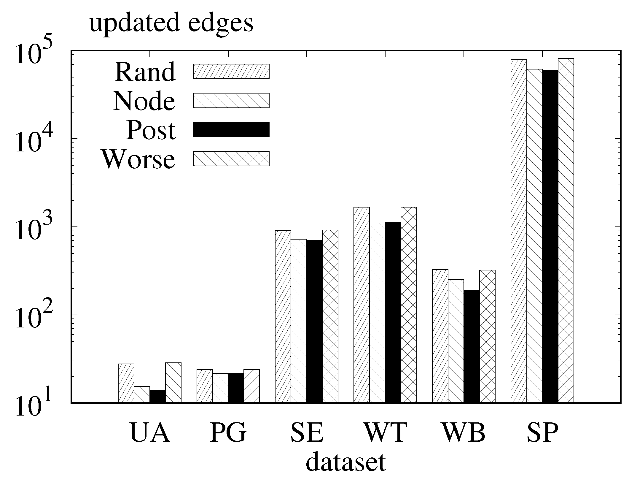
Exp-4. Query scheduling of batch query. To evaluate the effect of query scheduling on the batch query. We conduct our experiment on different order schemes. We show the average number of updated edges of the random order as “Rand”, the average number of updated edges of scheduling by the node ID as “Node”, and the average number of updated edges of post-order traverse as “Post”. Furthermore, we construct a relatively worse case by selecting the next query vertex with less proximity to the previous one. We denote such a worse case as “Worse”. The results are shown in Figure 8. For all the datasets, random query scheduling updates a similar number of edges as the constructed relatively worse case. Furthermore, post-order scheduling performs slightly better than the sequence ordered by node ID. Both the post-order and node ID order are better than random order and the worse case. The good performance of scheduling by the node ID shows the close relationship between cycles during the construction of hierarchical tree H (Figure 9).

8. Conclusions

We propose an indexed approach to answer the $DirectedMinimumSpanningTree$ query of any root. We first pre-process the directed graph in $O\left(mn\right)$ time. In the procedure, we build a hierarchical tree that stores all the edges of potential $DMST$ with a space complexity of $O\left(n\right)$. In the expansion phase, starting from the given root, we traverse all of its out-edges on H in a BFS manner to obtain the $DMST$. Then, we propose a batch expansion algorithm by utilizing the shared edges of two query vertices. The time complexity of both expansion algorithms is $O\left(n\right)$.