Convolution, Correlation, and Uncertainty Principles for the Quaternion Offset Linear Canonical Transform

Abstract

Quaternion Fourier transform (QFT) has gained significant attention in recent years due to its effectiveness in analyzing multi-dimensional signals and images. This article introduces two-dimensional (2D) right-sided quaternion offset linear canonical transform (QOLCT), which is the most general form of QFT with additional free parameters. We explore the properties of 2D right-sided QOLCT, including inversion and Parseval formulas, besides its relationship with other transforms. We also examine the convolution and correlation theorems of 2D right-sided QOLCT, followed by several uncertainty principles. Additionally, we present an illustrative example of the proposed transform, demonstrating its graphical representation of a given signal and its transformed signal. Finally, we demonstrate an application of QOLCT, where it can be utilized to generalize the treatment of swept-frequency filters.

1. Introduction

An expansion of two-dimensional (2D) Fourier transform (FT) in Hamiltonian quaternion algebra is called 2D quaternion Fourier transform (QFT) [1,2]. QFT plays a crucial role in representing 2D quaternion-valued signals, which is an essential tool for multi-channel and multi-dimensional space. Because of the non-commutative property of multiplication of quaternion algebra, there are mainly three types of quaternion integral transforms: two-sided, left-sided, and right-sided [1]. The simplicity of the Hamiltonian algebra representation of signals, where red, green, and blue channels are controlled simultaneously, has led to diverse applications of QFTs in signal detection, steganography systems, speech recognition, and color image processing [3,4,5,6,7], as well as in partial differential systems and mathematical statistics [8,9]. Over the last few years, there has been a growing interest in establishing the various properties of quaternion-valued FTs, including duality, sampling, product, convolution and correlation, uncertainty principle, etc. [10,11,12,13,14,15,16]. Furthermore, QFT has been generalized to quaternion fractional Fourier and quaternion linear canonical domains [17,18,19,20,21,22], and their associated localized transforms have been investigated in [23,24,25]. The collective findings of these studies have contributed significantly to the elucidation of the underlying principles governing quaternion-valued FTs and their potential utility across a broad spectrum of disciplines.

Offset linear canonical transform (OLCT) is a six-parameter $A=\left(a,b,c,d,\tau ,\eta \right)$ class of linear integral transforms including the Fourier, fractional Fourier, and linear canonical transforms (LCT) [26,27,28]. OLCT is a powerful tool that not only generalizes the classical transforms but also provides better flexibility in its applicability in signal processing, optics, and many other areas [29,30,31,32,33]. When different matrix $A$ parameters are considered, OLCT converts to its special cases, thus enabling deeper insights into its special cases. The applications of OLCT are similar to LCT, but they are more general and flexible than LCT. It is proven that OLCT is not just a generalization of LCT, but able more than LCT. Although significant progress has been made in investigating the fundamental theories and properties of OLCT in recent years, a few attempts have been made to extend OLCT to quaternion domains [34,35,36,37,38]. However, a formal extension of right-sided OLCT to quaternion domains remains unknown. The development of the quaternion offset linear canonical transform (QOLCT) provides a pathway towards a broader understanding of its special cases and is worth attention.

The purpose of this article is to define the 2D right-sided QOLCT. Importantly, by introducing the relationship between right and left-sided QOLCT, we show that right-sided QOLCT is easily converted to left-sided QOLCT. All research on right-sided QOLCT is true for left-sided QOLCT. Furthermore, we illustrate right-sided QOLCT relationships with other transforms and obtain different basic properties, such as linearity, translation, modulation, parity, and others. Moreover, using the proposed Parseval formula, we obtain an inversion formula for right-sided QOLCT. Furthermore, we investigate the convolution and correlation theorems of right-sided QOLCT, which is not reported yet in the open literature and is vital for QOLCT applications. In addition, we establish Heisenberg-Pauli-Weyl and Pitt’s inequalities for right-sided QOLCT. After that, using a sharp form of Pitt’s inequality and the Parseval formula, we derive the logarithmic uncertainty principle for the 2D right-sided QOLCT, which is a general form of the Heisenberg uncertainty principle. Then, we give an example of QOLCT, where we graphically represent the given signal and the transformed signal. Moreover, we show an application of the proposed transform, where QOLCT generalizes the treatment of swept-frequency filters. Also, we discuss the advantages of the QOLCT in optical systems compared to previously known quaternion-valued FT-related integral transforms. Finally, we discuss why such transforms should be studied using color image processing as an example.

The article is organized as follows: In Section 2, we review the quaternion algebra and present some notations. In Section 3, we consider the 2D right-sided QOLCT definition, together with its properties and relationships. In Section 4, the concepts of convolution and correlation theorems are introduced. In Section 5, the uncertainty principles are described. Section 6 shows the QOLCT example and application. In Section 7, future potential applications are discussed. Finally, this article is concluded in Section 8.

2. Preliminaries

2.1. Quaternion Algebra

Quaternion, denoted by $ℍ,$ is an extension of a complex field $ℂ$ to 4D algebra, introduced by Hamilton in 1843. Since it has been used to represent the rotations of objects in 3D space and become an active area of research with different applications in signal processing, applied mathematics, and engineering. Quaternion is a linear combination of a real scalar and three orthogonal imaginary elements $i, j, k$ with real coefficients, written as

$$ℍ=\left\{f=q_0+i{q}_1+j{q}_2+k{q}_3\right.;\left.q_0,q_1,q_2,q_3\in ℝ\right\},$$

here the three different imaginary elements obey Hamiltonian multiplication rules

$$i^2=j^2=k^2=ijk=-1, ij=-ji=k, jk=-kj=i, ki=-ik=j.$$

(1)

It is obvious from (1) that the quaternion multiplication is not commutative.

Every quaternion $f$ has a quaternion conjugate

$$\overline{f}=q_0-i{q}_1-j{q}_2-k{q}_3.$$

(2)

An anti-involution property takes a form

$$\overline{fg}=\overline{g}\overline{f},\overline{f+g}=\overline{f}+\overline{g},\stackrel{=}{f}=f.$$

(3)

From (2), the norm of $f\in ℍ$ can be defined as the multiplication of a quaternion $f$ with the conjugate $\overline{f}$ as

$${‖f‖}_{L^2}=\sqrt{f\overline{f}}=\sqrt{q_0^2+q_1^2+q_2^2+q_3^2}.$$

Any quaternion can be represented by

$$f=\left(q_0+i{q}_1\right)+j\left(q_2-i{q}_3\right)=f_1+j \overline{f_2},$$

where $f_1,f_2\in ℂ$ are two complex numbers.

The inner product of any two quaternions $f,g\in ℍ$ is defined by

$${〈f,g〉}_{L^2}=f\overline{g}=\left(f_1\overline{g_1}+\overline{f_2}\overline{g_2}\right)-j\left(f_1\overline{g_2}-\overline{f_2}\overline{g_1}\right).$$

Throughout this article, from now and on, we will use the subsequent real vector notations

$$\mathbf{z}=\left(z_1,z_2\right)\in {ℝ}^2,{\left|\mathbf{z}\right|}^2=z_1^2+z_2^2,f\left(\mathbf{z}\right)=f\left(z_1,z_2\right),d\mathbf{z}=d{z}_{1}d{z}_2.$$

The quaternion-valued function can be written as

$$f(\mathbf{z})=f_0(\mathbf{z})+\underset{¯}{f}(\mathbf{z}),$$

where $f_0(\mathbf{z})$ is the real scalar part and $\underset{¯}{f}(\mathbf{z})=i{f}_1(\mathbf{z})+j{f}_2(\mathbf{z})+k{f}_3(\mathbf{z})$ is the vector (pure) part of $f(\mathbf{z})$.

It is easy to determine that the quaternion-valued function $f:{ℝ}^2\to ℍ$ can be decomposed as $f\left(\mathbf{z}\right)=f_1 \left(\mathbf{z}\right)+j f_2\left(\mathbf{z}\right),$ where $f_1, f_2$ are complex-valued functions.

Let us denote $L^2\left({ℝ}^2,ℍ\right),$ the space of all quaternion-valued functions $f$ satisfying

$${‖f‖}_2={\left\{{{\displaystyle {\int }_{{ℝ}^2}\left|f\left(\mathbf{z}\right)\right|}}^{2}d\mathbf{z}\right\}}^{1/2}<\infty .$$

The norm of $L^2\left({ℝ}^2,ℍ\right)$ is obtained from the inner product of the quaternion-valued functions $f\left(\mathbf{z}\right)=f_1+j f_2$ and $g\left(\mathbf{z}\right)=g_1+j g_2$ as

$${{〈f,g〉}_{}}_{L^2({\mathbb{R}}^2,\mathbb{H})}={\int }_{{\mathbb{R}}^2}f\left(\mathbf{z}\right)\overline{g\left(\mathbf{z}\right)}d\mathbf{z}.$$

(4)

Consequently, the quaternionic Cauchy-Schwarz inequality for any $f,g\in L^2({ℝ}^2,ℍ)$ can be obtained as

$$\left|{〈f,g〉}_{L^2({\mathbb{R}}^2,\mathbb{H})}\right|\le {∥f∥}_{L^2({\mathbb{R}}^2,\mathbb{H})}{∥g∥}_{L^2({\mathbb{R}}^2,\mathbb{H})}.$$

(5)

2.2. Existing Quaternion Transforms

This subsection will recall the 2D right-sided QFT and quaternion linear canonical transform (QLCT) definitions that are used in the subsequent sections.

Definition 1.

(2D right-sided QFT) [1]. For any quaternion-valued signal $f\in L^2\left({ℝ}^2,ℍ\right),$ the 2D right-sided QFT (denoted by ${}_R\mathcal{F}{}^{ℍ}$) is given as

$${}_R\mathcal{F}{}^{ℍ,\mu }\left\{f\left(\mathbf{z}\right)\right\}\left(\mathbf{v}\right)={\displaystyle {\int }_{{ℝ}^2}f\left(\mathbf{z}\right)e^{-\mu z_1{v}_1}{e}^{-\mu z_2{v}_2}d\mathbf{z}},$$

(6)

where $e^{-\mu z_1{v}_1}{e}^{-\mu z_2{v}_2}$ is a quaternion Fourier kernel, and $\frac{i+j+k}{\sqrt{3}}=\mu \in ℍ$ is a pure unit quaternion, such as ${\mu }^2=-1.$

Definition 2.

(2D right-sided QLCT) [8,9]. Let $A_n=\left(a_n,b_n,c_n,d_n\right)$ with real parameters $a_n,b_n,c_n,d_n\in ℝ,$ such as $a_n{d}_n-b_n{c}_n=1,$ $n=1,2.$ For any quaternion-valued signal $f\in L^2\left({ℝ}^2,ℍ\right)$ the 2D right-sided QLCT (denoted by ${}_R{\mathcal{L}}_{A_1,A_2}^{\mathbb{H},\mu }$) is given as

$${}_R{\mathcal{L}}_{A_1,A_2}^{\mathbb{H},\mu }\left\{f\left(\mathbf{z}\right)\right\}\left(\mathbf{v}\right)={\int }_{{\mathbb{R}}^2}f\left(\mathbf{z}\right)K_{A_1}\left(z_1,v_1\right)K_{A_2}\left(z_2,v_2\right)d\mathbf{z},$$

where $K_{A_1}\left(z_1,v_1\right) K_{A_2}\left(z_2,v_2\right)$ is a quaternion linear canonical kernel

$$K_{A_n}\left(z_n,v_n\right)=\frac{1}{\sqrt{2\pi b_n\mu }}{e}^{\mu \frac{1}{2b_n}\left(a_n{z}_n^2-2z_n{v}_n+d_n{v}_n^2\right)},b_n\ne 0,$$

with the polar form of $1/\sqrt{\mu }=e^{-\mu \frac{\pi }{4}}.$ It is clear that

$$e^{-\mu \frac{\pi }{4}}=e^{\mu \frac{\pi }{2}\left(-\frac{1}{2}\right)}={\left(\cos \frac{\pi }{2}+\mu \sin \frac{\pi }{2}\right)}^{-\frac{1}{2}}={\mu }^{-\frac{1}{2}}.$$

For a more precise understanding of quaternion integral transforms, one can refer to [1,17,20,23,24,34].

3. Right-Sided Quaternion Offset Linear Canonical Transform (QOLCT)

Motivated by the importance of quaternion algebra in signal/image processing and the flexibility of OLCT, we introduce the 2D right-sided and left-sided QOLCTs, then list their special cases. After then, we show the relationship between right and left-sided QOLCTs, and present QOLCT relationships with QFT and QLCT. At the end of this section, different properties, including linearity, additivity, translation, modulation, and parity, are listed. Notably, Parseval and inversion formulas are depicted.

3.1. Definitions

We obtain the 2D right-sided QOLCT by replacing the kernel of OLCT with the quaternion-valued OLCT kernels on the right side of the OLCT definition.

Definition 3.

(2D right-sided QOLCT). Let $A_n=\left(a_n,b_n,c_n,d_n,{\tau }_n,{\eta }_n\right),$ with real parameters $a_n,b_n,c_n,d_n,{\tau }_n,{\eta }_n\in ℝ,$ such as $a_n{d}_n-b_n{c}_n=1,$ for $n=1,2.$ The right-sided QOLCT ${}_R{\mathcal{O}}_{A_1,A_2}^{\mathbb{H},\mu }$ of the 2D quaternion-valued signal $f\in L^2\left({ℝ}^2,ℍ\right)$ is defined by

$${}_R{\mathcal{O}}_{A_1,A_2}^{\mathbb{H},\mu }\left\{f\left(\mathbf{z}\right)\right\}\left(\mathbf{v}\right)=\left\{\begin{array}{c}{\int }_{{\mathbb{R}}^2}f\left(\mathbf{z}\right)K_{A_1}\left(z_1,v_1\right)K_{A_2}\left(z_2,v_2\right)d\mathbf{z},b_1{b}_2\ne 0,\hfill \\ \sqrt{d_1{d}_2}f\left(d_1\left(v_1-{\tau }_1\right),d_2\left(v_2-{\tau }_2\right)\right)e^{\mu \left(\frac{c_1{d}_1}{2}{\left(v_1-{\tau }_1\right)}^2+v_1{\tau }_1\right)}{e}^{\mu \left(\frac{c_2{d}_2}{2}{\left(v_2-{\tau }_2\right)}^2+v_2{\tau }_2\right)},b_1{b}_2=0,\hfill \end{array}\right.$$

(7)

where the exponential product $K_{A_1}\left(z_1,v_1\right),$ $K_{A_2}\left(z_2,v_2\right)$ is the quaternion offset linear canonical kernel, given by

$$\begin{gathered} K_{A_n}\left(z_n,v_n\right)=\frac{1}{\sqrt{\mu 2\pi b_n}}{e}^{\frac{1}{2}\mu \left(\frac{a_n}{b_n}{z}_n^2-\frac{2}{b_n}{z}_n\left(v_n-{\tau }_n\right)-\frac{2}{b_n}{v}_n\left(d_n{\tau }_n-b_n{\eta }_n\right)+\frac{d_n}{b_n}\left(v_n^2+{\tau }_n^2\right)\right)}, \mathrm{for} \\ {b}_1{b}_2\ne 0, \end{gathered}$$

(8)

with the polar form of $1/\sqrt{\mu }=e^{-\mu \frac{\pi }{4}}.$

From now on, in this article, the abbreviation QOLCT stands for the 2D right-sided QOLCT.

Note 1.

When $b_1{b}_2=0,$ the QOLCT of a function is a chirp multiplication and is of no particular interest in our objective interests. In this article, we deal with only the case when $b_1{b}_2\ne 0,$ without loss of generality, we set $b_n>0 \left(n=1,2\right)$.

Note 2.

For the matrixes $A_1=A_2=(0,1,-1,0,0,0),$ QOLCT boils down to right-sided QFT ${}_R\mathcal{F}{}^{ℍ,\mu }$ (6) as follows

$${}_R{\mathcal{O}}_{A_1,A_2}^{ℍ,\mu }\left\{f\left(\mathbf{z}\right)\right\}\left(\mathbf{v}\right)={}_R\mathcal{F}{}^{ℍ,\mu }\left\{f\left(\mathbf{z}\right)\right\}\left(\mathbf{v}\right)\frac{1}{2\pi \mu }.$$

When $A_n=(a_n,b_n,c_n,d_n,0,0),$ $n=1,2,$ QOLCT boils down to QLCT; it additionally gives birth to the other quaternion transforms, regarded as the special cases of QOLCT. Some special cases of QOLCT are summarized in

Table 1. Some of the special cases of QOLCT.

Transform	$\mathbf{Parameters} \mathbf{of} {\mathit{A}}_{\mathit{n}}, \mathit{n}=1,2$
Quaternion Fourier transform (QFT)	$A_n=\left(0,1,-1,0,0,0\right)$
Quaternion offset Fourier transform (QOFT)	$A_n=\left(0,1,-1,0,{\tau }_n,{\eta }_n\right)$
Quaternion fractional Fourier transform (QFrFT)	$A_n=\left(\cos \theta ,\sin \theta ,-\sin \theta ,\cos \theta ,0,0\right)$
Quaternion offset fractional Fourier transform (QOFrFT)	$A_n=\left(\cos \theta ,\sin \theta ,-\sin \theta ,\cos \theta ,{\tau }_n,{\eta }_n\right)$
Quaternion linear canonical transform (QLCT)	$A_n=\left(a_n,b_n,c_n,d_n,0,0\right)$
Quaternion Fresnel transform	$A_n=\left(1,b_n,0,1,0,0\right)$

.

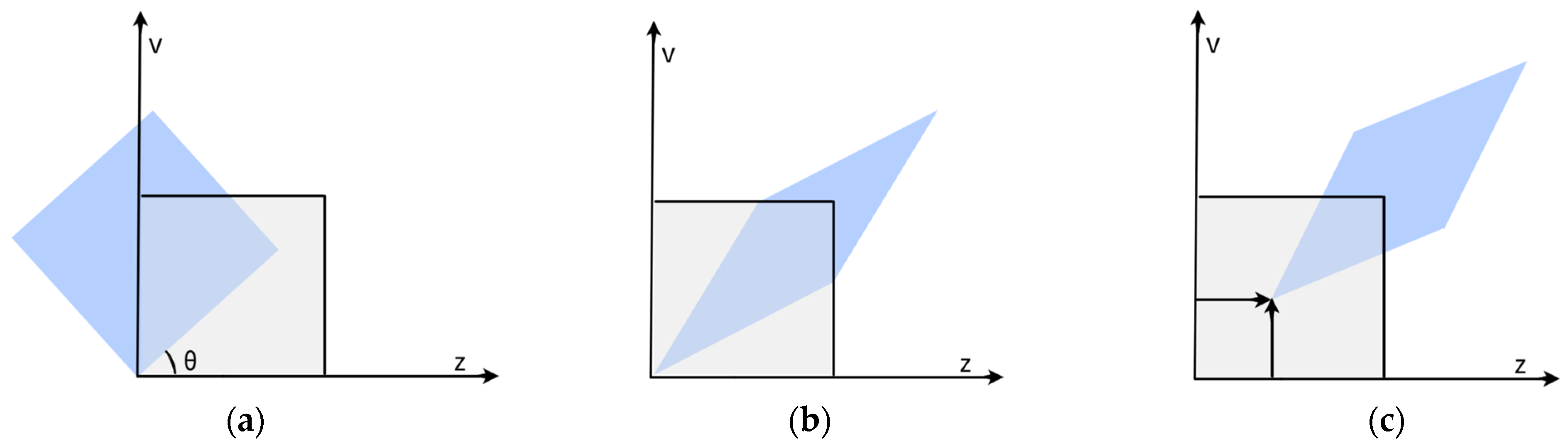
The offset parameter allows the input signal to be shifted in the quaternion domain, which can be useful for signal-processing applications such as image registration and object tracking. Compared to other quaternion-based transformations such as QFT and QLCT, QOLCT has several advantages. First, QOLCT is shift-invariant, meaning that shifting the input signal in the quaternion domain does not change the transform coefficients. This makes QOLCT more robust to noise and distortions in the input signal. Second, QOLCT provides more flexibility in signal-processing applications than QFT or QLCT, because the offset parameter can be used to adjust the phase and position of the input signal. Although QFT and QLCT also have their own unique advantages and applications, QOLCT provides an additional tool for solving a wide range of signal-processing problems. Figure 1 illustrates the role of the offset parameter of QOLCT in comparison with QFT and QLCT.

To obtain left-sided QOLCT, we replace the kernel of OLCT with the QOLCT kernels on the left side of the OLCT definition.

Definition 4.

(left-sided QOLCT). Let $A_n=\left(a_n,b_n,c_n,d_n,{\tau }_n,{\eta }_n\right),$ with the parameters $a_n,b_n,c_n,d_n,{\tau }_n,{\eta }_n\in ℝ,$ such that $a_n{d}_n-b_n{c}_n=1,$ $n=1,2.$ The left-sided QOLCT ${}_L{\mathcal{O}}_{A_1,A_2}^{ℍ,\mu }$ of the 2D quaternion-valued signal $f\in L^2\left({ℝ}^2,ℍ\right)$ is defined by

$${}_L{\mathcal{O}}_{A_1,A_2}^{ℍ,\mu }\left\{f\left(\mathbf{z}\right)\right\}\left(\mathbf{v}\right)={\displaystyle {\int }_{{ℝ}^2}{K}_{A_1}\left(z_1,v_1\right)K_{A_2}\left(z_2,v_2\right)f\left(\mathbf{z}\right)d\mathbf{z},}{b}_1,b_2\ne 0,$$

where $K_{A_n}\left(z_n,v_n\right),$ $n=1,2,$ with $1/\sqrt{\mu }=e^{-\mu \frac{\pi }{4}},$ same as (8).

Lemma 1.

The relationship between left-sided and right-sided QOLCTs is as follows

$${}_L{\mathcal{O}}_{A_1,A_2}^{ℍ,\mu }\left\{f\left(\mathbf{z}\right)\right\}\left(\mathbf{v}\right)=\overline{{}_R{\mathcal{O}}_{A_2,A_1}^{ℍ,-\mu }\left\{\overline{f\left(\mathbf{z}\right)}\right\}\left(\mathbf{v}\right)}.$$

Proof of Lemma 1.

Using the properties of quaternions (2) and (3), the relationship between left-sided QOLCT and right-sided QOLCT is deduced as follows

$$\begin{array}{ll}{}_L{\mathcal{O}}_{A_1,A_2}^{ℍ,\mu }\left\{f\left(\mathbf{z}\right)\right\}\left(\mathbf{v}\right)& ={\displaystyle {\int }_{{ℝ}^2}{K}_{A_1}^{\mu }\left(z_1,v_1\right)K_{A_2}^{\mu }\left(z_2,v_2\right)f\left(\mathbf{z}\right)d\mathbf{z}}\\ & =\overline{{\displaystyle {\int }_{{ℝ}^2}\overline{f\left(\mathbf{z}\right)}{K}_{A_2}^{-\mu }\left(z_2,v_2\right)K_{A_1}^{-\mu }\left(z_1,v_1\right)d\mathbf{z}}}=\overline{{}_R{\mathcal{O}}_{A_2,A_1}^{ℍ,-\mu }\left\{\overline{f\left(\mathbf{z}\right)}\right\}\left(\mathbf{v}\right)}.\end{array}$$

Using Lemma 1, it is easy to perform all the results of right-sided QOLCT to left-sided QOLCT. □

3.2. Relationship with Other Transforms

The relationship between QOLCT and QFT and QLCT of a signal $f$ is described in the next lemmas.

Lemma 2.

The QOLCT of a quaternion-valued signal $f$ with $A_n=\left(a_n,b_n,c_n,d_n,{\tau }_n,{\eta }_n\right),$ $n=1,2,$ can be seen as QFT given by (6) of a signal $f$ in the form

$$\begin{array}{cc}\hfill & {}_R{\mathcal{O}}_{A_1,A_2}^{\mathbb{H},\mu }\left\{f\left(\mathbf{z}\right)\right\}\left(\mathbf{v}\right)\hfill \\ \hfill & ={}_R{\mathcal{F}}^{\mathbb{H}}\left\{f\left(\mathbf{z}\right)e^{\mu \left(a_1/2b_1\right)z_1^2}{e}^{\mu \left(a_2/2b_2\right)z_2^2}{e}^{\mu \left({\tau }_1/b_1\right)z_1}{e}^{\mu \left({\tau }_2/b_2\right)z_2}\right\}\left(\frac{v_1}{b_1},\frac{v_2}{b_2}\right)\hfill \\ \hfill & \times \left(1/\sqrt{2\mu \pi b_1}\right)\left(1/\sqrt{2\mu \pi b_2}\right)e^{-\mu \left(\frac{1}{b_1}{v}_1\left(d_1{\tau }_1-b_1{\eta }_1\right)+\frac{1}{b_2}{v}_2\left(d_2{\tau }_2-b_2{\eta }_2\right)\right)}{e}^{\mu \left(\frac{d_1}{2b_1}\left(v_1^2+{\tau }_1^2\right)+\frac{d_2}{2b_2}\left(v_2^2+{\tau }_2^2\right)\right)}.\hfill \end{array}$$

Proof of Lemma 2.

By a straightforward computation, it follows from the definition of QOLCT that

$$\begin{array}{cc}\hfill & {}_R{\mathcal{O}}_{A_1,A_2}^{\mathbb{H},\mu }\left\{f\left(\mathbf{z}\right)\right\}\left(\mathbf{v}\right)\hfill \\ \hfill & ={\int }_{{\mathbb{R}}^2}\left(f\left(\mathbf{z}\right)e^{\frac{1}{2}\mu \left(\frac{a_1}{b_1}{z}_1^2+\frac{a_2}{b_2}{z}_2^2\right)}{e}^{\mu \left(\frac{{\tau }_1}{b_1}{z}_1+\frac{{\tau }_2}{b_2}{z}_2\right)}\right)e^{-\mu z_1\frac{v_1}{b_1}}{e}^{-\mu z_2\frac{v_2}{b_2}}d\mathbf{z}\hfill \\ \hfill & \times \left(1/\sqrt{2\mu \pi b_1}\right)\left(1/\sqrt{2\mu \pi b_2}\right)e^{-\mu \left(\frac{1}{b_1}{v}_1\left(d_1{\tau }_1-b_1{\eta }_1\right)+\frac{1}{b_2}{v}_2\left(d_2{\tau }_2-b_2{\eta }_2\right)\right)}{e}^{\frac{1}{2}\mu \left(\frac{d_1}{b_1}\left(v_1^2+{\tau }_1^2\right)+\frac{d_2}{b_2}\left(v_2^2+{\tau }_2^2\right)\right)}\hfill \\ \hfill & ={}_R{\mathcal{F}}^{\mathbb{H},\mu }\left\{f\left(\mathbf{z}\right)e^{\frac{1}{2}\mu \left(\frac{a_1}{b_1}{z}_1^2+\frac{a_2}{b_2}{z}_2^2\right)}{e}^{\mu \left(\frac{{\tau }_1}{b_1}{z}_1+\frac{{\tau }_2}{b_2}{z}_2\right)}\right\}\left(\frac{v_1}{b_1},\frac{v_2}{b_2}\right)\hfill \\ \hfill & \times \left(1/\sqrt{2\mu \pi b_1}\right)\left(1/\sqrt{2\mu \pi b_2}\right)e^{-\mu \left(\frac{1}{b_1}{v}_1\left(d_1{\tau }_1-b_1{\eta }_1\right)+\frac{1}{b_2}{v}_2\left(d_2{\tau }_2-b_2{\eta }_2\right)\right)}{e}^{\frac{1}{2}\mu \left(\frac{d_1}{b_1}\left(v_1^2+{\tau }_1^2\right)+\frac{d_2}{b_2}\left(v_2^2+{\tau }_2^2\right)\right)},\hfill \end{array}$$

thus proving the lemma. □

Lemma 3.

The QOLCT of a signal $f$ with $A_n=\left(a_n,b_n,c_n,d_n,{\tau }_n,{\eta }_n\right),$ $n=1,2,$ can be seen as QLCT ${}_R{\mathcal{L}}_{A_1,A_2}^{ℍ}$ of a signal $f$ in the form

$$\begin{array}{ll}{}_R{\mathcal{O}}_{A_1,A_2}^{ℍ,\mu }\left\{f\left(\mathbf{z}\right)\right\}\left(\mathbf{v}\right)=& {}_R{\mathcal{L}}_{A_1,A_2}^{ℍ,\mu }\left\{f\left(\mathbf{z}\right)\right\}\left(\frac{v_1}{b_1},\frac{v_2}{b_2}\right)\frac{1}{\sqrt{2\mu \pi b_1}}\frac{1}{\sqrt{2\mu \pi b_2}}\\ & \times e^{-\mu \left(\frac{1}{b_1}{v}_1\left(d_1{\tau }_1-b_1{\eta }_1\right)+\frac{1}{b_2}{v}_2\left(d_2{\tau }_2-b_2{\eta }_2\right)\right)}{e}^{\mu \left(\frac{d_1}{2b_1}\left(v_1^2+{\tau }_1^2\right)+\frac{d_2}{2b_2}\left(v_2^2+{\tau }_2^2\right)\right)}.\end{array}$$

The proof of the lemma has been omitted due to its resemblance to the proof of the preceding lemma.

3.3. Properties

Below, we introduce the Parseval formula that will be used in proving the uncertainty principle. Next, we give an inversion formula of QOLCT, which is proven in a different way that is more accurate and has fewer computations compared to QLCT. We list the properties of QOLCT in

Table 2. Properties of QOLCT.

Property	QOLCT
Linearity	${}_R{\mathcal{O}}_{A_1,A_2}^{ℍ,\mu }\left\{\alpha f+\beta g\right\}\left(\mathbf{v}\right)=\alpha {}_R{\mathcal{O}}_{A_1,A_2}^{ℍ,\mu }\left\{f\right\}\left(\mathbf{v}\right)+\beta {}_R{\mathcal{O}}_{A_1,A_2}^{ℍ,\mu }\left\{g\right\}\left(\mathbf{v}\right),$ for arbitrary constants $\alpha$ and $\beta .$
Additivity	${}_R{\mathcal{O}}_{A_2}^{\mathbb{H},\mu }\left\{{}_R{\mathcal{O}}_{A_1}^{\mathbb{H},\mu }\left\{f\left(z_1\right)\right\}\left(v_1\right)\right\}\left(v_2\right)={}_R{\mathcal{O}}_{A_1,A_2}^{\mathbb{H},\mu }\left\{f\left(z_1,z_2\right)\right\}\left(v_1,v_2\right),$ where ${}_R{\mathcal{O}}_{A_1}^{ℍ,\mu }$ and ${}_R{\mathcal{O}}_{A_2}^{ℍ,\mu }$ are one-dimensional right-sided QOLCTs.
Translation	$\begin{array}{l}{}_R{\mathcal{O}}_{A_1,A_2}^{ℍ,\mu }\left\{f\left(\mathbf{z}-\mathbf{y}\right)\right\}\left(\mathbf{v}\right)=\exp \left\{\frac{\mu }{2b_1}\left(a_1{y}_1^2-2y_1\left(v_1-{\tau }_1\right)-a_1{y}_1\left(d_1{\tau }_1-b_1{\eta }_1-d_1\left(a_1^2{y}_1^2-2v_1{a}_1{y}_1\right)\right)\right)\right\}\\ \times \exp \left\{\frac{\mu }{2b_2}\left(a_2{y}_2^2-2y_2\left(v_2-{\tau }_2\right)-a_2{y}_2\left(d_2{\tau }_2-b_2{\eta }_2-d_2\left(a_2^2{y}_2^2-2v_2{a}_2{y}_2\right)\right)\right)\right\}{}_R{\mathcal{O}}_{A_1,A_2}^{ℍ,\mu }\left\{f\left(\mathbf{x}\right)\right\}\left(\mathbf{v}-\mathbf{a}\mathbf{y}\right).\end{array}$
Modulation	$\begin{array}{l}{}_R{\mathcal{O}}_{A_1,A_2}^{ℍ,\mu }\left\{f(\mathbf{z})e^{\mu \left(z_1{w}_1+z_2{w}_2\right)}\right\}(\mathbf{v})\\ =\exp \left\{-\mu \left(w_1+\frac{d_1{b}_1{w}_1^2}{2}-d_1{v}_1{w}_1+w_2+\frac{d_2{b}_2{w}_2^2}{2}-d_2{v}_2{w}_2\right)\right\}{·}_R{\mathcal{O}}_{A_1,A_2}^{ℍ,\mu }\left\{f(\mathbf{z})\right\}(\mathbf{v}-\mathbf{b}\mathbf{w}).\end{array}$
Parity	${}_R{\mathcal{O}}_{A_1,A_2}^{ℍ,\mu }\left\{Pf(\mathbf{z})\right\}(\mathbf{v}{)=}_R{\mathcal{O}}_{A_1^{\prime },A_2^{\prime }}^{ℍ,\mu }\left\{f(\mathbf{y})\right\}(-\mathbf{v}),$ where $A_n^{\prime }=\left(a_n, b_n, c_n, d_n, -{\tau }_n, -{\eta }_n\right),$ $n=1,2.$ $Pf(\mathbf{z})$ is the parity of $f(\mathbf{z}),$ that is given by $Pf(\mathbf{z})=f(-\mathbf{z}).$
Parseval formula	${〈{}_R{\mathcal{O}}_{A_1,A_2}^{ℍ,\mu }\left\{f\right\},{ }_R{\mathcal{O}}_{A_1,A_2}^{ℍ,\mu }\left\{g\right\}〉}_{L^2({ℝ}^2,ℍ)}={〈f, g〉}_{L^2({ℝ}^2,ℍ)}.$
Inversion formula	$f(\mathbf{z})={\displaystyle {\int }_{{ℝ}^2}}{ }_R{\mathcal{O}}_{A_1,A_2}^{ℍ,\mu }\left\{f\right\}(\mathbf{v}( \overline{K_{A_2}(z_2,v_2)} \overline{K_{A_1}(z_1,v_1)}d\mathbf{v}.$

.

Property 1.

(Parseval formula). Let ${}_R{\mathcal{O}}_{A_1,A_2}^{ℍ,\mu }\left\{f\right\}$ and ${}_R{\mathcal{O}}_{A_1,A_2}^{ℍ,\mu }\left\{g\right\}$ be right-sided QOLCT of quaternion-valued functions $f$ and $g,$ respectively. Then

$${〈{}_R{\mathcal{O}}_{A_1,A_2}^{ℍ,\mu }\left\{f\right\},{ }_R{\mathcal{O}}_{A_1,A_2}^{ℍ,\mu }\left\{g\right\}〉}_{L^2({ℝ}^2,ℍ)}={〈f, g〉}_{L^2({ℝ}^2,ℍ)}.$$

Proof of Property 1.

By Equation (4) and the inner product of any two quaternions, we have

$$\begin{array}{cc}\hfill & {〈{}_R{\mathcal{O}}_{A_1,A_2}^{\mathbb{H},\mu }\left\{f\right\},{}_R{\mathcal{O}}_{A_1,A_2}^{\mathbb{H},\mu }\left\{g\right\}〉}_{L^2({\mathbb{R}}^2,\mathbb{H})}\hfill \\ \hfill & ={\int }_{{\mathbb{R}}^2}{}_R{\mathcal{O}}_{A_1,A_2}^{\mathbb{H},\mu }\left\{f\right\}\left(\mathbf{v}\right)\overline{{}_R{\mathcal{O}}_{A_1,A_2}^{\mathbb{H},\mu }\left\{g\right\}\left(\mathbf{v}\right)}d\mathbf{v}\hfill \\ \hfill & ={\int }_{{\mathbb{R}}^2}\left({\int }_{{\mathbb{R}}^2}f\left(\mathbf{z}\right)K_{A_1}(z_1,v_1)K_{A_2}(z_2,v_2)d\mathbf{z}\right)\overline{\left({\int }_{{\mathbb{R}}^2}g\left(\mathbf{x}\right)K_{A_1}(x_1,v_1)K_{A_2}(x_2,v_2)d\mathbf{x}\right)}d\mathbf{v}\hfill \\ \hfill & ={\int }_{{\mathbb{R}}^2}{\int }_{{\mathbb{R}}^2}{\int }_{{\mathbb{R}}^2}f\left(\mathbf{z}\right)K_{A_1}(z_1,v_1)K_{A_2}(z_2,v_2)\overline{K_{A_2}(x_2,v_2)}\overline{K_{A_1}(x_1,v_1)}\overline{g\left(\mathbf{x}\right)}d\mathbf{z}d\mathbf{x}d\mathbf{v}\hfill \\ \hfill & ={\int }_{{\mathbb{R}}^6}f(z_1,z_2)K_{A_1}(z_1,v_1)\left(\frac{1}{2\pi \sqrt{{\mu }^2{b}_1{b}_2}}exp\left\{\frac{\mu }{2b_2}\left(a_2(z_2^2-x_2^2)+2{\tau }_2(z_2-x_2)\right)\right\}\right)\hfill \\ \hfill & \times exp\left\{\frac{-\mu v_2(z_2-x_2)}{b_2}\right\}\overline{K_{A_1}(x_1,v_1)} \overline{g(x_1,x_2)}d{z}_{1}d{z}_{2}d{x}_{1}d{x}_{2}d{v}_{1}d{v}_2\hfill \\ \hfill & ={\int }_{{\mathbb{R}}^5}f(z_1,z_2)K_{A_1}(z_1,v_1)\frac{1}{\sqrt{{\mu }^2{b}_1{b}_2}}exp\left\{\frac{\mu }{2b_2}\left(a_2(z_2^2-x_2^2)+2{\tau }_2(z_2-x_2)\right)\right\}\hfill \\ \hfill & \times \left(\frac{1}{2\pi }{\int }_{\mathbb{R}}exp\left\{\frac{-\mu v_2(z_2-x_2)}{b_2}\right\}d{v}_2\right)\overline{K_{A_1}(x_1,v_1)} \overline{g(x_1,x_2)}d{z}_{1}d{z}_{2}d{x}_{1}d{x}_{2}d{v}_1\hfill \\ \hfill & ={\int }_{{\mathbb{R}}^5}f(z_1,z_2)K_{A_1}(z_1,v_1)\frac{1}{\sqrt{{\mu }^2{b}_1{b}_2}}exp\left\{\frac{\mu }{2b_2}\left(a_2(z_2^2-x_2^2)+2{\tau }_2(z_2-x_2)\right)\right\}\hfill \\ \hfill & \times \left(b_2\delta (z_2-x_2)\right)\overline{K_{A_1}(x_1,v_1)} \overline{g(x_1,x_2)}d{z}_{1}d{z}_{2}d{x}_{1}d{x}_{2}d{v}_1\hfill \\ \hfill & ={\int }_{{\mathbb{R}}^4}f(z_1,z_2)K_{A_1}(z_1,v_1)\frac{b_2}{\sqrt{{\mu }^2{b}_1{b}_2}}\overline{K_{A_1}(x_1,v_1)} \overline{g(x_1,z_2)}d{z}_{1}d{z}_{2}d{x}_{1}d{v}_1\hfill \\ \hfill & ={\int }_{{\mathbb{R}}^4}f(z_1,z_2)\frac{1}{\sqrt{\mu 2\pi b_1}}exp\left\{\frac{\mu }{2b_1}\left(a_1{z}_1^2-2z_1\left(v_1-{\tau }_1\right)-2v_1\left(d_1{\tau }_1-b_1{\eta }_1\right)+d_1\left(v_1^2+{\tau }_1^2\right)\right)\right\}\frac{b_2}{\sqrt{{\mu }^2{b}_1{b}_2}}\hfill \\ \hfill & \times \overline{\frac{1}{\sqrt{\mu 2\pi b_1}}exp\left\{\frac{\mu }{2b_1}\left(a_1{x}_1^2-2x_1\left(v_1-{\tau }_1\right)-2v_1\left(d_1{\tau }_1-b_1{\eta }_1\right)+d_1\left(v_1^2+{\tau }_1^2\right)\right)\right\}}\overline{g(x_1,z_2)}d{z}_{1}d{z}_{2}d{x}_{1}d{v}_1\hfill \\ \hfill & ={\int }_{{\mathbb{R}}^3}f(z_1,z_2)\frac{1}{\sqrt{{\mu }^2{b}_1{b}_2}}exp\left\{\frac{\mu }{2b_1}\left(a_1(z_1^2-x_1^2)+2{\tau }_1(z_1-x_1)\right)\right\}\frac{1}{2\pi }\hfill \\ \hfill & \times {\int }_{\mathbb{R}}exp\left\{\frac{\mu }{2b_1}{v}_1(z_1-x_1)\right\}d{v}_1\overline{g(x_1,z_2)}d{z}_{1}d{z}_{2}d{x}_1\hfill \\ \hfill & ={\int }_{{\mathbb{R}}^3}f(z_1,z_2)\frac{1}{\sqrt{{\mu }^2{b}_1{b}_2}}\frac{b_2}{\sqrt{{\mu }^2{b}_1{b}_2}}exp\left\{\frac{\mu }{2b_1}\left(a_1(z_1^2-x_1^2)+2{\tau }_1(z_1-x_1)\right)\right\}\hfill \\ \hfill & \times \left(b_1\delta (z_1-x_1)\right)\overline{g(x_1,z_2)}d{z}_{1}d{z}_{2}d{x}_1\hfill \\ \hfill & ={\int }_{{\mathbb{R}}^2}f(z_1,z_2)\frac{1}{\sqrt{{\mu }^2{b}_1{b}_2}}\frac{b_1{b}_2}{\sqrt{{\mu }^2{b}_1{b}_2}}\overline{g(z_1,z_2)}d{z}_{1}d{z}_2\hfill \\ \hfill & ={\int }_{{\mathbb{R}}^2}f(z_1,z_2)\overline{g(z_1,z_2)}d{z}_{1}d{z}_2\hfill \\ \hfill & ={〈f,g〉}_{L^2({\mathbb{R}}^2,\mathbb{H})}.\square \hfill \end{array}$$

Property 2.

(Inversion formula). For an arbitrary quaternion-valued function $g\in L^2({ℝ}^2,ℍ)$, using the Parseval formula (Property 1) and Fubini’s theorem, we have

$$\begin{array}{ll}{〈f,g〉}_{L^2({\mathbb{R}}^2,\mathbb{H})}& ={〈{}_R{\mathcal{O}}_{A_1,A_2}^{\mathbb{H},\mu }\left\{f\right\},{}_R{\mathcal{O}}_{A_1,A_2}^{\mathbb{H},\mu }\left\{g\right\}〉}_{L^2({\mathbb{R}}^2,\mathbb{H})}\\ & ={\int }_{{\mathbb{R}}^2} {}_R{\mathcal{O}}_{A_1,A_2}^{\mathbb{H},\mu }\left\{f\right\}\left(\mathbf{v}\right)\overline{\left({\int }_{{\mathbb{R}}^2}g\left(\mathbf{z}\right)K_{A_1}(z_1,v_1)K_{A_2}(z_2,v_2)d\mathbf{z}\right)}d\mathbf{v}\\ & ={\int }_{{\mathbb{R}}^2}{\int }_{{\mathbb{R}}^2} {}_R{\mathcal{O}}_{A_1,A_2}^{\mathbb{H},\mu }\left\{f\right\}\left(\mathbf{v}\right)\overline{K_{A_2}(z_2,v_2)} \overline{K_{A_1}(z_1,v_1)} \overline{g\left(\mathbf{z}\right)}d\mathbf{z}d\mathbf{v}\\ & ={\int }_{{\mathbb{R}}^2}\left({\int }_{{\mathbb{R}}^2} {}_R{\mathcal{O}}_{A_1,A_2}^{\mathbb{H},\mu }\left\{f\right\}\left(\mathbf{v}\right)\overline{K_{A_2}(z_2,v_2)} \overline{K_{A_1}(z_1,v_1)}d\mathbf{v}\right)\overline{g\left(\mathbf{z}\right)}d\mathbf{z}\hfill \\ & ={〈{\int }_{{\mathbb{R}}^2} {}_R{\mathcal{O}}_{A_1,A_2}^{\mathbb{H},\mu }\left\{f\right\}\left(\mathbf{v}\right)\overline{K_{A_2}(z_2,v_2)} \overline{K_{A_1}(z_1,v_1)}d\mathbf{v},g〉}_{L^2({\mathbb{R}}^2,\mathbb{H})}\end{array}$$

Equivalently, we have

$$f(\mathbf{z})={\displaystyle {\int }_{{ℝ}^2}}{ }_R{\mathcal{O}}_{A_1,A_2}^{ℍ,\mu }\left\{f\right\}(\mathbf{v}) \overline{K_{A_2}(z_2,v_2)} \overline{K_{A_1}(z_1,v_1)}d\mathbf{v}, a.e. \square$$

4. Convolution and Correlation Theorems for QOLCT

Convolution is an operation used in many fields, such as communications, computer vision, signal and image processing, radar systems, also used in finding statistical relationships, etc. Correlation is another important operation with applications in astronomy, engineering, financial analysis, and statistical physics. Because of their simplicity, it is easy to implement and can be computed very efficiently. It is necessary to study QOLCT convolution and correlation properties to strengthen its applications. For this reason, we present the next two subsections.

4.1. Convolution Theorem for QOLCT

In this subsection, we define the convolution of the 2D right-sided QOLCT.

Definition 5.

For $f,g\in L^2\left({ℝ}^2,ℍ\right),$ the convolution operator of QOLCT is defined by

$$\left(f{\otimes }^{A_1,A_2} g\right)\left(\mathbf{z}\right)={\displaystyle {\int }_{{ℝ}^2}f\left(\mathbf{t}\right)g\left(\mathbf{z}-\mathbf{t}\right)e^{\mu \left(a_1/b_1\right)t_1\left(t_1-z_1\right)}}{e}^{\mu \left(a_2/b_2\right)t_2\left(t_2-z_2\right)}d\mathbf{t}.$$

(9)

Definition 5 implies the subsequent theorem, which shows how two quaternion-valued functions’ convolution interacts with their QOLCTs.

Theorem 1.

Let

$$\begin{array}{l}f\left(\mathbf{z}\right)=f_0\left(\mathbf{z}\right)+i f_1\left(\mathbf{z}\right)+j f_2\left(\mathbf{z}\right)+k f_3\left(\mathbf{z}\right),\\ g\left(\mathbf{z}\right)=g_0\left(\mathbf{z}\right)+i{ \mathrm{g}}_1\left(\mathbf{z}\right)+j{ \mathrm{g}}_2\left(\mathbf{z}\right)+k{ \mathrm{g}}_3\left(\mathbf{z}\right),\end{array}$$

(10)

belong to $L^2\left({ℝ}^2,ℍ\right)$. Then, the QOLCT of the convolution of $f$ and $g$ is given by

$$\begin{array}{ll}{}_R{\mathcal{O}}_{A_1,A_2}^{\mathbb{H},\mu }\left\{f{\otimes }^{A_1,A_2} g\right\}\left(\mathbf{v}\right)=& \left({}_R{\mathcal{O}}_{A_1,A_2}^{\mathbb{H},\mu }\left\{g\right\}\left(\mathbf{v}\right){}_R{\mathcal{O}}_{A_1,A_2}^{\mathbb{H},\mu }\left\{f_0\right\}\left(\mathbf{v}\right)\right.\\ & +i {}_R{\mathcal{O}}_{A_1,A_2}^{\mathbb{H},\mu }\left\{g\right\}\left(\mathbf{v}\right){}_R{\mathcal{O}}_{A_1,A_2}^{\mathbb{H},\mu }\left\{f_1\right\}\left(\mathbf{v}\right)\hfill \\ & +j {}_R{\mathcal{O}}_{A_1,A_2}^{\mathbb{H},\mu }\left\{g\right\}\left(\mathbf{v}\right){}_R{\mathcal{O}}_{A_1,A_2}^{\mathbb{H},\mu }\left\{f_2\right\}\left(\mathbf{v}\right)\hfill \\ & \left.+k {}_R{\mathcal{O}}_{A_1,A_2}^{\mathbb{H},\mu }\left\{g\right\}\left(\mathbf{v}\right){}_R{\mathcal{O}}_{A_1,A_2}^{\mathbb{H},\mu }\left\{f_3\right\}\left(\mathbf{v}\right)\right)\hfill \\ & \times \sqrt{2\pi b_1\mu }\sqrt{2\pi b_2\mu }{e}^{\mu \left(\left(v_1/b_1\right)\left(d_1{\tau }_1-b_1{\eta }_1\right)-\left(d_1/2b_1\right)\left(v_1^2+{\tau }_1^2\right)\right)}{e}^{\mu \left(\left(v_2/b_2\right)\left(d_2{\tau }_2-b_2{\eta }_2\right)-\left(d_2/2b_2\right)\left(v_2^2+{\tau }_2^2\right)\right)}.\hfill \end{array}$$

Proof of Theorem 1.

Let ${}_R{\mathcal{O}}_{A_1,A_2}^{ℍ,\mu }\left\{f\right\}$ and ${}_R{\mathcal{O}}_{A_1,A_2}^{ℍ,\mu }\left\{g\right\}$ denote QOLCTs of $f$ and $g,$ respectively. Expanding QOLCT of the left-hand side of the above identity using (9), we obtain

$$\begin{array}{l}{}_R{\mathcal{O}}_{A_1,A_2}^{ℍ,\mu }\left\{f{\otimes }^{A_1,A_2} g\right\}\left(\mathbf{v}\right)\\ ={\displaystyle {\int }_{{ℝ}^2}\left(f{\otimes }^{A_1,A_2} g\right)\left(\mathbf{z}\right)}{K}_{A_1}\left(z_1,v_1\right)K_{A_2} \left(z_2,v_2\right)d\mathbf{z}\\ ={\displaystyle {\int }_{{ℝ}^2}\left[{\displaystyle {\int }_{{ℝ}^2}f\left(\mathbf{t}\right)g\left(\mathbf{z}-\mathbf{t}\right)e^{\mu \left(a_1/b_1\right)t_1\left(t_1-z_1\right)}}{e}^{\mu \left(a_2/b_2\right)t_2\left(t_2-z_2\right)}d\mathbf{t}\right]}{K}_{A_1}\left(z_1,v_1\right) K_{A_2}\left(z_2,v_2\right)d\mathbf{z}.\end{array}$$

By changing variables $\mathbf{z}-\mathbf{t}=\mathbf{y}$ in the above expression, we have

$$\begin{array}{ll}{}_R{\mathcal{O}}_{A_1,A_2}^{\mathbb{H},\mu }\left\{f{\otimes }^{A_1,A_2} g\right\}\left(\mathbf{v}\right)=\hfill & {\int }_{{\mathbb{R}}^2}\left[{\int }_{{\mathbb{R}}^2}f\left(\mathbf{t}\right)g\left(\mathbf{y}\right)e^{\mu \left(a_1/b_1\right)\left(-t_1{y}_1\right)}{e}^{\mu \left(a_2/b_2\right)\left(-t_2{y}_2\right)}d\mathbf{t}\right]\frac{1}{\sqrt{2\mu \pi b_1}}\frac{1}{\sqrt{2\mu \pi b_2}}\\ & \times e^{\mu \left(\left(a_1/2b_1\right){\left(y_1+t_1\right)}^2-\left(1/b_1\right)\left(y_1+t_1\right)\left(v_1-{\tau }_1\right)-\left(1/b_1\right)v_1\left(d_1{\tau }_1-b_1{\eta }_1\right)+\left(d_1/2b_1\right)\left(v_1^2+{\tau }_1^2\right)\right)}\hfill \\ & \times e^{\mu \left(\left(a_2/2b_2\right){\left(y_2+t_2\right)}^2-\left(1/b_2\right)\left(y_2+t_2\right)\left(v_2-{\tau }_2\right)-\left(1/b_2\right)v_2\left(d_2{\tau }_2-b_2{\eta }_2\right)+\left(d_2/2b_2\right)\left(v_2^2+{\tau }_2^2\right)\right)}d\mathbf{y}\hfill \\ \hfill =& {\int }_{{\mathbb{R}}^2}{\int }_{{\mathbb{R}}^2}f\left(\mathbf{t}\right)g\left(\mathbf{y}\right)\frac{1}{\sqrt{2\mu \pi b_1}}\frac{1}{\sqrt{2\mu \pi b_2}}\hfill \\ & \times e^{\mu \left(\left(a_1/2b_1\right)y_1^2-\left(1/b_1\right)\left(v_1-{\tau }_1\right)y_1-\left(v_1/b_1\right)\left(d_1{\tau }_1-b_1{\eta }_1\right)+\left(d_1/2b_1\right)\left(v_1^2+{\tau }_1^2\right)\right)}\hfill \\ & \times e^{\mu \left(\left(a_2/2b_2\right)y_2^2-\left(1/b_1\right)\left(v_2-{\tau }_2\right)y_2-\left(v_2/b_2\right)\left(d_2{\tau }_2-b_2{\eta }_2\right)+\left(d_2/2b_2\right)\left(v_2^2+{\tau }_2^2\right)\right)}\hfill \\ & \times e^{\mu \left(a_1/2b_1\right)t_1^2}{e}^{-\mu \left(1/b_1\right)\left(v_1-{\tau }_1\right)t_1}{e}^{\mu \left(a_2/2b_2\right)t_2^2}{e}^{-\mu \left(1/b_2\right)\left(v_2-{\tau }_2\right)t_2}d\mathbf{y}d\mathbf{t}.\hfill \end{array}$$

Applying the QOLCT Definition (7) yields

$$\begin{array}{l}{}_R{\mathcal{O}}_{A_1,A_2}^{ℍ,\mu }\left\{f{\otimes }^{A_1,A_2} g\right\}\left(\mathbf{v}\right)\\ ={\displaystyle {\int }_{{ℝ}^2}f\left(\mathbf{t}\right) {}_R{\mathcal{O}}_{A_1,A_2}^{ℍ,\mu }\left\{g\right\}\left(\mathbf{v}\right)e^{\mu \left(a_1/2b_1\right)t_1^2}{e}^{-\mu \left(1/b_1\right)\left(v_1-{\tau }_1\right)t_1}{e}^{\mu \left(a_2/2b_2\right)t_2^2}{e}^{-\mu \left(1/b_2\right)\left(v_2-{\tau }_2\right)t_2}d\mathbf{t}}.\end{array}$$

Now we decompose $f\left(\mathbf{t}\right)$ into $f_0\left(\mathbf{t}\right)+i f_1\left(\mathbf{t}\right)+j f_2\left(\mathbf{t}\right)+k f_3\left(\mathbf{t}\right).$ This gives

$$\begin{array}{ll}\hfill {}_R{\mathcal{O}}_{A_1,A_2}^{\mathbb{H},\mu }\left\{f{\otimes }^{A_1,A_2} g\right\}\left(\mathbf{v}\right)=& {\int }_{{\mathbb{R}}^2}\left[f_0\left(\mathbf{t}\right)+i f_1\left(\mathbf{t}\right)+j f_2\left(\mathbf{t}\right)+k f_3\left(\mathbf{t}\right)\right]{}_R{\mathcal{O}}_{A_1,A_2}^{\mathbb{H},\mu }\left\{g\right\}\left(\mathbf{v}\right)\\ & \times e^{\mu \left(a_1/2b_1\right)t_1^2}{e}^{-\mu \left(1/b_1\right)\left(v_1-{\tau }_1\right)t_1}{e}^{\mu \left(a_2/2b_2\right)t_2^2}{e}^{-\mu \left(1/b_2\right)\left(v_2-{\tau }_2\right)t_2}d\mathbf{t}\hfill \\ \hfill =& {\int }_{{\mathbb{R}}^2}\left[{}_R{\mathcal{O}}_{A_1,A_2}^{\mathbb{H},\mu }\left\{g\right\}\left(\mathbf{v}\right)f_0\left(\mathbf{t}\right)+i {}_R{\mathcal{O}}_{A_1,A_2}^{\mathbb{H},\mu }\left\{g\right\}\left(\mathbf{v}\right)f_1\left(\mathbf{t}\right)+j {}_R{\mathcal{O}}_{A_1,A_2}^{\mathbb{H},\mu }\left\{g\right\}\left(\mathbf{v}\right)f_2\left(\mathbf{t}\right)+k {}_R{\mathcal{O}}_{A_1,A_2}^{\mathbb{H},\mu }\left\{g\right\}\left(\mathbf{v}\right)f_3\left(\mathbf{t}\right)\right]\hfill \\ & \times e^{\mu \left(a_1/2b_1\right)t_1^2}{e}^{-\mu \left(1/b_1\right)\left(v_1-{\tau }_1\right)t_1}{e}^{\mu \left(a_2/2b_2\right)t_2^2}{e}^{-\mu \left(1/b_2\right)\left(v_2-{\tau }_2\right)t_2}d\mathbf{t}.\hfill \end{array}$$

Post-multiplying both sides of the above identity by $\left(1/\sqrt{2\pi \mu b_1}\right)e^{\mu \left(-\left(v_1/b_1\right)\left(d_1{\tau }_1-b_1{\eta }_1\right)+\left(d_1/2b_1\right)\left(v_1^2+{\tau }_1^2\right)\right)}$ and $\left(1/\sqrt{2\pi \mu b_2}\right)e^{\mu \left(-\left(v_2/b_2\right)\left(d_2{\tau }_2-b_2{\eta }_2\right)+\left(d_2/2b_2\right)\left(v_2^2+{\tau }_2^2\right)\right)},$ we obtain

$$\begin{array}{cc}\hfill & {}_R{\mathcal{O}}_{A_1,A_2}^{\mathbb{H},\mu }\left\{f{\otimes }^{A_1,A_2} g\right\}\left(\mathbf{v}\right)\hfill \\ \hfill & \times \frac{1}{\sqrt{2\pi \mu b_1}}{e}^{\mu \left(-\left(v_1/b_1\right)\left(d_1{\tau }_1-b_1{\eta }_1\right)+\left(d_1/2b_1\right)\left(v_1^2+{\tau }_1^2\right)\right)}\frac{1}{\sqrt{2\pi \mu b_2}}{e}^{\mu \left(-\left(v_2/b_2\right)\left(d_2{\tau }_2-b_2{\eta }_2\right)+\left(d_2/2b_2\right)\left(v_2^2+{\tau }_2^2\right)\right)}\hfill \\ \hfill & ={\int }_{{\mathbb{R}}^2}\left[{}_R{\mathcal{O}}_{A_1,A_2}^{\mathbb{H},\mu }\left\{g\right\}\left(\mathbf{v}\right)f_0\left(\mathbf{t}\right)+i {}_R{\mathcal{O}}_{A_1,A_2}^{\mathbb{H},\mu }\left\{g\right\}\left(\mathbf{v}\right)f_1\left(\mathbf{t}\right)+j {}_R{\mathcal{O}}_{A_1,A_2}^{\mathbb{H},\mu }\left\{g\right\}\left(\mathbf{v}\right)f_2\left(\mathbf{t}\right)+k {}_R{\mathcal{O}}_{A_1,A_2}^{\mathbb{H},\mu }\left\{g\right\}\left(\mathbf{v}\right)f_3\left(\mathbf{t}\right)\right]\hfill \\ \hfill & \times \frac{1}{\sqrt{2\pi \mu b_1}}{e}^{\mu \left(\left(a_1/2b_1\right)t_1^2-\left(1/b_1\right)\left(v_1-{\tau }_1\right)t_1-\left(v_1/b_1\right)\left(d_1{\tau }_1-b_1{\eta }_1\right)+\left(d_1/2b_1\right)\left(v_1^2+{\tau }_1^2\right)\right)}\frac{1}{\sqrt{2\pi \mu b_2}}{e}^{\mu \left(\left(a_2/2b_2\right)t_2^2-\left(1/b_1\right)\left(v_2-{\tau }_2\right)t_2-\left(v_2/b_2\right)\left(d_2{\tau }_2-b_2{\eta }_2\right)+\left(d_2/2b_2\right)\left(v_2^2+{\tau }_2^2\right)\right)}d\mathbf{t}.\hfill \end{array}$$

Finally, arrive at

$$\begin{array}{cc}\hfill & {}_R{\mathcal{O}}_{A_1,A_2}^{\mathbb{H},\mu }\left\{f{\otimes }^{A_1,A_2} g\right\}\left(\mathbf{v}\right)\hfill \\ \hfill & \times \frac{1}{\sqrt{2\pi \mu b_1}}{e}^{\mu \left(-\left(v_1/b_1\right)\left(d_1{\tau }_1-b_1{\eta }_1\right)+\left(d_1/2b_1\right)\left(v_1^2+{\tau }_1^2\right)\right)}\frac{1}{\sqrt{2\pi \mu b_2}}{e}^{\mu \left(-\left(v_2/b_2\right)\left(d_2{\tau }_2-b_2{\eta }_2\right)+\left(d_2/2b_2\right)\left(v_2^2+{\tau }_2^2\right)\right)}\hfill \\ \hfill & =\left({}_R{\mathcal{O}}_{A_1,A_2}^{\mathbb{H},\mu }\left\{g\right\}\left(\mathbf{v}\right){}_R{\mathcal{O}}_{A_1,A_2}^{\mathbb{H},\mu }\left\{f_0\right\}\left(\mathbf{v}\right)+i {}_R{\mathcal{O}}_{A_1,A_2}^{\mathbb{H},\mu }\left\{g\right\}\left(\mathbf{v}\right){}_R{\mathcal{O}}_{A_1,A_2}^{\mathbb{H},\mu }\left\{f_1\right\}\left(\mathbf{v}\right)\right.\hfill \\ \hfill & \left.+j {}_R{\mathcal{O}}_{A_1,A_2}^{\mathbb{H},\mu }\left\{g\right\}\left(\mathbf{v}\right){}_R{\mathcal{O}}_{A_1,A_2}^{\mathbb{H},\mu }\left\{f_2\right\}\left(\mathbf{v}\right)+k {}_R{\mathcal{O}}_{A_1,A_2}^{\mathbb{H},\mu }\left\{g\right\}\left(\mathbf{v}\right){}_R{\mathcal{O}}_{A_1,A_2}^{\mathbb{H},\mu }\left\{f_3\right\}\left(\mathbf{v}\right)\right),\hfill \end{array}$$

which completes the proof. □

Property 3.

(Linearity). For quaternion-valued functions $f, g$ and $h,$ and quaternion constants $\alpha$ and $\beta$ we have

$$\left[\left(\alpha f+\beta g\right){\otimes }^{A_1,A_2} h\right]\left(\mathbf{z}\right)=\alpha \left[f{\otimes }^{A_1,A_2} h\right]\left(\mathbf{z}\right)+\beta \left[g{\otimes }^{A_1,A_2} h\right]\left(\mathbf{z}\right).$$

Property 4.

(Distributive).For quaternion-valued functions $f, g$ and $h,$ we have

$$\left[h{\otimes }^{A_1,A_2} \left(f+g\right)\right]\left(\mathbf{z}\right)=\left[h{\otimes }^{A_1,A_2} f\right]\left(\mathbf{z}\right)+\left[h{\otimes }^{A_1,A_2} g\right]\left(\mathbf{z}\right).$$

The convolution theorem has important practical significance for QOLCT, as it allows for the efficient computation of QOLCT using Fourier-based techniques. The convolution theorem allows for the point-wise multiplication of the transformed input signal and the transformed kernel function, reducing the computation to a single inverse QOLCT. The kernel function enables the shift-invariance and flexibility of QOLCT, making QOLCT more practical and accessible for a wide range of signal-processing applications such as filtering, cross-correlation, and feature extraction.

4.2. Correlation Theorem for QOLCT

In this subsection, we define the correlation of the 2D right-sided QOLCT.

Definition 6.

For $f,g\in L^2\left({ℝ}^2,ℍ\right),$ the correlation operator of QOLCT is defined as

$$\left(f{\circ }^{A_1,A_2} g\right)\left(\mathbf{z}\right)={\displaystyle {\int }_{{ℝ}^2}\overline{f\left(\mathbf{t}\right)}g\left(\mathbf{t}+\mathbf{z}\right)e^{\mu \left(a_1/b_1\right)t_1\left(t_1+z_1\right)}}{e}^{\mu \left(a_2/b_2\right)t_2\left(t_2+z_2\right)}d\mathbf{t}.$$

(11)

Then, we reap a consequence of Definition 6.

Theorem 2.

Suppose that$f,g\in L^2\left({ℝ}^2,ℍ\right),$ QOLCT of the correlation of $f$ and $g$ is given by

$$\begin{array}{ll}{}_R{\mathcal{O}}_{A_1,A_2}^{ℍ,\mu }\left\{f{\circ }^{A_1,A_2} g\right\}\left(\mathbf{v}\right)=& \left({}_R{\mathcal{O}}_{A_1,A_2}^{ℍ,\mu }\left\{g\right\}\left(\mathbf{v}\right){}_R{\mathcal{O}}_{A_1,A_2}^{ℍ,\mu }\left\{f_0\right\}\left(\mathbf{v}\right)\right.\\ & -i {}_R{\mathcal{O}}_{A_1,A_2}^{ℍ,\mu }\left\{g\right\}\left(\mathbf{v}\right){}_R{\mathcal{O}}_{A_1,A_2}^{ℍ,\mu }\left\{f_1\right\}\left(-\mathbf{v}\right)\\ & -j {}_R{\mathcal{O}}_{A_1,A_2}^{ℍ,\mu }\left\{g\right\}\left(\mathbf{v}\right){}_R{\mathcal{O}}_{A_1,A_2}^{ℍ,\mu }\left\{f_2\right\}\left(-\mathbf{v}\right)\\ & \left.-k {}_R{\mathcal{O}}_{A_1,A_2}^{ℍ,\mu }\left\{g\right\}\left(\mathbf{v}\right){}_R{\mathcal{O}}_{A_1,A_2}^{ℍ,\mu }\left\{f_3\right\}\left(-\mathbf{v}\right)\right).\end{array}$$

When $A_n=(a_n,b_n,c_n,d_n,0,0),$ $n=1,2$ the above expression reduces to the correlation of right-sided QLCT ${}_R{\mathcal{L}}_{A_1,A_2}^{ℍ,\mu }\left\{f{\circ }^{A_1,A_2} g\right\}\left(\mathbf{v}\right)$ as

$$\begin{array}{ll}{}_R{\mathcal{L}}_{A_1,A_2}^{ℍ,\mu }\left\{f{\circ }^{A_1,A_2} g\right\}\left(\mathbf{v}\right)=& \left({}_R{\mathcal{L}}_{A_1,A_2}^{ℍ,\mu }\left\{g\right\}\left(\mathbf{v}\right){}_R{\mathcal{L}}_{A_1,A_2}^{ℍ,\mu }\left\{f_0\right\}\left(\mathbf{v}\right)\right.\\ & -i {}_R{\mathcal{L}}_{A_1,A_2}^{ℍ,\mu }\left\{g\right\}\left(\mathbf{v}\right){}_R{\mathcal{L}}_{A_1,A_2}^{ℍ,\mu }\left\{f_1\right\}\left(-\mathbf{v}\right)\\ & -j {}_R{\mathcal{L}}_{A_1,A_2}^{ℍ,\mu }\left\{g\right\}\left(\mathbf{v}\right){}_R{\mathcal{L}}_{A_1,A_2}^{ℍ,\mu }\left\{f_2\right\}\left(-\mathbf{v}\right)\\ & \left.-k {}_R{\mathcal{L}}_{A_1,A_2}^{ℍ,\mu }\left\{g\right\}\left(\mathbf{v}\right){}_R{\mathcal{L}}_{A_1,A_2}^{ℍ,\mu }\left\{f_3\right\}\left(-\mathbf{v}\right)\right).\end{array}$$

When $A_1=A_2=(0,1,-1,0,0,0),$ the convolution of right-sided QFT is recovered as follows

$${}_R{\mathcal{F}}^{ℍ,\mu }\left\{f{\circ }^{A_1,A_2} g\right\}\left(\mathbf{v}\right)={}_R\mathcal{F}{}^{ℍ,\mu }\left\{g\right\}\left(\mathbf{v}\right){}_R\mathcal{F}{}^{ℍ,\mu }\left\{\overline{f}\right\}\left(-\mathbf{v}\right)\sqrt{2\pi \mu b_1}\sqrt{2\pi \mu b_2.}$$

Proof of Theorem 2.

From the QOLCT Definition (7) and correlation Definition (11), we obtain

$$\begin{array}{cc}\hfill & {}_R{\mathcal{O}}_{A_1,A_2}^{\mathbb{H},\mu }\left\{f{\circ }^{A_1,A_2} g\right\}\left(\mathbf{v}\right)\hfill \\ \hfill & ={\int }_{{\mathbb{R}}^2}\left(f{\circ }^{A_1,A_2} g\right)\left(\mathbf{z}\right)\frac{1}{\sqrt{2\mu \pi b_1}}\frac{1}{\sqrt{2\mu \pi b_2}}\hfill \\ \hfill & \times e^{\frac{1}{2}\mu \left(\frac{a_1}{b_1}{z}_1^2-\frac{2}{b_1}{z}_1\left(v_1-{\tau }_1\right)-\frac{2}{b_1}{v}_1\left(d_1{\tau }_1-b_1{\eta }_1\right)+\frac{d_1}{b_1}\left(v_1^2+{\tau }_1^2\right)\right)}{e}^{\frac{1}{2}\mu \left(\frac{a_2}{b_2}{z}_2^2-\frac{2}{b_2}{z}_2\left(v_2-{\tau }_2\right)-\frac{2}{b_2}{v}_2\left(d_2{\tau }_2-b_2{\eta }_2\right)+\frac{d_2}{b_2}\left(v_2^2+{\tau }_2^2\right)\right)}d\mathbf{z}\hfill \\ \hfill & ={\int }_{{\mathbb{R}}^2}\left[{\int }_{{\mathbb{R}}^2}\overline{f\left(\mathbf{t}\right)}g\left(\mathbf{z}+\mathbf{t}\right)e^{\mu \left(a_1/b_1\right)t_1\left(t_1+z_1\right)}{e}^{\mu \left(a_2/b_2\right)t_2\left(t_2+z_2\right)}d\mathbf{t}\right]\frac{1}{\sqrt{2\mu \pi b_1}}\frac{1}{\sqrt{2\mu \pi b_2}}\hfill \\ \hfill & \times e^{\frac{1}{2}\mu \left(\frac{a_1}{b_1}{z}_1^2-\frac{2}{b_1}{z}_1\left(v_1-{\tau }_1\right)-\frac{2}{b_1}{v}_1\left(d_1{\tau }_1-b_1{\eta }_1\right)+\frac{d_1}{b_1}\left(v_1^2+{\tau }_1^2\right)\right)}{e}^{\frac{1}{2}\mu \left(\frac{a_2}{b_2}{z}_2^2-\frac{2}{b_2}{z}_2\left(v_2-{\tau }_2\right)-\frac{2}{b_2}{v}_2\left(d_2{\tau }_2-b_2{\eta }_2\right)+\frac{d_2}{b_2}\left(v_2^2+{\tau }_2^2\right)\right)}d\mathbf{z}.\hfill \end{array}$$

Setting $\mathbf{z}+\mathbf{t}=\mathbf{y},$ we obtain

$$\begin{array}{ll}\hfill {}_R{\mathcal{O}}_{A_1,A_2}^{\mathbb{H},\mu }\left\{f{\circ }^{A_1,A_2} g\right\}\left(\mathbf{v}\right)=& {\int }_{{\mathbb{R}}^2}\left[{\int }_{{\mathbb{R}}^2}\overline{f\left(\mathbf{t}\right)}g\left(\mathbf{y}\right)e^{\mu \left(a_1/b_1\right)t_1{y}_1}{e}^{\mu \left(a_2/b_2\right)t_2{y}_2}d\mathbf{t}\right]\frac{1}{\sqrt{2\mu \pi b_1}}\frac{1}{\sqrt{2\mu \pi b_2}}\\ & \times e^{\frac{1}{2}\mu \left(\frac{a_1}{b_1}{\left(y_1-t_1\right)}^2-\frac{2}{b_1}\left(y_1-t_1\right)\left(v_1-{\tau }_1\right)-\frac{2}{b_1}{v}_1\left(d_1{\tau }_1-b_1{\eta }_1\right)+\frac{d_1}{b_1}\left(v_1^2+{\tau }_1^2\right)\right)}\hfill \\ & \times e^{\frac{1}{2}\mu \left(\frac{a_2}{b_2}{\left(y_2-t_2\right)}^2-\frac{2}{b_2}\left(y_2-t_2\right)\left(v_2-{\tau }_2\right)-\frac{2}{b_2}{v}_2\left(d_2{\tau }_2-b_2{\eta }_2\right)+\frac{d_2}{b_2}\left(v_2^2+{\tau }_2^2\right)\right)}d\mathbf{t}d\mathbf{y}\hfill \\ \hfill =& {\int }_{{\mathbb{R}}^2}{\int }_{{\mathbb{R}}^2}\overline{f\left(\mathbf{t}\right)}g\left(\mathbf{y}\right)\frac{1}{\sqrt{2\mu \pi b_1}}\frac{1}{\sqrt{2\mu \pi b_2}}\hfill \\ & \times e^{\mu \left(a_1/2b_1\right)y_1^2}{e}^{-\mu \left(1/b_1\right)\left(v_1-{\tau }_1\right)y_1}{e}^{-\mu \left(v_1/b_1\right)\left(d_1{\tau }_1-b_1{\eta }_1\right)}{e}^{\mu \left(d_1/2b_1\right)\left(v_1^2+{\tau }_1^2\right)}\hfill \\ & \times e^{\mu \left(a_2/2b_2\right)y_2^2}{e}^{-\mu \left(1/b_1\right)\left(v_2-{\tau }_2\right)y_2}{e}^{-\mu \left(v_2/b_2\right)\left(d_2{\tau }_2-b_2{\eta }_2\right)}{e}^{\mu \left(d_2/2b_2\right)\left(v_2^2+{\tau }_2^2\right)}\hfill \\ & \times e^{\mu \left(a_1/2b_1\right)t_1^2}{e}^{\mu \left(1/b_1\right)\left(v_1-{\tau }_1\right)t_1}{e}^{\mu \left(a_2/2b_2\right)t_2^2}{e}^{\mu \left(1/b_2\right)\left(v_2-{\tau }_2\right)t_2}d\mathbf{t}d\mathbf{y}.\hfill \end{array}$$

Using the QOLCT definition, we obtain

$$\begin{array}{l}{}_R{\mathcal{O}}_{A_1,A_2}^{ℍ,\mu }\left\{f{\circ }^{A_1,A_2} g\right\}\left(\mathbf{v}\right)\\ ={\displaystyle {\int }_{{ℝ}^2}{\displaystyle {\int }_{{ℝ}^2}\overline{f\left(\mathbf{t}\right)}{}_R{\mathcal{O}}_{A_1,A_2}^{ℍ,\mu }\left\{g\right\}\left(\mathbf{v}\right)}}{e}^{\mu \left(a_1/2b_1\right)t_1^2}{e}^{\mu \left(1/b_1\right)\left(v_1-{\tau }_1\right)t_1}{e}^{\mu \left(a_2/2b_2\right)t_2^2}{e}^{\mu \left(1/b_2\right)\left(v_2-{\tau }_2\right)t_2}d\mathbf{t}.\end{array}$$

By substituting $\overline{f\left(\mathbf{t}\right)}=f_0\left(\mathbf{t}\right)-i f_1\left(\mathbf{t}\right)-j f_2\left(\mathbf{t}\right)-k f_3\left(\mathbf{t}\right),$ we have

$$\begin{array}{ll}\hfill {}_R{\mathcal{O}}_{A_1,A_2}^{\mathbb{H},\mu }\left\{f{\circ }^{A_1,A_2} g\right\}\left(\mathbf{v}\right)=& {\int }_{{\mathbb{R}}^2}\left[f_0\left(\mathbf{t}\right)-i{f}_1\left(\mathbf{t}\right)-j{f}_2\left(\mathbf{t}\right)-k{f}_3\left(\mathbf{t}\right)\right]{}_R{\mathcal{O}}_{A_1,A_2}^{\mathbb{H},\mu }\left\{g\right\}\left(v\right)\\ & \times e^{\mu \left(a_1/2b_1\right)t_1^2}{e}^{\mu \left(1/b_1\right)\left(v_1-{\tau }_1\right)t_1}{e}^{\mu \left(a_2/2b_2\right)t_2^2}{e}^{\mu \left(1/b_2\right)\left(v_2-{\tau }_2\right)t_2}d\mathbf{t}\hfill \\ \hfill =& {\int }_{{\mathbb{R}}^2}\left[{}_R{\mathcal{O}}_{A_1,A_2}^{\mathbb{H},\mu }\left\{g\right\}\left(\mathbf{v}\right)f_0\left(\mathbf{t}\right)-i {}_R{\mathcal{O}}_{A_1,A_2}^{\mathbb{H},\mu }\left\{g\right\}\left(\mathbf{v}\right)f_1\left(\mathbf{t}\right)-j {}_R{\mathcal{O}}_{A_1,A_2}^{\mathbb{H},\mu }\left\{g\right\}\left(\mathbf{v}\right)f_2\left(\mathbf{t}\right)-k {}_R{\mathcal{O}}_{A_1,A_2}^{\mathbb{H},\mu }\left\{g\right\}\left(\mathbf{v}\right)f_3\left(\mathbf{t}\right)\right]\hfill \\ & \times e^{\mu \left(a_1/2b_1\right)t_1^2}{e}^{\mu \left(1/b_1\right)\left(v_1-{\tau }_1\right)t_1}{e}^{\mu \left(a_2/2b_2\right)t_2^2}{e}^{\mu \left(1/b_2\right)\left(v_2-{\tau }_2\right)t_2}d\mathbf{t}.\hfill \end{array}$$

Post-multiplying both sides of the above equation first by $\left(1/\sqrt{2\pi \mu b_1}\right)$ $\times e^{\mu \left(-\left(v_1/b_1\right)\left(d_1{\tau }_1-b_1{\eta }_1\right)+\left(d_1/2b_1\right)\left(v_1^2+{\tau }_1^2\right)\right)},$ then by $\left(1/\sqrt{2\pi \mu b_2}\right)e^{\mu \left(-\left(v_2/b_2\right)\left(d_2{\tau }_2-b_2{\eta }_2\right)+\left(d_2/2b_2\right)\left(v_2^2+{\tau }_2^2\right)\right)},$ we obtain

$$\begin{array}{cc}\hfill & {}_R{\mathcal{O}}_{A_1,A_2}^{\mathbb{H},\mu }\left\{f{\circ }^{A_1,A_2} g\right\}\left(\mathbf{v}\right)\hfill \\ \hfill & \times \frac{1}{\sqrt{2\pi \mu b_1}}{e}^{\mu \left(\left(v_1/b_1\right)\left(d_1{\tau }_1-b_1{\eta }_1\right)+\left(d_1/2b_1\right)\left(v_1^2+{\tau }_1^2\right)\right)}\frac{1}{\sqrt{2\pi \mu b_2}}{e}^{\mu \left(\left(v_2/b_2\right)\left(d_2{\tau }_2-b_2{\eta }_2\right)+\left(d_2/2b_2\right)\left(v_2^2+{\tau }_2^2\right)\right)}\hfill \\ \hfill & ={}_R{\mathcal{O}}_{A_1,A_2}^{\mathbb{H},\mu }\left\{g\right\}\left(\mathbf{v}\right){\int }_{{\mathbb{R}}^2}{f}_0\left(\mathbf{t}\right)\frac{1}{\sqrt{2\pi \mu b_1}}{e}^{\mu \left(a_1/2b_1\right)t_1^2}{e}^{\mu \left(1/b_1\right)\left(v_1-{\tau }_1\right)t_1}{e}^{\mu \left(\left(v_1/b_1\right)\left(d_1{\tau }_1-b_1{\eta }_1\right)+\left(d_1/2b_1\right)\left(v_1^2+{\tau }_1^2\right)\right)}\hfill \\ \hfill & \times \frac{1}{\sqrt{2\pi \mu b_2}}{e}^{\mu \left(a_2/2b_2\right)t_2^2}{e}^{\mu \left(1/b_2\right)\left(v_2-{\tau }_2\right)t_2}{e}^{\mu \left(\left(v_2/b_2\right)\left(d_2{\tau }_2-b_2{\eta }_2\right)+\left(d_2/2b_2\right)\left(v_2^2+{\tau }_2^2\right)\right)}d\mathbf{t}\hfill \\ \hfill & -i {}_R{\mathcal{O}}_{A_1,A_2}^{\mathbb{H},\mu }\left\{g\right\}\left(\mathbf{v}\right){\int }_{{\mathbb{R}}^2}{f}_1\left(\mathbf{t}\right)\frac{1}{\sqrt{2\pi \mu b_1}}{e}^{\mu \left(a_1/2b_1\right)t_1^2}{e}^{\mu \left(1/b_1\right)\left(v_1-{\tau }_1\right)t_1}{e}^{\mu \left(\left(v_1/b_1\right)\left(d_1{\tau }_1-b_1{\eta }_1\right)+\left(d_1/2b_1\right)\left(v_1^2+{\tau }_1^2\right)\right)}\hfill \\ \hfill & \times \frac{1}{\sqrt{2\pi \mu b_2}}{e}^{\mu \left(a_2/2b_2\right)t_2^2}{e}^{\mu \left(1/b_2\right)\left(v_2-{\tau }_2\right)t_2}{e}^{\mu \left(\left(v_2/b_2\right)\left(d_2{\tau }_2-b_2{\eta }_2\right)+\left(d_2/2b_2\right)\left(v_2^2+{\tau }_2^2\right)\right)}d\mathbf{t}\hfill \end{array}$$

$$\begin{array}{cc}\hfill & -j {}_R{\mathcal{O}}_{A_1,A_2}^{\mathbb{H},\mu }\left\{g\right\}\left(\mathbf{v}\right){\int }_{{\mathbb{R}}^2}{f}_2\left(\mathbf{t}\right)\frac{1}{\sqrt{2\pi \mu b_1}}{e}^{\mu \left(a_1/2b_1\right)t_1^2}{e}^{\mu \left(1/b_1\right)\left(v_1-{\tau }_1\right)t_1}{e}^{\mu \left(\left(v_1/b_1\right)\left(d_1{\tau }_1-b_1{\eta }_1\right)+\left(d_1/2b_1\right)\left(v_1^2+{\tau }_1^2\right)\right)}\hfill \\ \hfill & \times \frac{1}{\sqrt{2\pi \mu b_2}}{e}^{\mu \left(a_2/2b_2\right)t_2^2}{e}^{\mu \left(1/b_2\right)\left(v_2-{\tau }_2\right)t_2}{e}^{\mu \left(\left(v_2/b_2\right)\left(d_2{\tau }_2-b_2{\eta }_2\right)+\left(d_2/2b_2\right)\left(v_2^2+{\tau }_2^2\right)\right)}d\mathbf{t}\hfill \\ \hfill & -k {}_R{\mathcal{O}}_{A_1,A_2}^{\mathbb{H},\mu }\left\{g\right\}\left(\mathbf{v}\right){\int }_{{\mathbb{R}}^2}{f}_3\left(\mathbf{t}\right)\frac{1}{\sqrt{2\pi \mu b_1}}{e}^{\mu \left(a_1/2b_1\right)t_1^2}{e}^{\mu \left(1/b_1\right)\left(v_1-{\tau }_1\right)t_1}{e}^{\mu \left(\left(v_1/b_1\right)\left(d_1{\tau }_1-b_1{\eta }_1\right)+\left(d_1/2b_1\right)\left(v_1^2+{\tau }_1^2\right)\right)}\hfill \\ \hfill & \times \frac{1}{\sqrt{2\pi \mu b_2}}{e}^{\mu \left(a_2/2b_2\right)t_2^2}{e}^{\mu \left(1/b_2\right)\left(v_2-{\tau }_2\right)t_2}{e}^{\mu \left(\left(v_2/b_2\right)\left(d_2{\tau }_2-b_2{\eta }_2\right)+\left(d_2/2b_2\right)\left(v_2^2+{\tau }_2^2\right)\right)}d\mathbf{t}.\hfill \end{array}$$

We finally obtain

$$\begin{array}{ll}{}_R{\mathcal{O}}_{A_1,A_2}^{ℍ,\mu }\left\{f{\circ }^{A_1,A_2} g\right\}\left(\mathbf{v}\right)=& \left({}_R{\mathcal{O}}_{A_1,A_2}^{ℍ,\mu }\left\{g\right\}\left(\mathbf{v}\right){}_R{\mathcal{O}}_{A_1,A_2}^{ℍ,\mu }\left\{f_0\right\}\left(\mathbf{v}\right)\right.\\ & -i {}_R{\mathcal{O}}_{A_1,A_2}^{ℍ,\mu }\left\{g\right\}\left(\mathbf{v}\right){}_R{\mathcal{O}}_{A_1,A_2}^{ℍ,\mu }\left\{f_1\right\}\left(-\mathbf{v}\right)\\ & -j {}_R{\mathcal{O}}_{A_1,A_2}^{ℍ,\mu }\left\{g\right\}\left(\mathbf{v}\right){}_R{\mathcal{O}}_{A_1,A_2}^{ℍ,\mu }\left\{f_2\right\}\left(-\mathbf{v}\right)\\ & \left.-k {}_R{\mathcal{O}}_{A_1,A_2}^{ℍ,\mu }\left\{g\right\}\left(\mathbf{v}\right){}_R{\mathcal{O}}_{A_1,A_2}^{ℍ,\mu }\left\{f_3\right\}\left(-\mathbf{v}\right)\right),\end{array}$$

thus proving the theorem. □

5. Uncertainty Principles for QOLCT

The importance of Heisenberg uncertainty principle in harmonic analysis is crucial to the time-frequency analysis. In the time and frequency domains, it provides a lower bound for the optimal concurrent resolution. Several other variations of the uncertainty principle have been investigated, and Heisenberg’s uncertainty principle has been extended to distinctive time-frequency transforms (see [13,36,37,38]).

This section will establish several uncertainty inequalities, including Heisenberg-Pauli-Weyl uncertainty inequality, Pitt’s inequality, and logarithmic uncertainty inequality for the 2D right-sided QOLCT as defined by (7). Initially, we introduce a notion.

Notion. 

Let $\mathcal{S}({ℝ}^2,ℍ)$ denotes the Schwartz class in $L^2({ℝ}^2,ℍ)$ given by

$$\mathcal{S}\left({ℝ}^2,ℍ\right)=\left\{f\in C^{\infty }({ℝ}^2,ℍ):\underset{\mathbf{z}\in {ℝ}^2}{{\displaystyle \sup }}\left|{\mathbf{z}}^{\alpha }{\partial }_{\mathbf{z}}^{\beta }f(\mathbf{z})\right|<\infty \right\},$$

where $C^{\infty }({ℝ}^2,ℍ)$ is the class of smooth quaternion-valued functions, $\alpha ,$ $\beta$ denote multi-indices, and ${\partial }_{\mathbf{z}}$ denotes the usual partial differential operator.

Before establishing the uncertainty principles for right-sided QOLCT, we have the following lemma, which will be employed for deriving certain uncertainty inequalities.

Lemma 4.

Let ${}_R{\mathcal{O}}_{A_1,A_2}^{ℍ,\mu }\left\{f\right\}(\mathbf{v})$ be right-sided QOLCT of $f\in \mathcal{S}({ℝ}^2,ℍ)$. Then, we have the following formula

$${\displaystyle {\int }_{{ℝ}^2}}{v}_n^2{\left|{}_R{\mathcal{O}}_{A_1,A_2}^{ℍ,\mu }\left\{f\right\}(\mathbf{v})\right|}^2 d\mathbf{v}=b_n^2{\displaystyle {\int }_{{ℝ}^2}}{\left|\frac{\partial }{\partial z_n}f(\mathbf{z})\right|}^2 d\mathbf{z}, n=1,2.$$

Proof of Lemma 4.

By invoking Definition 3 and the application of Fubini’s theorem, we have for the case $n=1$.

$$\begin{array}{cc}\hfill & {\int }_{{\mathbb{R}}^2}{v}_1^2{\left|{}_R{\mathcal{O}}_{A_1,A_2}^{\mathbb{H},\mu }\left\{f\left(\mathbf{z}\right)\right\}\left(\mathbf{v}\right)\right|}^2 d\mathbf{v}\hfill \\ \hfill & ={\int }_{{\mathbb{R}}^2}{v}_1^2{\left|{\int }_{{\mathbb{R}}^2}f\left(\mathbf{z}\right)K_{A_1}(z_1,v_1)K_{A_2}(z_2,v_2)d\mathbf{z}\right|}^2 d\mathbf{v}\hfill \\ \hfill & ={\int }_{{\mathbb{R}}^2}{v}_1^2\left({\int }_{{\mathbb{R}}^2}f\left(\mathbf{z}\right)K_{A_1}(z_1,v_1)K_{A_2}(z_2,v_2)d\mathbf{z}\right)\overline{\left({\int }_{{\mathbb{R}}^2}f\left(\mathbf{x}\right)K_{A_1}(x_1,v_1)K_{A_2}(x_2,v_2)d\mathbf{x}\right)}d\mathbf{v}\hfill \\ \hfill & ={\int }_{{\mathbb{R}}^6}{v}_1^{2}f(z_1,z_2)K_{A_1}(z_1,v_1)K_{A_2}(z_2,v_2)\overline{K_{A_2}(x_2,v_2)} \overline{K_{A_1}(x_1,v_1)} \overline{f(x_1,x_2)}d{z}_{1}d{z}_{2}d{x}_{1}d{x}_{2}d{v}_{1}d{v}_2\hfill \\ \hfill & ={\int }_{{\mathbb{R}}^6}{v}_1^{2}f(z_1,z_2)K_{A_1}(z_1,v_1)\left(\frac{1}{2\pi \sqrt{{\mu }^2{b}_1{b}_2}}exp\left\{\frac{\mu }{2b_2}\left(a_2(z_2^2-x_2^2)+2{\tau }_2(z_2-x_2)\right)\right\}\right)\hfill \\ \hfill & \times e^{\frac{-\mu v_2(z_2-x_2)}{b_2}}\overline{K_{A_1}(x_1,v_1)} \overline{f(x_1,x_2)}d{z}_{1}d{z}_{2}d{x}_{1}d{x}_{2}d{v}_{1}d{v}_2\hfill \\ \hfill & ={\int }_{{\mathbb{R}}^5}{v}_1^{2}f(z_1,z_2)K_{A_1}(z_1,v_1)\frac{1}{\sqrt{{\mu }^2{b}_1{b}_2}}exp\left\{\frac{\mu }{2b_2}\left(a_2(z_2^2-x_2^2)+2{\tau }_2(z_2-x_2)\right)\right\}\hfill \\ \hfill & \times \left(\frac{1}{2\pi }{\int }_{\mathbb{R}}{e}^{\frac{-\mu v_2(z_2-x_2)}{b_2}}d{v}_2\right)\overline{K_{A_1}(x_1,v_1)} \overline{f(x_1,x_2)}d{z}_{1}d{z}_{2}d{x}_{1}d{x}_{2}d{v}_1\hfill \\ \hfill & ={\int }_{{\mathbb{R}}^5}{v}_1^{2}f(z_1,z_2)K_{A_1}(z_1,v_1)\frac{1}{\sqrt{{\mu }^2{b}_1{b}_2}}exp\left\{\frac{\mu }{2b_2}\left(a_2(z_2^2-x_2^2)+2{\tau }_2(z_2-x_2)\right)\right\}\hfill \\ \hfill & \times \left(b_2\delta (z_2-x_2)\right)\overline{K_{A_1}(x_1,v_1)} \overline{f(x_1,x_2)}d{z}_{1}d{z}_{2}d{x}_{1}d{x}_{2}d{v}_1\hfill \\ \hfill & ={\int }_{{\mathbb{R}}^4}{v}_1^{2}f(z_1,z_2)K_{A_1}(z_1,v_1)\frac{b_2}{\sqrt{{\mu }^2{b}_1{b}_2}}\overline{K_{A_1}(x_1,v_1)} \overline{f(x_1,z_2)}d{z}_{1}d{z}_{2}d{x}_{1}d{v}_1\hfill \\ \hfill & ={\int }_{{\mathbb{R}}^3}f(z_1,z_2)\frac{b_2}{\sqrt{{\mu }^2{b}_1{b}_2}}{\int }_{\mathbb{R}}\left(v_1^2{K}_{A_1}(z_1,v_1)\overline{K_{A_1}(x_1,v_1)}\right)d{v}_1\overline{f(x_1,z_2)}d{z}_{1}d{z}_{2}d{x}_1\hfill \\ \hfill & ={\int }_{{\mathbb{R}}^3}f(z_1,z_2)\frac{b_2}{\sqrt{{\mu }^2{b}_1{b}_2}}\left(\frac{1}{2\pi \sqrt{{\mu }^2{b}_1{b}_2}}exp\left\{\frac{\mu }{2b_1}\left(a_1(z_1^2-x_1^2)+2{\tau }_1(z_1-x_1)\right)\right\}\right)\hfill \\ \hfill & \times {\int }_{\mathbb{R}}{v}_1^2{e}^{\frac{-\mu v_1(z_1-x_1)}{b_1}}d{v}_1\overline{f(x_1,z_2)}d{z}_{1}d{z}_{2}d{x}_1\hfill \\ \hfill & ={\int }_{{\mathbb{R}}^3}f(z_1,z_2)\frac{b_2}{\sqrt{{\mu }^2{b}_1{b}_2}}\frac{1}{2\pi \sqrt{{\mu }^2{b}_1{b}_2}}exp\left\{\frac{\mu }{2b_1}\left(a_1(z_1^2-x_1^2)+2{\tau }_1(z_1-x_1)\right)\right\}\hfill \\ \hfill & \times \left(b_1^2{\int }_{\mathbb{R}}{v}_1^{\prime }2e^{-\mu {v^{\prime }}_1(z_1-x_1)}{b}_{1}d{v^{\prime }}_1\right)\overline{f(x_1,z_2)}d{z}_{1}d{z}_{2}d{x}_1\hfill \\ \hfill & =-b_1^2{\int }_{{\mathbb{R}}^3}f(z_1,z_2)exp\left\{\frac{\mu }{2b_1}\left(a_1(z_1^2-x_1^2)+2{\tau }_1(z_1-x_1)\right)\right\}\left(\frac{1}{2\pi }{\int }_{\mathbb{R}}{v}_1^{\prime }2e^{-\mu {v^{\prime }}_1(z_1-x_1)}d{v^{\prime }}_1\right)\overline{f(x_1,z_2)}d{z}_{1}d{z}_{2}d{x}_1\hfill \\ \hfill & =-b_1^2{\int }_{{\mathbb{R}}^3}f(z_1,z_2)exp\left\{\frac{\mu }{2b_1}\left(a_1(z_1^2-x_1^2)+2{\tau }_1(z_1-x_1)\right)\right\}\left(\frac{{\partial }^2}{\partial z_1^2}\delta (z_1-x_1)\right)\overline{f(x_1,z_2)}d{z}_{1}d{z}_{2}d{x}_1\hfill \\ \hfill & =-b_1^2{\int }_{{\mathbb{R}}^2}f(z_1,z_2)\frac{{\partial }^2}{\partial z_1^2}\overline{f(x_1,z_2)}d{z}_{1}d{z}_2=b_1^2{\int }_{{\mathbb{R}}^2}{\left|\frac{\partial }{\partial z_1}f(z_1,z_2)\right|}^2 d{z}_{1}d{z}_2.\hfill \end{array}$$

Similarly, the result for the case $n=2$ can be proved. This completes the proof of the lemma. □

Definition 7.

For $n=1,2$, let $f, z_{n}f \in L^2({ℝ}^2,ℍ)$ and ${}_R{\mathcal{O}}_{A_1,A_2}^{ℍ,\mu }\left\{f\right\}, v_n{ }_R{\mathcal{O}}_{A_1,A_2}^{ℍ,\mu }\left\{f\right\} \in L^2({ℝ}^2,ℍ),$ then the effective spatial width or spatial uncertainty in time and QOLCT frequency domain of a signal $f$ are, respectively, denoted by $\Delta z_n$ and $\Delta v_n,$ and are evaluated by

$$\Delta z_n:=\sqrt{{\mathrm{Var}}_n\left\{f\right\}},\hspace{1em}\mathrm{and}\hspace{1em}\Delta v_n:=\sqrt{{\mathrm{Var}}_n\left\{{}_R{\mathcal{O}}_{A_1,A_2}^{ℍ,\mu }\left\{f\right\}\right\}}$$

where ${\mathrm{Var}}_n\left\{f\right\}$ and ${\mathrm{Var}}_n\left\{{}_R{\mathcal{O}}_{A_1,A_2}^{ℍ,\mu }\left\{f\right\}\right\}$ are the variance of the energy distribution of $f$, respectively, along the $z_n–$axis and $v_n–$axis and are given by

$${\mathrm{Var}}_n\{f\}:=\frac{{‖z_{n}f‖}_{L^2({ℝ}^2,ℍ)}^2}{{‖f‖}_{L^2({ℝ}^2,ℍ)}^2} \mathrm{and} {\mathrm{Var}}_n\left\{{}_R{\mathcal{O}}_{A_1,A_2}^{ℍ,\mu }\left\{f\right\}\right\}:=\frac{{‖v_n{ }_R{\mathcal{O}}_{A_1,A_2}^{ℍ,\mu }\left\{f\right\}‖}_{L^2({ℝ}^2,ℍ)}^2}{{‖{}_R{\mathcal{O}}_{A_1,A_2}^{ℍ,\mu }\left\{f\right\}‖}_{L^2({ℝ}^2,ℍ)}^2} .$$

We are now ready to introduce Heisenberg-Weyl inequality for the proposed QOLCT ${}_R{\mathcal{O}}_{A_1,A_2}^{ℍ,\mu }\left\{f\right\}$.

5.1. Heisenberg-Weyl Inequality for QOLCT

Theorem 3.

(Heisenberg inequality). For $n=1,2$ , let $f\in \mathcal{S}({ℝ}^2,ℍ),$ then the next uncertainty relations are fulfilled

$$\Delta z_1\Delta v_1 \ge \frac{b_1}{2} and \Delta z_2\Delta v_2 \ge \frac{b_2}{2}.$$

The combination of these two leads to the uncertainty principle for the 2D quaternion signal $f(z_1,z_2)$of the form

$$\Delta z_1\Delta v_1\Delta z_2\Delta v_2 \ge \frac{b_1{b}_2}{4}.$$

Equality holds only if signal $f$ is a 2D Gaussian signal given by

$$f(z_1,z_2)=\gamma \exp \left\{-\frac{C_1{z}_1^2+C_2{z}_2^2}{2}\right\},$$

where $C_1$ and $C_2$ are real constants and $\gamma =\frac{{(C_1{C}_2)}^{1/4}}{\sqrt{\pi }}\parallel f{\parallel }_{L^2({ℝ}^2,ℍ)}$.

Proof of Theorem 3.

Following Lemma 4 and using Schwartz inequality (5), we have

$$\begin{array}{ll}\left\{{\displaystyle {\int }_{{ℝ}^2}}{z}_n^2|f(\mathbf{z}{)|}^2 d\mathbf{z}\right\}\left\{{\displaystyle {\int }_{{ℝ}^2}}{v}_n^2{|}_R{\mathcal{O}}_{A_1,A_2}^{ℍ,\mu }\left\{f\right\}(\mathbf{v}{)|}^2 dv\right\}& =\left\{{\displaystyle {\int }_{{ℝ}^2}}{z}_n^2|f(\mathbf{z}{)|}^2 d\mathbf{z}\right\}\left\{b_n^2{\displaystyle {\int }_{{ℝ}^2}}{\left|\frac{\partial }{\partial z_n}f(\mathbf{z})\right|}^2 d\mathbf{z}\right\}\\ & \ge b_n^2{\left|{\displaystyle {\int }_{{ℝ}^2}}{z}_n\overline{f(\mathbf{z})}\frac{\partial }{\partial z_n}f(\mathbf{z})d\mathbf{z}\right|}^2.\end{array}$$

(12)

Using the exponential form of 2D quaternion signals, let

$$f(\mathbf{z})=f_0(\mathbf{z})+\underset{¯}{f}(\mathbf{z})=|f(\mathbf{z})| e^{\underset{¯}{ϵ}\theta },$$

where $\underset{¯}{ϵ}=\frac{\underset{¯}{f}(\mathbf{z})}{|\underset{¯}{f}(\mathbf{z})|}$ and $\theta =arc \tan \left(\frac{\left|\underset{¯}{f}\right|}{f_0}\right)$, then

$$\begin{array}{ll}{z}_n\overline{f(\mathbf{z})}\frac{\partial }{\partial z_n}f(\mathbf{z})& =z_n|f(\mathbf{z})|e^{-\underset{¯}{ϵ}\theta }\frac{\partial }{\partial z_n}\left(|f(\mathbf{z})|e^{\underset{¯}{ϵ}\theta }\right)\\ & =z_n |f(\mathbf{z})| e^{-\underset{¯}{ϵ}\theta }\left[\frac{\partial }{\partial z_n}\left(|f(\mathbf{z})|\right)e^{\underset{¯}{ϵ}\theta }+|f(\mathbf{z})|\left(\frac{\partial }{\partial z_n}{e}^{\underset{¯}{ϵ}\theta }\right)\right]\\ & =\frac{1}{2}\frac{\partial }{\partial z_n}\left(z_n|f(\mathbf{z}{)|}^2\right)-\frac{1}{2}|f(\mathbf{z}){|}^2+z_n|f(\mathbf{z}){|}^2 \frac{\partial }{\partial z_n}(\underset{¯}{ϵ}\theta ).\end{array}$$

(13)

Then, we have

$$b_n^2{\left|{\displaystyle {\int }_{{ℝ}^2}}{z}_n\overline{f(\mathbf{z})}\frac{\partial }{\partial z_n}f(\mathbf{z})d\mathbf{z}\right|}^2=b_n^2{\left|{\displaystyle {\int }_{{ℝ}^2}}\left(\frac{1}{2}\frac{\partial }{\partial z_n}\left(z_n|f(\mathbf{z}{)|}^2\right)-\frac{1}{2}|f(\mathbf{z}{)|}^2+z_n|f(\mathbf{z}{)|}^2 \frac{\partial }{\partial z_n}(\underset{¯}{ϵ}\theta )\right)d\mathbf{z}\right|}^2.$$

(14)

We observe that the first term is a perfect differential and integrates to zero. The second term gives $-\raisebox{1ex}{$1$}\!\left/ \!\raisebox{-1ex}{$2$}\right.$ the energy $\parallel f{\parallel }_{L^2\left({ℝ}^2,ℍ\right)}^2.$ Hence, by (12) we obtain

$$\left\{{\displaystyle {\int }_{{ℝ}^2}}{z}_n^2|f(\mathbf{z}{)|}^2 d\mathbf{z}\right\}\left\{{\displaystyle {\int }_{{ℝ}^2}}{v}_n^2{|}_R{\mathcal{O}}_{A_1,A_2}^{ℍ,\mu }\left\{f\right\}(\mathbf{v}{)|}^2 d\mathbf{v}\right\}\ge b_n^2{\left|-\frac{1}{2}{‖f‖}_{L^2({ℝ}^2,ℍ)}^2\right|}^2=\frac{b_n^2}{4}{‖f‖}_{L^2({ℝ}^2,ℍ)}^4$$

Finally, by definition of $\Delta z_n, \Delta v_n$ and the Parseval theorem of QOLCT (Property 1), we have

$$\begin{array}{ll}{(\Delta z_n·\Delta v_n)}^2\hfill & =\frac{{∥z_{n}f∥}_{L^2({\mathbb{R}}^2,\mathbb{H})}^2}{{∥f∥}_{L^2({\mathbb{R}}^2,\mathbb{H})}^2}·\frac{{∥v_n {}_R{\mathcal{O}}_{A_1,A_2}^{\mathbb{H},\mu }\left\{f\right\}∥}_{L^2({\mathbb{R}}^2,\mathbb{H})}^2}{{∥{}_R{\mathcal{O}}_{A_1,A_2}^{\mathbb{H},\mu }\left\{f\right\}∥}_{L^2({\mathbb{R}}^2,\mathbb{H})}^2}\\ & =\frac{\left\{{\int }_{{\mathbb{R}}^2}{z}_n^2\left|f\right(\mathbf{z}{\left)\right|}^2 d\mathbf{z}\right\}}{{∥f∥}_{L^2({\mathbb{R}}^2,\mathbb{H})}^2}·\frac{\left\{{\int }_{{\mathbb{R}}^2}{v}_n^2{|}_R{\mathcal{O}}_{A_1,A_2}^{\mathbb{H},\mu }\left\{f\right\}(\mathbf{v}{\left)\right|}^2 d\mathbf{v}\right\}}{{∥f∥}_{L^2({\mathbb{R}}^2,\mathbb{H})}^2}\hfill \\ & \ge \frac{1}{{∥f∥}_{L^2({\mathbb{R}}^2,\mathbb{H})}^4}·\frac{b_n^2}{4}{∥f∥}_{L^2({\mathbb{R}}^2,\mathbb{H})}^4\hfill \\ & =\frac{b_n^2}{4}.\hfill \end{array}$$

This proves the first assertion of the theorem, and now we will see that equality holds only if $f$ is a Gaussian signal. Consider a signal $h=-Cf,$ where $C$ is a quaternionic constant, and the $-1$ has been embedded for convenience. Therefore, the necessary condition for the uncertainty product to be the minimum is

$$\frac{\partial }{\partial z_n}f(\mathbf{z})=-C_k{z}_{k}f(\mathbf{z}).$$

(15)

The solution of (15) is in the form $f(\mathbf{z})=\gamma e^{-\left(C_1{z}_1^2+C_2{z}_2^2\right)/2},$ for some constant $\gamma ,$ to be determined later. However, from (14), we see that (15) is not sufficient, since we must also have the term

$${\displaystyle {\int }_{{ℝ}^2}}{z}_k |f(\mathbf{z}{)|}^2\left(\frac{\partial }{\partial z_n}(\underset{¯}{ϵ}\theta )\right)d\mathbf{z}=0,$$

to obtain a sharp value. Since

$$\frac{\partial }{\partial z_n}(\underset{¯}{ϵ}\theta )=-NSc(C_n)z_n,$$

where $C_n=Sc(C_n)+NSc(C_n)$, the sum of a scalar and non-scalar part. Therefore, we have

$${\displaystyle {\int }_{{ℝ}^2}}{z}_k |f(\mathbf{z}{)|}^2\left(\frac{\partial }{\partial z_n}(\underset{¯}{ϵ}\theta )\right)d\mathbf{z}=-NSc(C_n){\gamma }^2 {\displaystyle {\int }_{{ℝ}^2}}{z}_k^2{e}^{-(Sc(C_1)z_1^2+Sc(C_2)z_2^2)/2}d\mathbf{z}.$$

The only way this can be zero is if $NSc(C_n)=0,$ and hence $C_n$ must be real-valued. Thus, we obtain the solution of (15) as

$$f(\mathbf{z})=\gamma \exp \left\{-\frac{C_1{z}_1^2+C_2{z}_2^2}{2}\right\},$$

where $C_1$ and $C_2$ are real constants and $\gamma =\frac{{(C_1{C}_2)}^{1/4}}{\sqrt{\pi }} \parallel f{\parallel }_{L^2({ℝ}^2,ℍ)}.$

This completes the proof of the theorem. □

5.2. Pitt’s Inequality for QOLCT

The classical Pitt’s inequality expresses a fundamental relationship between a sufficiently smooth function and the corresponding FT [39,40]. We will now derive the classical Pitt’s type inequality for the proposed right-sided QOLCT (7). First, we have the following Pitt’s inequality for right-sided QFT ${}_R\mathcal{F}{}^{ℍ}$, the proof of which can be followed in a similar line as in [13] for two-sided QFT.

Lemma 5.

(Pitt’s inequality for right-sided QFT). For $f\in \mathcal{S}({ℝ}^2,ℍ),$ and $0\le \lambda <2$,

$${\displaystyle {\int }_{{ℝ}^2}}|\mathbf{v}{|}^{-\lambda }{‖{}_R\mathcal{F}{}^{ℍ,\mu }\left\{f\right\}(\mathbf{v})‖}_{L^2({ℝ}^2,ℍ)}^2 d\mathbf{v}\le C_{\lambda }{\displaystyle {\int }_{{ℝ}^2}}|\mathbf{z}{|}^{\lambda }|f(\mathbf{z}{)|}_{L^2({ℝ}^2,ℍ)}^2 d\mathbf{z}$$

with $C_{\lambda }:={\pi }^{\lambda }\left[\mathsf{\Gamma }\left(\frac{2-\lambda }{4}\right)/\mathsf{\Gamma }\left(\frac{2+\lambda }{4}\right)\right],$ and $\mathsf{\Gamma }(·)$ is the Gamma function.

Theorem 4.

(Pitt’s inequality for ${}_R{\mathcal{O}}_{A_1,A_2}^{ℍ,\mu }\left\{f\right\}$). For every $f\in \mathcal{S}({ℝ}^2,ℍ)$ and $0\le \lambda <2,$ Pitt’s inequality for right-sided QOLCT (7) is given by

$${\displaystyle {\int }_{{ℝ}^2}}{\left|\left(\frac{\xi }{\mathbf{b}}\right)\right|}^{-\lambda }{\left|{}_R{\mathcal{O}}_{A_1,A_2}^{ℍ,\mu }\left\{f\right\}(\xi )\right|}^2 d\xi \le \frac{C_{\lambda }}{4{\pi }^2}{\displaystyle {\int }_{{ℝ}^2}}{\left|\mathbf{z}\right|}^{\lambda }| {}_R{\mathcal{O}}_{A_1,A_2}^{ℍ,\mu }\left\{f\right\}(\mathbf{v}{)|}^2 d\mathbf{v},$$

(16)

where $C_{\lambda }$ is given as Lemma 5.

Proof of Theorem 4.

Invoking Lemma 2, we have

$$\begin{array}{ll}{}_R{\mathcal{O}}_{A_1,A_2}^{ℍ,\mu }\left\{f\right\}(\mathbf{v})=& {}_R\mathcal{F}{}^{ℍ,\mu }\left\{g(\mathbf{z})\right\}\left(\frac{v_1}{b_1},\frac{v_2}{b_2}\right)\frac{1}{\sqrt{2\mu \pi b_1}} \frac{1}{\sqrt{2\mu \pi b_2}}\\ & \times \exp \left\{-\mu \left(\frac{v_1}{b_1}(d_1{\tau }_1-b_1{\eta }_1)+\frac{v_2}{b_2}(d_2{\tau }_2-b_2{\eta }_2)-\frac{d_1}{2b_1}(v_1^2+{\tau }_1^2)-\frac{d_2}{2b_2}(v_2^2+{\tau }_2^2)\right)\right\},\end{array}$$

where

$$g(\mathbf{z})=f(\mathbf{z})\exp \left\{\mu \left(\frac{a_1{z}_1^2}{2b_1}+\frac{a_2{z}_2^2}{2b_2}+\frac{{\tau }_1{z}_1}{b_1}+\frac{{\tau }_2{z}_2}{b_2}\right)\right\}.$$

We see that $g\in \mathcal{S}({ℝ}^2,ℍ)$ and ${\left|g(\mathbf{z})\right|}_{L^2({ℝ}^2,ℍ)}={\left|f(\mathbf{z})\right|}_{L^2({ℝ}^2,ℍ)}.$

Inserting Lemma 5, we have

$$\begin{array}{ll}{\displaystyle {\int }_{{ℝ}^2}}{\left|\mathbf{v}\right|}^{-\lambda }{\left|{}_R{\mathcal{O}}_{A_1,A_2}^{ℍ,\mu }\left\{f\right\}(\mathbf{b}\mathbf{v})\right|}_{L^2({ℝ}^2,ℍ)}^2 d\mathbf{v}& ={\displaystyle {\int }_{{ℝ}^2}}|\mathbf{v}{|}^{-\lambda } {\left|\frac{1}{2\pi \sqrt{b_1{b}_2}}{}_R\mathcal{F}{}^{ℍ,\mu }\left\{g(\mathbf{z})\right\}(\mathbf{v})\right|}_{L^2({ℝ}^2,ℍ)}^{2}d\mathbf{v}\\ & \le \frac{1}{4{\pi }^2{b}_1{b}_2}{C}_{\lambda }{\displaystyle {\int }_{{ℝ}^2}}|\mathbf{z}{|}^{\lambda }|g(z){|}_{L^2({ℝ}^2,ℍ)}^2 d\mathbf{z}\\ & =\frac{1}{4{\pi }^2{b}_1{b}_2}{C}_{\lambda }{\displaystyle {\int }_{{ℝ}^2}}|\mathbf{z}{|}^{\lambda }|f(\mathbf{z}){|}_{L^2({ℝ}^2,ℍ)}^2 d\mathbf{z}.\end{array}$$

Substituting $\mathbf{b}\mathbf{v}=\xi$ in the left-hand side of the above inequality, we have

$${\displaystyle {\int }_{{ℝ}^2}}{\left|\left(\frac{\xi }{\mathbf{b}}\right)\right|}^{-\lambda }{\left|{}_R{\mathcal{O}}_{A_1,A_2}^{ℍ,\mu }\left\{f\right\}(\xi )\right|}^2 \frac{d\xi }{b_1{b}_2}\le \frac{1}{4{\pi }^2{b}_1{b}_2}{C}_{\lambda }{\displaystyle {\int }_{{ℝ}^2}}|\mathbf{z}{|}^{\lambda }|f(\mathbf{z}{)|}_{L^2({ℝ}^2,ℍ)}^2 d\mathbf{z}.$$

Equivalently,

$${\displaystyle {\int }_{{ℝ}^2}}{\left|\left(\frac{\xi }{\mathbf{b}}\right)\right|}^{-\lambda } {\left|{}_R{\mathcal{O}}_{A_1,A_2}^{ℍ,\mu }\left\{f\right\}(\xi )\right|}^2 d\xi \le \frac{1}{4{\pi }^2}{C}_{\lambda }{\displaystyle {\int }_{{ℝ}^2}}{\left|\mathbf{z}\right|}^{\lambda }{|}_R{\mathcal{O}}_{A_1,A_2}^{ℍ,\mu }\left\{f\right\}(\mathbf{v}{)|}^2 d\mathbf{v},$$

which establishes Pitt’s inequality for right-sided QOLCT. □

5.3. Logarithmic Uncertainty Principle for QOLCT

We now establish the logarithmic uncertainty principle for right-sided QOLCT using a sharp form of Pitt’s inequality.

Theorem 5.

(Logarithmic uncertainty principle for ${}_R{\mathcal{O}}_{A_1,A_2}^{ℍ,\mu }\left\{f\right\}$). For every $f\in \mathcal{S}({ℝ}^2,ℍ),$and $0\le \lambda <2$, then right-sided QOLCT satisfies the following logarithmic estimate of the uncertainty inequality

$${\displaystyle {\int }_{{ℝ}^2}}\ln \left|\left(\frac{\xi }{\mathbf{b}}\right)\right|{|}_R{\mathcal{O}}_{A_1,A_2}^{ℍ,\mu }\left\{f\right\}(\xi {)|}^2 d\xi +{\displaystyle {\int }_{{ℝ}^2}}\ln |\mathbf{z}||f(\mathbf{z}{)|}^2 d\mathbf{z}\ge D{\displaystyle {\int }_{{ℝ}^2}}|f(\mathbf{z}{)|}^2 d\mathbf{z},$$

where $D=\psi \left(\frac{1}{2}\right)-\ln (\pi ),$ $\psi =\frac{d}{dt}\left[\ln \left(\mathsf{\Gamma }\left(t\right)\right)\right]$.

Proof of Theorem 5.

For the quaternion-valued function $f\in \mathcal{S}({ℝ}^2,ℍ),$ $0\le \lambda <2,$ and $D_{\lambda }=\frac{1}{2^{\lambda }}\left[\mathsf{\Gamma }\left(\frac{2-\lambda }{4}\right)/\mathsf{\Gamma }\left(\frac{2+\lambda }{4}\right)\right],$ consider sharp Pitt’s inequality (16) as

$$\mathcal{P}(\lambda ):={\displaystyle {\int }_{{ℝ}^2}}{\left|\left(\frac{\xi }{\mathbf{b}}\right)\right|}^{-\lambda }{\left|{}_R{\mathcal{O}}_{A_1,A_2}^{ℍ,\mu }\left\{f\right\}(\xi )\right|}^2 d\xi -D_{\lambda }{\displaystyle {\int }_{{ℝ}^2}}{\left|\mathbf{z}\right|}^{\lambda }|f(\mathbf{z}{)|}^2 d\mathbf{z}.$$

Differentiating $\mathcal{P}(\lambda )$, we obtain

$$\begin{array}{ll}{\mathcal{P}}^{\prime }(\lambda ):=& -{\displaystyle {\int }_{{ℝ}^2}}\ln \left(\frac{\xi }{\mathbf{b}}\right){\left|\left(\frac{\xi }{\mathbf{b}}\right)\right|}^{-\lambda }{\left|{}_R{\mathcal{O}}_{A_1,A_2}^{ℍ,\mu }\left\{f\right\}(\xi )\right|}^2 d\xi -{D^{\prime }}_{\lambda }{\displaystyle {\int }_{{ℝ}^2}}{|\mathbf{z}|}^{\lambda }|f(\mathbf{z}){|}^2 d\mathbf{z}\\ & -D_{\lambda }{\displaystyle {\int }_{{ℝ}^2}}\ln (|\mathbf{z}|){|\mathbf{z}|}^{\lambda }|f(\mathbf{z}){|}^2 d\mathbf{z},\end{array}$$

here

$$\begin{array}{ll}{D^{\prime }}_{\lambda }=& -\ln {(2)2}^{-\lambda }\left[\mathsf{\Gamma }\left(\frac{2-\lambda }{4}\right)/\mathsf{\Gamma }\left(\frac{2+\lambda }{4}\right)\right]\\ & +2^{-(\lambda +1)}\left[\mathsf{\Gamma }\left(\frac{2-\lambda }{4}\right){\mathsf{\Gamma }}^{\prime }\left(\frac{2-\lambda }{4}\right){\mathsf{\Gamma }}^2\left(\frac{2+\lambda }{4}\right),-{\mathsf{\Gamma }}^2\left(\frac{2-\lambda }{4}\right)\mathsf{\Gamma }\left(\frac{2+\lambda }{4}\right){\mathsf{\Gamma }}^{\prime }\left(\frac{2+\lambda }{4}\right)\right./{\mathsf{\Gamma }}^4\left(\frac{2+\lambda }{4}\right).\end{array}$$

We see that $D_0=1$ and ${D^{\prime }}_0=-\ln (2)-{\mathsf{\Gamma }}^{\prime }\left(\frac{1}{2}\right)/\mathsf{\Gamma }\left(\frac{1}{2}\right).$ Additionally, from Pitt’s inequality (16) and Parseval theorem (Property 1), we observe that $\mathcal{P}(\lambda )\le 0,$ for $0\le \lambda <2$ and $\mathcal{P}(0)=0,$ and hence,

$${\mathcal{P}}^{\prime }(0^{+})=\underset{\lambda \to 0^{+}}{{\displaystyle \lim }}\frac{\mathcal{P}(\lambda )-\mathcal{P}(0)}{\lambda }\le 0.$$

Therefore, we have

$$\left(\ln (2)\right)+\left({\mathsf{\Gamma }}^{\prime }\left(\frac{1}{2}\right)/\mathsf{\Gamma }\left(\frac{1}{2}\right)\right){\displaystyle {\int }_{{ℝ}^2}}|f(\mathbf{z}{)|}^2 d\mathbf{z}\le {\displaystyle {\int }_{{ℝ}^2}}\ln \left|\left(\frac{\xi }{\mathbf{b}}\right)\right|{\left|{}_R{\mathcal{O}}_{A_1,A_2}^{ℍ,\mu }\left\{f\right\}(\xi )\right|}^2 d\xi +{\displaystyle {\int }_{{ℝ}^2}}\ln |\mathbf{z}||f(\mathbf{z}{)|}^2 d\mathbf{z}.$$

Equivalently, from this, we obtain the desired inequality, which completes the proof of Theorem 5. □

6. QOLCT Example and Application

In this section, we shall present an illustrative example for the demonstration of the proposed 2D right-sided QOLCT. Next, we use QOLCT to study the generalized swept-frequency filters.

6.1. Example

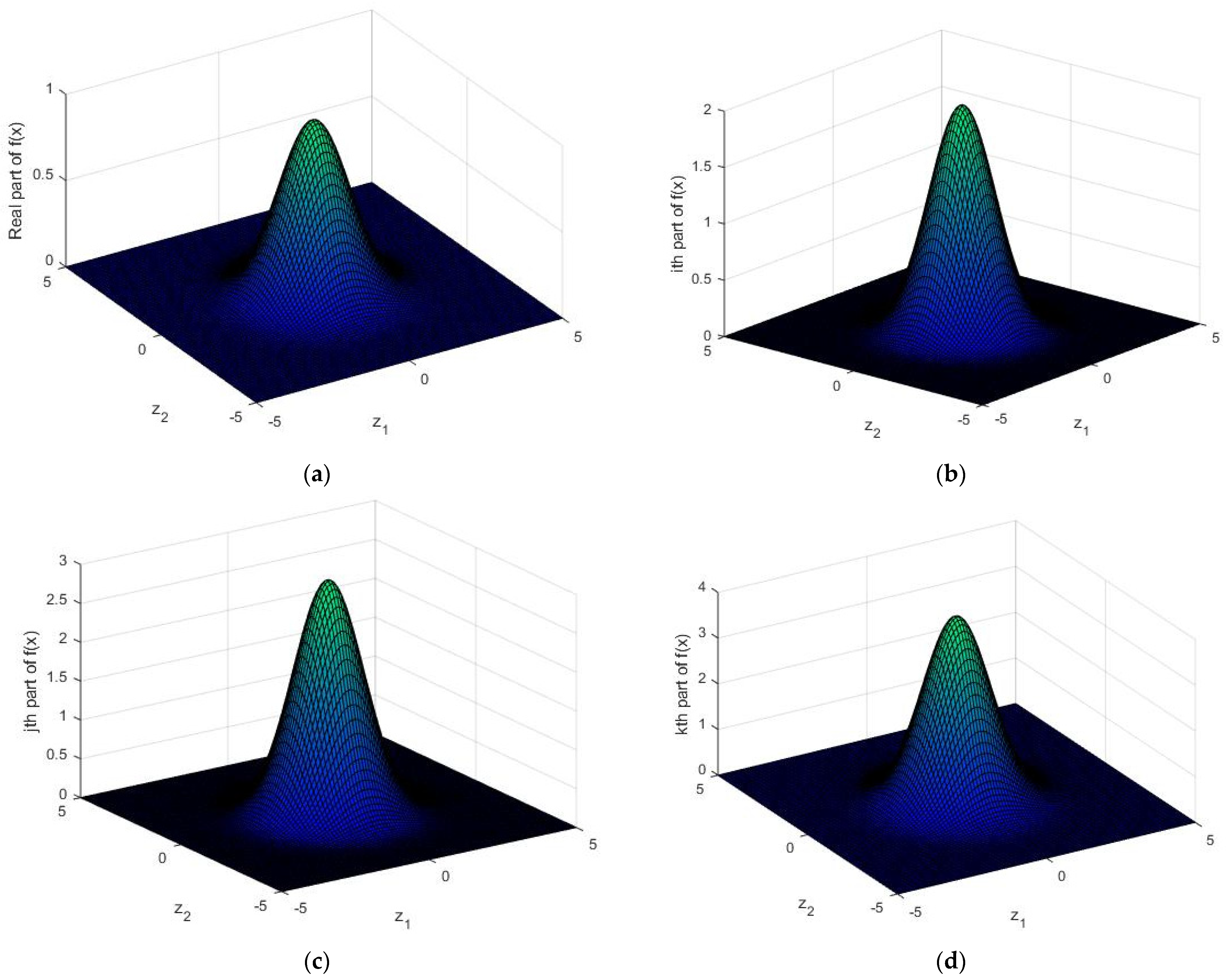
Consider the 2D quaternion-valued signal

$$f(\mathbf{z})=\left(1+2i+3j+4k\right)e^{\frac{-\left(z_1^2+z_2^2\right)}{2}}.$$

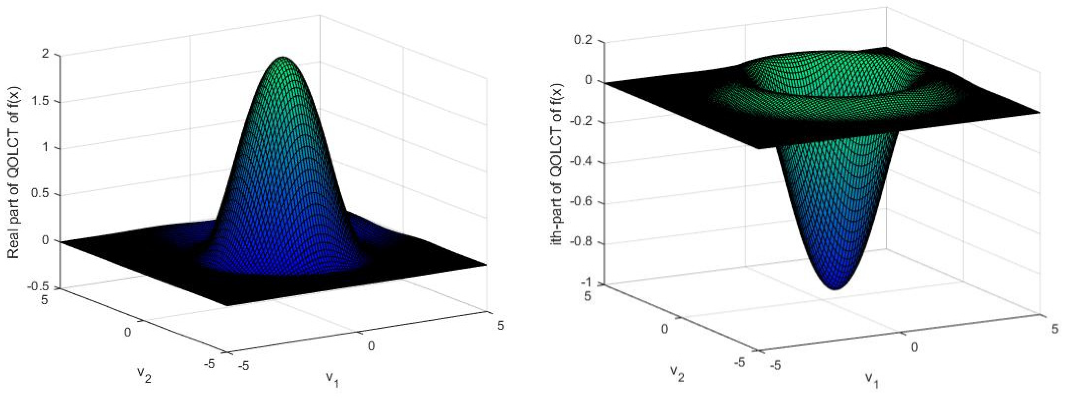
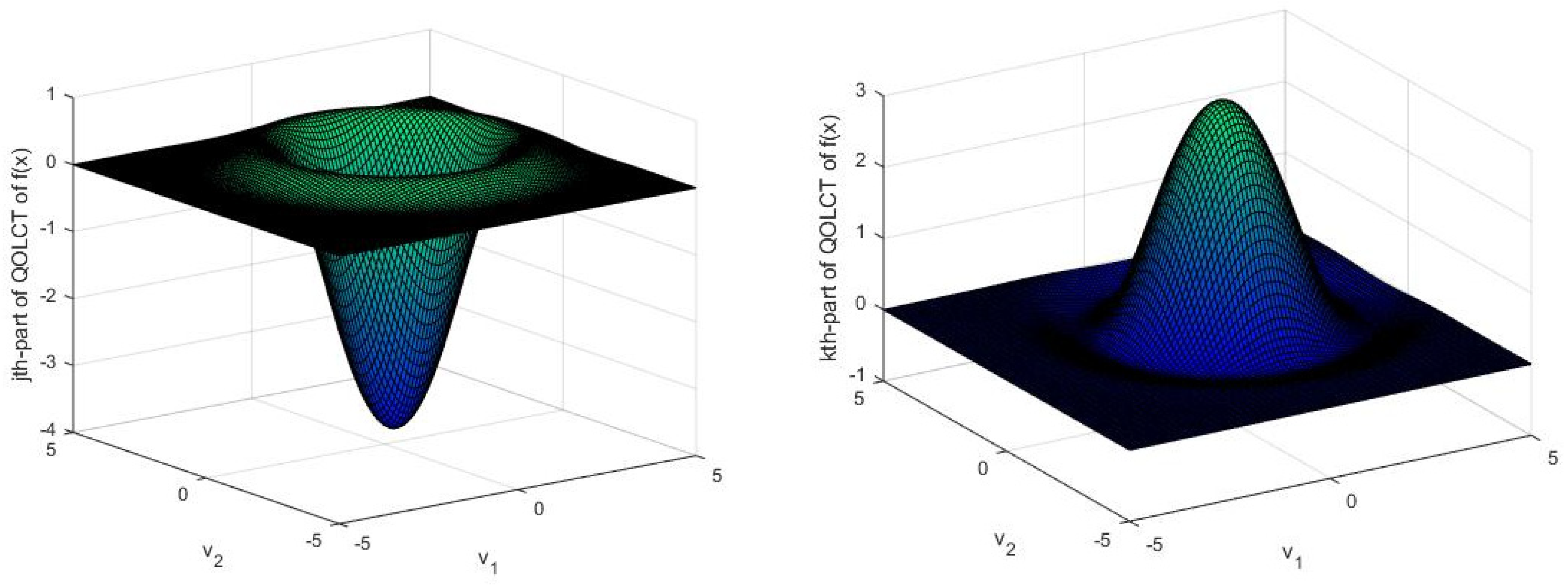
Then right-sided QOLCT of $f(\mathbf{z})$ is given by

$$\begin{array}{cc}\hfill & {}_R{\mathcal{O}}_{A_1,A_2}^{\mathbb{H},\mu }\left\{f\left(\mathbf{z}\right)\right\}\left(\mathbf{v}\right)\hfill \\ \hfill & ={\int }_{{\mathbb{R}}^2}\left(1+2i+3j+4k\right)e^{\frac{-\left(z_1^2+z_2^2\right)}{2}}{K}_{A_1}\left(z_1,v_1\right)K_{A_2}\left(z_2,v_2\right)d\mathbf{z}\hfill \\ \hfill & =\frac{\left(1+2i+3j+4k\right)}{2\pi \left(-1\right)\sqrt{b_1{b}_2}}\hfill \\ \hfill & \times exp\left\{\frac{1}{2b_1}\mu \left(-2v_1\left(d_1{\tau }_1-b_1{\eta }_1\right)+d_1\left(v_1^2+{\tau }_1^2\right)\right)+\frac{1}{2b_1}\mu \left(-2v_2\left(d_2{\tau }_2-b_2{\eta }_2\right)+d_2\left(v_2^2+{\tau }_2^2\right)\right)\right\}\hfill \\ \hfill & \times {\int }_{\mathbb{R}}exp\left\{-z_1^2\frac{\left(b_1-\mu a_1\right)}{2b_1}-\frac{z_1\mu \left(v_1-{\tau }_1\right)}{b_1}\right\}d{z}_1{\int }_{\mathbb{R}}exp\left\{-z_2^2\frac{\left(b_2-\mu a_2\right)}{2b_2}-\frac{z_2\mu \left(v_2-{\tau }_2\right)}{b_2}\right\}d{z}_2\hfill \\ \hfill & =\frac{\left(1+2i+3j+4k\right)}{2\pi \left(-1\right)\sqrt{b_1{b}_2}}exp\left\{\frac{\mu }{2}\left(\frac{-2v_1\left(d_1{\tau }_1-b_1{\eta }_1\right)+d_1\left(v_1^2+{\tau }_1^2\right)}{b_1}+\frac{-2v_2\left(d_2{\tau }_2-b_2{\eta }_2\right)+d_2\left(v_2^2+{\tau }_2^2\right)}{b_2}\right)\right\}\hfill \\ \hfill & \times \sqrt{\frac{2\pi b_1}{b_1-\mu a_1}}exp\left\{-\frac{{\left(v_1-{\tau }_1\right)}^2}{2b_1\left(b_1-\mu a_1\right)}\right\}\times \sqrt{\frac{2\pi b_2}{b_2-\mu a_2}}exp\left\{-\frac{{\left(v_2-{\tau }_2\right)}^2}{2b_2\left(b_2-\mu a_2\right)}\right\}\hfill \end{array}$$

$$\begin{array}{ll}=& -\left(1+2i+3j+4k\right)\exp \left\{\frac{\mu }{2}\left(\frac{-2v_1\left(d_1{\tau }_1-b_1{\eta }_1\right)+d_1\left(v_1^2+{\tau }_1^2\right)}{b_1}+\frac{-2v_2\left(d_2{\tau }_2-b_2{\eta }_2\right)+d_2\left(v_2^2+{\tau }_2^2\right)}{b_2}\right)\right\}\\ & \times \sqrt{\frac{1}{\left(b_1-\mu a_1\right)\left(b_2-\mu a_2\right)}}\exp \left\{-\frac{{\left(v_1-{\tau }_1\right)}^2}{2b_1\left(b_1-\mu a_1\right)}-\frac{{\left(v_2-{\tau }_2\right)}^2}{2b_2\left(b_2-\mu a_2\right)}\right\}.\end{array}$$

(17)

For computational convenience, we choose $A_1=A_2=\left(1,1,0,1,1,1\right)$ and imaginary unit $\mu =i,$ so that (17) yields

$$\begin{array}{cc}\hfill & {}_R{\mathcal{O}}_{A_1,A_2}^{\mathbb{H},\mu }\left\{f\left(\mathbf{z}\right)\right\}\left(\mathbf{v}\right)\hfill \\ \hfill & =-\left(1+2i+3j+4k\right)exp\left\{i\frac{\left(v_1^2+1\right)+\left(v_2^2+1\right)}{2}\right\}\frac{1}{\left(1-i\right)}exp\left\{-\frac{{\left(v_1-1\right)}^2+{\left(v_2-1\right)}^2}{2\left(1-i\right)}\right\}\hfill \\ \hfill & =-\left(1+2i+3j+4k\right)exp\left\{i\frac{\left(v_1^2+1\right)+\left(v_2^2+1\right)}{2}\right\}\frac{1}{\left(1-i\right)}exp\left\{-\frac{{\left(v_1-1\right)}^2+{\left(v_2-1\right)}^2}{4}\left(1+i\right)\right\}\hfill \\ \hfill & =-\frac{\left(1+2i+3j+4k\right)+\left(1+2i+3j+4k\right)i}{2}exp\left\{i\frac{\left(v_1^2+1\right)+\left(v_2^2+1\right)}{2}\right\}\hfill \\ \hfill & \times exp\left\{-i\frac{\left(v_1^2+1-2v_1\right)+\left(v_2^2+1-2v_2\right)}{4}\right\}exp\left\{-\frac{\left(v_1^2+1-2v_1\right)+\left(v_2^2+1-2v_2\right)}{4}\right\}\hfill \\ \hfill & =-\frac{\left(-1+3i+7j+k\right)}{2}exp\left\{i\frac{2\left(v_1^2+v_2^2+2\right)}{4}-i\frac{v_1^2+v_2^2-2\left(v_1+v_2\right)+2}{4}\right\}exp\left\{-\frac{v_1^2+v_2^2-2\left(v_1+v_2\right)+2}{4}\right\}\hfill \\ \hfill & =\frac{1-3i-7j-k}{2}exp\left\{i\frac{v_1^2+v_2^2-2\left(v_1+v_2\right)+2}{4}\right\}exp\left\{-\frac{v_1^2+v_2^2-2\left(v_1+v_2\right)+2}{4}\right\}\hfill \\ \hfill & =\frac{1-3i-7j-k}{2}\left(cos \alpha +i sin \alpha \right)e^{-\alpha },\hfill \end{array}$$

where $\alpha =\frac{v_1^2+v_2^2-2\left(v_1+v_2\right)+2}{4}.$

$$\begin{array}{ll}{}_R{\mathcal{O}}_{A_1,A_2}^{\mathbb{H},\mu }\left\{f\left(\mathbf{z}\right)\right\}\left(\mathbf{v}\right)\hfill & =\frac{\left(1-3i-7j-k\right)}{2}cos \alpha e^{-\alpha }+\frac{\left(1-3i-7j-k\right)i}{2}sin \alpha e^{-\alpha }\\ \hfill & =\frac{\left(1-3i-7j-k\right)}{2}cos \alpha e^{-\alpha }+\frac{\left(i+3+7k-j\right)}{2}sin \alpha e^{-\alpha }\hfill \\ \hfill & =\frac{1}{2}\left(cos \alpha +3sin \alpha \right)e^{-\alpha }+\frac{i}{2}\left(-3cos \alpha +sin \alpha \right)e^{-\alpha }\hfill \\ \hfill & +\frac{j}{2}\left(-7cos \alpha -sin \alpha \right)e^{-\alpha }+\frac{k}{2}\left(-cos \alpha +7sin \alpha \right)e^{-\alpha }.\hfill \end{array}$$

The graphical representation of the given quaternion-valued signal $f(\mathbf{z})$ is presented in Figure 2, whereas its right-sided QOLCT is depicted in Figure 3, for $A_1=A_2=\left(1,1,0,1,1,1\right)$ and $\mu =i.$

6.2. Application

The output of generalized swept-frequency filters is given by

$$\begin{array}{cc}h\left(\mathbf{z}\right)\hfill & =\left(f\left(\mathbf{z}\right){\otimes }^{A_1,A_2} g\left(\mathbf{z}\right)\left(e^{-\mu \frac{a_1}{2}{z}_1^2}{e}^{-\mu \frac{a_2}{2}{z}_2^2}{e}^{-\mu v_1\left(-{\eta }_1\right)}{e}^{-\mu v_2\left(-{\eta }_2\right)}\right)\right)e^{\mu \frac{a_1}{2}{z}_1^2}{e}^{\mu \frac{a_2}{2}{z}_2^2}{e}^{\mu v_1\left(-{\eta }_1\right)}{e}^{\mu v_2\left(-{\eta }_2\right)}\\ \hfill & =\left({\int }_{{\mathbb{R}}^2}f\left(\mathbf{z}-\mathbf{t}\right)g\left(\mathbf{t}\right)e^{-\mu \frac{a_1}{2}{t}_1^2}{e}^{-\mu \frac{a_2}{2}{t}_2^2}{e}^{-\mu v_1\left(-{\eta }_1\right)}{e}^{-\mu v_2\left(-{\eta }_2\right)}d\mathbf{t}\right)e^{\mu \frac{a_1}{2}{z}_1^2}{e}^{\mu \frac{a_2}{2}{z}_2^2}{e}^{\mu v_1\left(-{\eta }_1\right)}{e}^{\mu v_2\left(-{\eta }_2\right)},\hfill \end{array}$$

(18)

where $g\left(\mathbf{z}\right)$ is the impulse response of the shift-invariant filter. First, we choose the matrixes as $A_n=\left(a_n,1,-1,0,0,{\eta }_n\right),$ $n=1,2,$ and then take QOLCT from both sides of (18), we obtain

$$\begin{array}{l}{}_R{\mathcal{O}}_{A_1,A_2}^{ℍ,\mu }\left\{h\right\}\left(\mathbf{v}\right)\\ ={\displaystyle {\int }_{{ℝ}^4}f\left(\mathbf{z}-\mathbf{t}\right)g\left(\mathbf{t}\right)}{e}^{-\mu \frac{a_1}{2}{t}_1^2}{e}^{-\mu \frac{a_2}{2}{t}_2^2}{e}^{-\mu v_1\left(-{\eta }_1\right)}{e}^{-\mu v_2\left(-{\eta }_2\right)}\frac{1}{\sqrt{2\pi \mu }}\frac{1}{\sqrt{2\pi \mu }}{e}^{-\mu v_1{z}_1}{e}^{-\mu v_2{z}_2}d\mathbf{t}d\mathbf{z}\end{array}$$

Let $\mathbf{z}-\mathbf{t}=\mathbf{y},$ we have

$${}_R{\mathcal{O}}_{A_1,A_2}^{ℍ,\mu }\left\{h\right\}\left(\mathbf{v}\right)={\displaystyle {\int }_{{ℝ}^2}f\left(\mathbf{y}\right){}_R{\mathcal{O}}_{A_1,A_2}^{ℍ,\mu }\left\{g\right\}\left(\mathbf{v}\right)e^{-\mu v_1{y}_1}{e}^{-\mu v_2{y}_2}d\mathbf{y}}.$$

By decomposing $f\left(\mathbf{y}\right)$ as in (10), then by considering Definition 1, we arrive at the final result

$$\begin{array}{ll}{}_R{\mathcal{O}}_{A_1,A_2}^{ℍ,\mu }\left\{h\right\}\left(\mathbf{v}\right)=& {}_R{\mathcal{O}}_{A_1,A_2}^{ℍ,\mu }\left\{g\right\}\left(\mathbf{v}\right){}_R{\mathcal{F}}^{ℍ,\mu }\left\{f_0\right\}\left(\mathbf{v}\right)\\ & +i {}_R{\mathcal{O}}_{A_1,A_2}^{ℍ,\mu }\left\{g\right\}\left(\mathbf{v}\right){}_R{\mathcal{F}}^{ℍ,\mu }\left\{f_1\right\}\left(\mathbf{v}\right)\\ & +j {}_R{\mathcal{O}}_{A_1,A_2}^{ℍ,\mu }\left\{g\right\}\left(\mathbf{v}\right){}_R\mathcal{F}{}^{ℍ,\mu }\left\{f_2\right\}\left(\mathbf{v}\right)\\ & +k {}_R{\mathcal{O}}_{A_1,A_2}^{ℍ,\mu }\left\{g\right\}\left(\mathbf{v}\right){}_R\mathcal{F}{}^{ℍ,\mu }\left\{f_3\right\}\left(\mathbf{v}\right),\end{array}$$

(19)

where ${}_R{\mathcal{O}}_{A_1,A_2}^{ℍ,\mu }\left\{g\right\}\left(\mathbf{v}\right)$ is the transfer function of the generalized swept-frequency filter in the QOLCT domain. From (19), we see the use of QOLCT generalizes the treatment of swept-frequency filters.

7. Discussion

Overall, the idea to extend FT-related integral transforms to quaternion algebra is relatively new and constructed using the recipe: “take X (quaternions) and Y (transform) and make XY transform”. At first, it may be seen that there is not much of a difference between all these transforms, but the difference is significant and it is easily can be noticed from Figure 1. Moreover, the results and applications of all these transforms are not the same. For example, quaternion-valued optical systems with prisms or shifted lenses cannot be analyzed by QFT or QLCT because those transforms lack parameters that correspond to time shift and frequency modulation. Such problems, therefore, push us to study QOLCT, which has more parameters compared to other transforms.

Moreover, we would like to discuss why such transforms should be studied using color image processing as an example. Presently, we are surrounded by color images. Color image processing is a multidisciplinary topic that uses mathematical tools. With the rapid development of technologies, it seems that color imaging is well-studied at first. However, we still lack high-quality medical imaging, video calls, optical character recognition (e.g., converting scanned mathematical formulas into editable formulas), etc. One of the roles of mathematics here is to introduce new tools for engineering. With the proven advantage of QFT in color image processing [5,6] in this article we have introduced a new tool—right-sided QOLCT, which is more general than previously introduced tools and easily can be boiled down to its special cases. Additionally, QOLCT has a similar computational cost as the conventional QFT. Since images are defined over two dimensions our study object is 2D QOLCT. Regardless of optical and color image processing applications, QOLCT due to its advantage and flexibility can be also useful for a broad range of signal-processing applications such as object tracking and filter designing. The study of quaternion-valued OLCT is interesting and has a promising future in applications.

8. Conclusions

This article defines the most general form of QFT with more free parameters, the so-called 2D right-sided QOLCT. In other words, we extend the 2D right-sided QFT to the OLCT domain. The addition of the offset parameter in QOLCT enhances its flexibility and enables the input signal to be shifted within the quaternion domain. This feature can prove to be valuable in various signal-processing applications, including object tracking and image registration. Various properties of the 2D right-sided QOLCT, including linearity, additivity, translation, modulation, parity, inversion formula, and the Parseval theorem, are derived thoroughly. Furthermore, we obtain the convolution and correlation theorems related to QOLCT, which can be useful in engineering. Additionally, several forms of uncertainty principles for the 2D right-sided QOLCT are presented. First, we derive the Heisenberg-type uncertainty principle, and then we propose Pitt’s inequality for the 2D right-sided QOLCT. Moreover, by employing a sharp form of Pitt’s inequality and using the Parseval formula, we show the logarithmic uncertainty principle, which is a more general form of the Heisenberg uncertainty principle. Then, we give an example with illustrations to demonstrate the proposed 2D right-sided QOLCT and show its usage to study the generalized swept-frequency filters.

References

- Ell, T.A.; Le Bihan, N.; Sangwine, S.J. Quaternion Fourier Transforms for Signal and Image Processing; John Wiley & Sons: Hoboken, NJ, USA, 2014; pp. 35–66. [Google Scholar] [CrossRef]
- Hitzer, E. The quaternion domain Fourier transform and its properties. Adv. Appl. Clifford Algebras 2016, 26, 969–984. [Google Scholar] [CrossRef]
- Sangwine, S.J. The Discrete Quaternion Fourier Transform. In Proceedings of the Sixth International Conference on Image Processing and Its Applications, Dublin, Ireland, 14–17 July 1997. [Google Scholar] [CrossRef]
- Bayro-Corrochano, E.; Trujillo, N.; Naranjo, M. Quaternion Fourier descriptors for preprocessing and recognition of spoken words using images of spatiotemporal representations. J. Math. Imaging Vis. 2007, 28, 179–190. [Google Scholar] [CrossRef]
- Sangwine, S.J.; Ell, T.A. Hypercomplex Fourier transforms of color images. IEEE Trans. Image Process. 2001, 16, 137–140. [Google Scholar] [CrossRef]
- Bas, P.; Le Bihan, N.; Chassery, J.M. Color Image Watermarking Using Quaternion Fourier Transform. In Proceedings of the IEEE International Conference on Acoustics, Speech, and Signal Processing (ICASSP’03), Hong Kong, China, 6–10 April 2003. [Google Scholar] [CrossRef]
- Ouyang, J.; Coatrieux, G.; Shu, H.Z. Robust hashing for image authentication using quaternion discrete Fourier transform and log-polar transform. Digit. Signal Process. 2015, 41, 98–109. [Google Scholar] [CrossRef]
- Ell, T.A. Quaternion-Fourier Transforms for Analysis of Two-dimensional Linear Time-invariant Partial Differential Systems. In Proceedings of the 32nd IEEE Conference on Decision and Control, San Antonio, TX, USA, 15–17 December 1993. [Google Scholar] [CrossRef]
- Bahri, M.; Amir, A.K.; Resnawati; Lande, C. The quaternion domain Fourier transform and its application in mathematical statistics. IAENG Int. J. Appl. Math. 2018, 48, 184–190. [Google Scholar]
- Bahri, M.; Ashino, R. Duality Property of Two-sided Quaternion Fourier Transform. In Proceedings of the International Conference on Wavelet Analysis and Pattern Recognition (ICWAPR), Chengdu, China, 15–18 July 2018. [Google Scholar] [CrossRef]
- Cheng, D.; Kou, K.I. Generalized sampling expansions associated with quaternion Fourier transform. Math. Methods Appl. Sci. 2018, 41, 4021–4032. [Google Scholar] [CrossRef]
- Bahri, M. Product theorem for quaternion Fourier transform. Int. J. Math. Anal. 2014, 8, 81–87. [Google Scholar] [CrossRef]
- Pei, S.C.; Ding, J.J.; Chang, J.H. Efficient implementation of quaternion Fourier transform, convolution, and correlation by 2-D complex FFT. IEEE Trans. Signal Process. 2001, 49, 2783–2797. [Google Scholar] [CrossRef]
- Hitzer, E. Directional uncertainty principle for quaternion Fourier transform. Adv. Appl. Clifford Algebras 2010, 20, 271–284. [Google Scholar] [CrossRef]
- Chen, L.P.; Kou, K.I.; Liu, M.S. Pitt’s inequality and the uncertainty principle associated with the quaternion Fourier transform. J. Math. Anal. Appl. 2015, 423, 681–700. [Google Scholar] [CrossRef]
- Lian, P. Uncertainty principle for the quaternion Fourier transform. J. Math. Anal. Appl. 2018, 467, 1258–1269. [Google Scholar] [CrossRef]
- Xu, G.L.; Wang, X.T.; Xu, X.G. Fractional quaternion Fourier transform, convolution and correlation. Signal Process. 2008, 88, 2511–2517. [Google Scholar] [CrossRef]
- Bahri, M.; Ashino, R. Two-dimensional quaternion linear canonical transform: Properties, convolution, correlation, and uncertainty principle. J. Math. 2019, 2019, 1062979. [Google Scholar] [CrossRef]
- Li, Z.W.; Gao, W.B.; Li, B.Z. A new kind of convolution, correlation and product theorems related to quaternion linear canonical transform. SIViP 2021, 15, 103–110. [Google Scholar] [CrossRef]
- Kou, K.I.; Ou, J.; Morais, J. Uncertainty principles associated with quaternionic linear canonical transforms. Math. Methods Appl. Sci. 2016, 39, 2722–2736. [Google Scholar] [CrossRef]
- Zhang, Y.N.; Li, B.Z. Novel uncertainty principles for two-sided quaternion linear canonical transform. Adv. Appl. Clifford Algebras 2018, 28, 15. [Google Scholar] [CrossRef]
- Urynbassarova, D.; Teali, A.A.; Zhang, F. Discrete quaternion linear canonical transform. Digit. Signal Process. 2022, 122, 103361. [Google Scholar] [CrossRef]
- Shah, F.A.; Teali, A.A.; Tantary, A.Y. Linear canonical wavelet transform in quaternion domains. Adv. Appl. Clifford Algebras 2021, 31, 42. [Google Scholar] [CrossRef]
- Bhat, Y.A.; Sheikh, N.A. Quaternionic linear canonical wave packet transform. Adv. Appl. Clifford Algebras 2022, 32, 43. [Google Scholar] [CrossRef]
- Srivastava, H.M.; Shah, F.A.; Teali, A.A. Short-time special affine Fourier transform for quaternion-valued functions. Rev. Real Acad. Cienc. Exactas Fis. Nat. Ser. A-Mat. 2022, 116, 66. [Google Scholar] [CrossRef]
- Pei, S.C.; Ding, J.J. Eigenfunctions of the offset Fourier, fractional Fourier, and linear canonical transforms. J. Opt. Soc. Am. A 2003, 20, 522–532. [Google Scholar] [CrossRef] [PubMed]
- Stern, A. Sampling of compact signals in the offset linear canonical domains. Signal Image Video Process. 2007, 1, 359–367. [Google Scholar] [CrossRef]
- Urynbassarova, D.; Urynbassarova, A.; Al-Hussam, E. The Wigner-Ville Distribution based on the Offset Linear Canonical Transform domain. In Proceedings of the 2nd International Conference on Modeling, Simulation and Applied Mathematics (MSAM2017), Advances in Intelligent Systems Research, Bangkok, Thailand, 26–27 March 2017. [Google Scholar] [CrossRef]
- Urynbassarova, D.; Li, B.Z.; Tao, R. Convolution and correlation theorems for Wigner-Ville distribution associated with the offset linear canonical transform. Optik 2018, 157, 455–466. [Google Scholar] [CrossRef]
- Xu, S.; Chen, Z.; Zhang, K.; He, Y. Aliased polyphase sampling theorem for the offset linear canonical transform. Optik 2020, 200, 163410. [Google Scholar] [CrossRef]
- Shah, F.A.; Teali, A.A.; Tantary, A.Y. Windowed special affine Fourier transform. J. Pseudo-Differ. Oper. Appl. 2020, 11, 1389–1420. [Google Scholar] [CrossRef]
- Urynbassarova, D.; Urynbassarova, A. Hybrid transforms. In Fourier Transform and Its Generalizations; Working Title; Bhat, M.Y., Ed.; IntechOpen: London, UK, 2022. [Google Scholar] [CrossRef]
- Shah, F.A.; Teali, A.A. Scaling Wigner distribution in the framework of linear canonical transform. Circuits Syst. Signal Process. 2023, 42, 1181–1205. [Google Scholar] [CrossRef]
- El Kassimi, M.; El Haoui, Y.; Fahlaoui, S. Wigner-Ville distribution associated with the quaternion offset linear canonical transform. Anal. Math. 2019, 45, 787–802. [Google Scholar] [CrossRef]
- Zhu, X.; Zheng, S. Uncertainty principles for the two-sided offset quaternion linear canonical transform. Math. Methods Appl. Sci. 2021, 44, 14236–14255. [Google Scholar] [CrossRef]
- Bahri, M.; Karim, S.A.A. Pitt’s inequality for offset quaternion linear canonical transform. In Intelligent Systems Modeling and Simulation II. Studies in Systems, Decision and Control; Karim, S.A.A., Ed.; Springer: Berlin/Heidelberg, Germany, 2022; pp. 409–419. [Google Scholar] [CrossRef]
- Bhat, M.Y.; Almanjahie, I.M.; Dar, A.H.; Dar, J.G. Wigner-Ville distribution and ambiguity function associated with the quaternion offset linear canonical transform. Demonstr. Math. 2022, 55, 786–797. [Google Scholar] [CrossRef]
- Urynbassarova, D.; El Haoui, Y.; Zhang, F. Uncertainty principles for Wigner-Ville distribution associated with the quaternion offset linear canonical transform. Circuits Syst. Signal Process. 2023, 42, 385–404. [Google Scholar] [CrossRef]
- Folland, G.B.; Sitaram, A. The uncertainty principle: A mathematical survey. J. Fourier Anal. Appl. 1997, 3, 207–238. [Google Scholar] [CrossRef]
- Beckner, W. Pitt’s inequality and the uncertainty principle. Proc. Am. Math. Soc. 1995, 123, 1897–1905. [Google Scholar] [CrossRef]