
Stability of Traveling Fronts in a Neural Field Model

1
Department of Neurosurgery, Perelman School of Medicine, University of Pennsylvania, Philadelphia, PA 19104, USA
2
Department of Mathematics, College of Arts and Sciences, Drexel University, Philadelphia, PA 19104, USA
*
Author to whom correspondence should be addressed.
†
These authors contributed equally to this work.
Mathematics 2023, 11(9), 2202; https://doi.org/10.3390/math11092202
Submission received: 29 March 2023
/
Revised: 26 April 2023
/
Accepted: 4 May 2023
/
Published: 7 May 2023
(This article belongs to the Special Issue Complexity in Human-Computer Interfaces: Information-Theoretic Approaches and Beyond)
Abstract
:We investigate the stability of traveling front solutions in the neural field model. This model has been studied intensively regarding propagating patterns with saturating Heaviside gain for neuron firing activity. Previous work has shown the existence of traveling fronts in the neural field model in a more complex setting, using a nonsaturating piecewise linear gain. We aimed to study the stability of traveling fronts in the neural field model utilizing the Evans function. We attained the Evans function of traveling fronts using an integration of analytical derivations and a computational approach for the neural field model, with previously uninvestigated piecewise linear gain. Using this approach, we are able to identify both stable and unstable traveling fronts in the neural field model.
MSC:
34L161. Introduction
There is extensive biological evidence supporting the existence of traveling front phenomena in the brain [1,2,3,4,5,6,7]. The coarse-grained average activity of a neural network can be explained with the network equation first presented by Amari [8]:
Without loss of generality, we can set the synaptic decay time . We also have that is the synaptic input to neurons located at position at time , and this represents the level of excitation or amount of input into a neural element. The coupling function determines the connections between neurons. The nonnegative and monotonically nondecreasing gain function denotes the firing rate at x at time t.
Ermentrout and McLeod [9] considered a singular network of excitatory neurons distributed on a real one-dimensional line. They showed that there is a unique and asymptotically stable monotonic traveling front solution. This front joins the stable constant solutions and . They also explicitly solved the integral equation for the limiting case when is the Heaviside function.
Zhang investigated the existence and stability of traveling front solutions of (1) with the Heaviside gain function and a coupling function that is even, nonnegative, and piecewise smooth [10]. He derived the integral Evans function for an associated eigenvalue problem resulting from linearization (1) around the front . Using the Evans function , he further proved that the real part of the eigenvalue cannot be nonnegative, except for the simple eigenvalue , which is associated with translational invariance. Therefore, he concluded that the traveling fronts of (1) are linearly stable.
Guo showed the existence of nonmonotonic traveling front solutions of (1) with a “Mexican hat” type of lateral inhibition coupling and nonsaturating piecewise linear gain [11]. She also established an ODE formulation, to compute the point spectrum on the right half of the complex plane for traveling front solutions of (1) with a “Mexican hat” type of lateral inhibition coupling function and Heaviside gain function.
In 2004, Coombes and Owen showed how to construct Evans functions for several integral neural field equations [12]. In this work, the analysis was performed with a Heaviside firing rate function, which allowed them to construct several explicit forms of Evans function for several types of integral neural field equations. We will be able to expand on this work by investigating Evans functions with a non-Heaviside firing rate function.
There have been various studies on traveling fronts for Amari’s neural field model in the recent past, as well as in current work. For example, in 2012, Coombes, Schmidt, and Bojak analyzed a two-dimensional neural field model with Heaviside gain [13]. They investigated the stability of stationary fronts and determined the conditions for which stability is achieved. In 2016, Coombes and Liang investigated traveling fronts in a stochastic neural field model using Heaviside gain with exponentially decaying spatial interactions and threshold noise, and they were able to find several stability branches for the fronts [14]. In 2017, Coombes, Avitabile, and Gökçe considered a two-dimensional neural field model with Heaviside gain and imposed Dirichlet boundary conditions and conducted a stability analysis [15]. They were also able to verify their theoretical findings with computational results. More recently, in 2022, Cook, Peterson, Woldman, and Terry analyzed and derived the relationships and formulations of several relevant neural field models, including Amari’s with Heaviside gain [16]. They reported several modern formulations of neural field modeling, as well as its important connection to clinical applications. Also in 2022, Qin, Fu, Jin, and Peng used the neural field model with arctangent gain to compare with experimental data obtained clinically [17]. They were able to determine that the neural field model was able to effectively model real-world data more robustly than some other respected representations. Earlier in 2023, González-Ramírez investigated the existence of traveling fronts in fractional-order formulations of the neural field model with Heaviside gain [18]. Evidently, we can see that Amari’s work is still highly relevant in contemporary times.
We aim to extend the work of Ermentrout and McLeod, Zhang, and Guo’s previous studies by analyzing the problem with nonsaturating gain. This will involve linearizing the traveling front solution, to set up an eigenvalue problem. We then derive the equivalent ODE of the eigenfunction, analyzing both real and imaginary components, to set up a system of ODEs. Finally, we compute the Evans function for the system and conclude, through computation, the stability, by using the Evans function. All numerical and symbolic calculations in this paper were performed using Mathematica, and all visualizations were carried out using Python.
2. Materials and Methods
In this section of the paper, we introduce some of the functions that will be utilized in the neural field model. We then linearize the neural field model for a perturbed solution and derive ordinary differential equations equivalent to the linearized stability integrodifferential equation. Next, we derive the matching conditions for where the front crosses the threshold. We conclude by identifying possible forms for the resulting eigenfunction and then deriving the Evans function that will be used for the stability analysis.
2.1. Coupling Function, Gain Function, and Front Solutions Considered
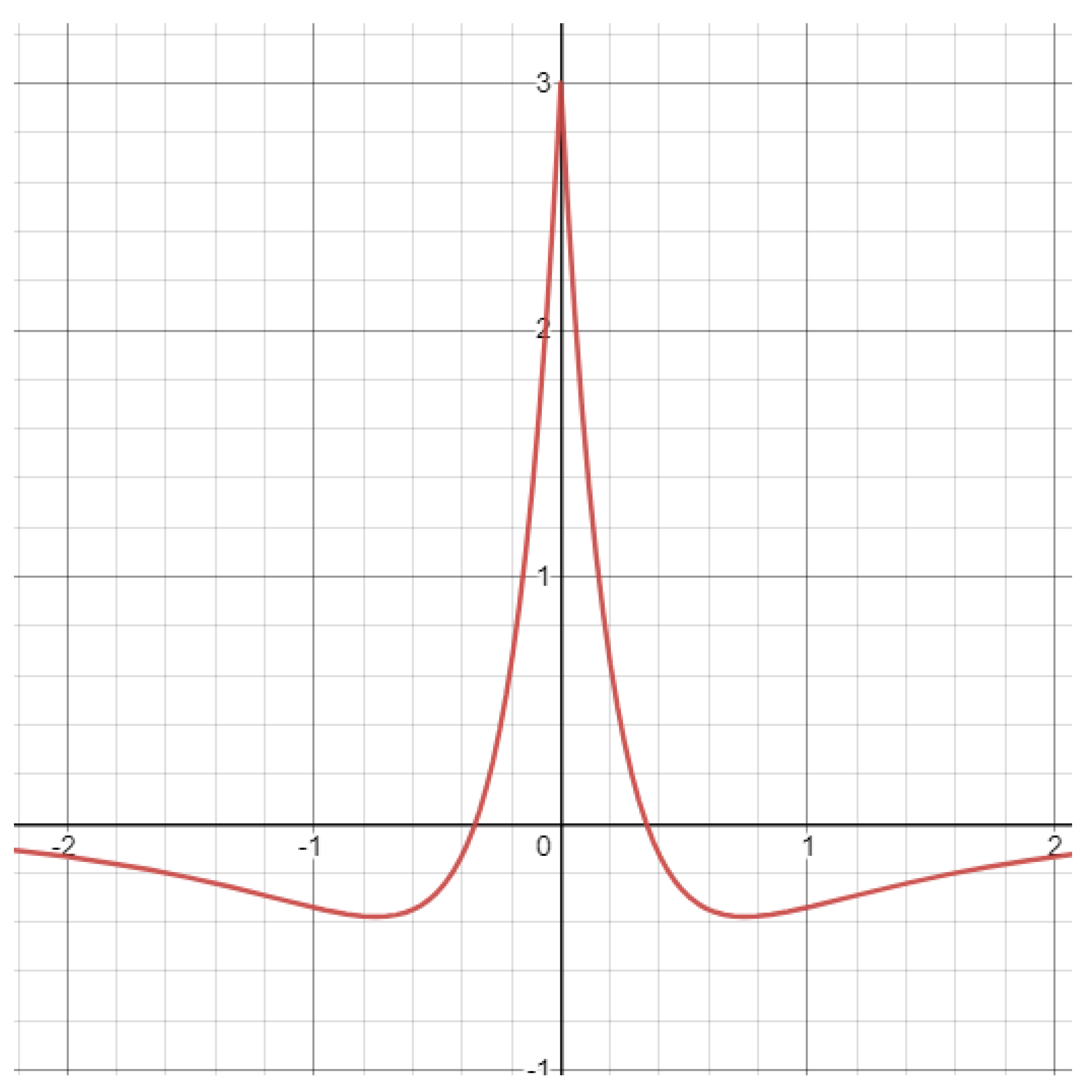
We begin by discussing some of the functional parameters in our model. We will use a coupling function similar to the one previously used by Guo, the so-called Mexican hat function [11]. This function can be constructed using a variety of exponential functions. For our demonstration, we will consider a function of the form
where we require that and , in order to satisfy the properties of the coupling function used in these networks, in addition to the other following conditions:
- on an interval , and ,
- is decreasing on ,
- on ,
- is continuous on , and is integrable on ,
- has a unique minimum on such that , and is strictly increasing on .
This function resembles a Mexican hat, except it has a cusp at the maximum of the function, as opposed to a smooth curve [12]. Other lateral inhibition coupling functions chosen are the Gaussian type [8], as well as the oscillatory types presented in [19,20]. Here, and . The area above the x-axis represents the net excitation in the network, while the area below the x-axis represents the net inhibition in the network. If then excitation dominates the network, and if , inhibition dominates. An example of this type of function is shown in Figure 1.
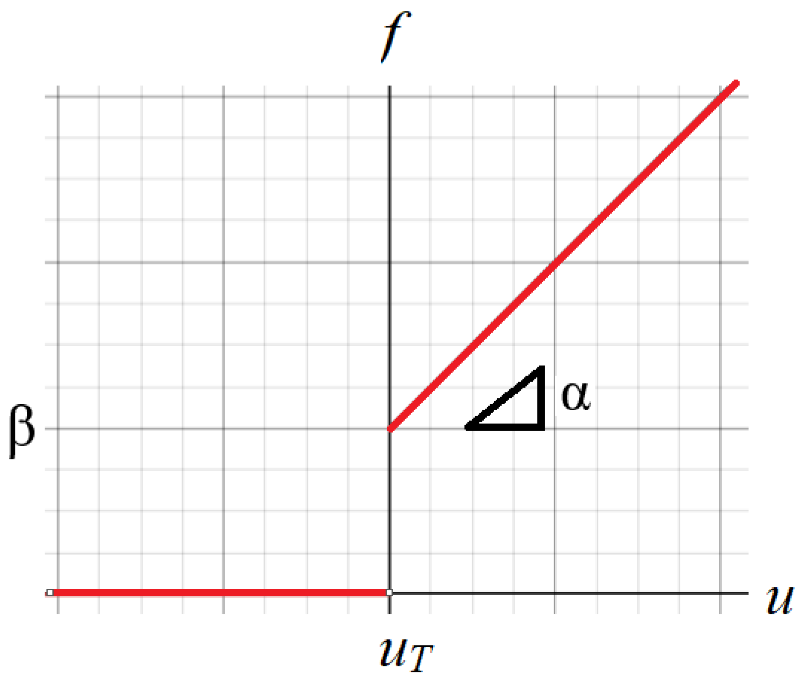
The next function we must consider is the gain function. Here, we consider a gain function of the following type:
where is the Heaviside gain function:
Here, represents the threshold. The gain function (3) does not saturate with a positive slope . Without loss of generality, we set . Note that the gain function (3) turns into the Heaviside function when . Stability was investigated for this case in [11] and others. We extend this work by examining the stability when . A graph of the gain function is seen in Figure 2.
The traveling front solution can be described by first rewriting the neural field equation in the traveling coordinate , where c is the traveling velocity:
We are interested in finding traveling front solutions that connect the two constant solutions of (4), which are and where we have that In the lateral inhibition network, we set in order to normalize In other words, we then want a traveling front that connects and .
Since the network given by (4) is translation invariant, the traveling front can cross the threshold h at any finite value of . We will, without loss of generality, assume that , on , and on . Therefore, we define the traveling front solution as follows:
where and are bounded and continuous on . The nth order (for ) derivatives of u are continuous everywhere, with the exception of at . The solution also satisfies
and also
The existence of this front solution and its forms were proven in [11]. We find that there are six possible types of front that we will analyze the stability for. In the following cases, the represent eigenvalues of the associated characteristic equation of the ordinary differential equations that represent the traveling fronts.
Positive Velocity : In the first three cases, on . On , has the following forms:
Case L1: All five with and , then
where is a constant, and since , we find that .
Case L2: Three with , , and with . Then,
Case L3: We have with , and four complex , such that with and with . Then,
Negative Velocity : In the next three cases, on . On , has the following forms:
Case L4: All five with and , then
Case L5: Three with with , , and . Then,
Case L6: We have with , and four complex , such that with and with . Then,
Each of these cases allows for different domains for the parameters h and . We refer the interested reader to [11] for the details on how these may be obtained, as well as the derivation of these six cases.
2.2. Formation of the 5th Order ODE
In order to investigate the stability of the traveling front solution, we introduce a perturbation. We perturb the traveling front solution with with small , where , and where , i.e., .
The function belongs to the set , where both and are bounded, continuous, and complex-valued integrable complex-valued functions defined on
. After perturbing the front solution, we now employ the method of linearization. By taking
we can linearize the front solution via introducing the perturbed front solution and Taylor expanding to order .
The resulting eigenvalue equation is given by
In the derivations needed for the stability analysis, we will study the eigenvalue Equation (6). In this equation, we note a Heaviside function in the integral term. As a result, when , we lose the integral term, and the equation becomes
This necessitates studying the relevant details in separate domains, one being and the other being .
Theorem 1.
The equivalent fifth order linear ODE for Equation (6) on
is:
or equivalently,
Proof.
For the above threshold values, we must incorporate the integral term of (6).
Theorem 2.
2.3. Matching Conditions for the ODE
Before deriving the matching conditions for the ODE, we present a lemma on the integral term that appears in the derivation, to simplify the presentation of the matching conditions. This will allow us to closely analyze the integral term where the threshold and resulting discontinuity occur.
Lemma 1.
When analyzing the matching conditions for the equivalent ODEs of the eigenvalue Equation (6), the integral term
has the following matching conditions at :
Proof.
First, we observe that I is necessarily continuous, as its integrand is Lebesgue integrable, which gives us the equality (16a).
To see (16b), we first proceed by writing I as
In addition, we let
and
Next, we take the derivative using the Leibniz integral rule. We observe that
Since the integrands are once again continuous, we see that
The proofs for (16c) and (16d) are similar, but much more cumbersome in detail, and we present these details in Appendix A. □
We are now prepared to derive the matching conditions to join the eigenfunction at .
Theorem 3.
The matching conditions for the eigenfunction at are as follows:
Proof.
In particular, we note that , with a similar result for , so that we may make the substitutions and from the previous lemma.
To see matching condition (19), we differentiate (6) with respect to and rearrange to obtain the following:
where
Now, since
we note that
Now, we determine that
and
Using the previous lemma, we have that is continuous at , so taking gives (19) as needed.
Contrarily to before, we note that
Thus, in this case, is continuous at . We can then calculate,
and
The previous lemma gives us
The same technique can be used to show (21). □
2.4. Forms for Eigenfunction
Next, we must discuss the forms for our eigenfunction, ; the solution to the ODE given by (7) and (12). This will be very similar to the forms for the traveling front itself, as seen in [11].
The characteristic values for (7) are and . To have an equation that converges to 0 at , the eigenfunction must be in one of the following forms
in the case where (recall ).
If , then we cannot have or , since . First, we analyze the term using Euler’s formula:
We must consider the fact that coefficients of complex terms may have a real and imaginary component, i.e., with . As a result, we find that if , then:
In conclusion, we find that when , the eigenfunction is given by
When , we must determine the form of by first referencing (12), which depends on the roots of the following characteristic equation that is a polynomial of degree five:
Unfortunately, the roots of the polynomial (32) now depend on the value of . We cannot solve the equation without knowing , and there is no explicit form for the roots of a fifth degree polynomial. However, we can use the discriminant, , to determine the explicit solution form of the eigenfunction.
We can find the discriminant as follows: first, we find the resultant of the characteristic equation. When we consider (32), and its derivative given by
we can then form the Sylvester matrix below. The Sylvester matrix is then divided by c, the leading term, to give the discriminant [21].
In this case, the matrix is given by
where , , , , , and , which are, of course, the coefficients in (32) and (33). Again, by calculating , we find the discriminant of (34).
In the case where , there are either five real characteristic values or four complex values with one real characteristic value when the discriminant . There are two complex and three real characteristic values when . Finally, there are repeated roots when .
If , we will obtain 5 complex , which, in general, are not pairwise conjugate pairs. An interesting observation about the roots of the characteristic equations is given by the following lemma:
Lemma 2.
This lemma provides some insight into the structure of the eigenfunction when . We can now give the eigenfunction structure. We show the eigenfunction forms both for when and . Due to the nature of the roots of real and complex polynomials, we can more explicitly represent the eigenfunction when . When , we cannot explicitly write out the eigenfunction, as it will depend on complex roots of the complex characteristic polynomial (12) when . We describe the structure for both of these cases in the following two sections.
2.4.1. Eigenfunction Forms When ()
When , (), we obtain the following structure:
: In the first four cases, on . On , has one of the following forms:
Form 1: All five with and , then
Form 2: Three with , , and with . Then,
Form 3: Three with with , , and . Then,
Form 4: We have with , and four complex such that with and with . Then,
In the next four cases, on . On , has one of the following forms:
Form 5: All five with and , then
Form 6: Three with , and with . Then,
Form 7: Three with with , , and . Then,
Form 8: We have with , and four complex such that with and with . Then,
Form 9: When there are repeated roots of (32). This happens only at a few isolated values of , and it may occur for both and .
- If , then is the transition between either cases 1 and 2, cases 2 and 4, or cases 3 and 4.
- For the first two transitions mentioned above, the repeated roots are . The solution form is
- If the transition is between case 3 and case 4, the solution form is the same as case 3.
- If , then is the transition between either cases 4 and 5, cases 6 and 8, or cases 7 and 8.
- For the transition from 4 to 5 or 6 to 8, the repeated roots are . The solution form is the same as case 6.
- For the transition from 7 to 8, the solution form is the same as case 7.
Finally, when , there is a stationary front, where we use the following ODEs:
This will occur for some and h values in the range that we consider.
2.4.2. Eigenfunction Forms When ()
If (), the form of the eigenfunction will resemble Cases 3 and 4 in the () case. Again, we recall that , and the analysis is similar to (29). We find that, when , the eigenfunction takes the form given by
where we leave each term in its factored form for the sake of space.
We note that all of these solution form cases are possible within each of the stability investigations for the front cases of L1, L2, L3, L4, L5, and L6, as outlined in [11]. All of the relevant cases are obtained by finding the appropriate eigenvalues of the characteristic equation for each type of front in Mathematica.
2.5. Evans Function for Stability Analysis
In the stability analysis for , we need to proceed differently from Zhang’s, Guo’s, and Coombes’ and Owen’s previous approaches. However, similarly to their previous analyses, we claim that the determinant of our coefficient matrix of the system formed by our matching conditions will represent the Evans function. One of the main differences here is that we will not be able to explicitly represent the Evans function as in [12]. Instead, we will rely on a computational approach. Another important consideration here is that the Evans function is specific to each traveling front. We first determine the traveling front equation. This allows us to obtain the required parameter values for the stability eigenfunction. By varying across a discretized domain, we can calculate the values of the Evans function. This will allow us to find the necessary eigenvalues and determine the stability of the traveling front.
First, we will formally state the necessary conditions for the Evans function.
Theorem 4.
Theorem of Evans: The Evans function is a complex analytic function, and it is real-valued if the eigenvalue parameter λ is real. The complex number λ is an eigenvalue of the operator if, and only if, . Moreover, the algebraic multiplicity of an eigenvalue is exactly equal to the order of the zero of the Evans function. (from [22,23,24,25]).
The discrete spectrum of an operator is defined as all , such that the resolvent operator does not exist, or equivalently, where for all . It should be noted that, in order to confirm that the discrete spectrum, and thus our Evans function, is the only source of possible instability, the essential spectrum has previously been shown to be on the line for for all traveling fronts we consider [10,26]. As a result, only the discrete spectrum, the zeroes of the Evans function , will contribute to the stability analysis for each front.
To begin, we need to define our operator, which we will denote as . First, recall the eigenvalue Equation (6)
We follow the previous analysis by [10,11,26] and others. By letting
our eigenvalue equation becomes
Here, is a linear operator defined on a Banach space of functions that are continuous, bounded, and decay exponentially as .
In this case, the function is complex-valued, and will, of course, lead to a complex-valued Evans function.
First, recall the matching conditions:
Now, this system, along with the corresponding form of the eigenfunction (which varies as is varied), forms a system in terms of coefficients through since and are expressed in terms of (presented in the previous section). We can represent this as a matrix equation:
where is the coefficient matrix and is the column vector of ’s with (). We describe the procedure for obtaining , as well as provide some examples of in Appendix B. We also include an explicit form for when in Appendix C. Unfortunately, no explicit solution for exists when . Note that we can use either the above or below threshold equations to calculate in the matching conditions, since they are defined as equal at this point. There exists a nontrivial solution to (38) if, and only if, the matrix has where represents the determinant of the matrix . Therefore, we let . We note that the Evans function will have a real and imaginary component, and the zeroes of this function will occur when
We can locate the values for that satisfy (39) using the intersections of the zero-level contours of the real and imaginary components of . We must be careful in our analysis, since the eigenfunction undergoes structural changes as we vary . Its form depends on solutions to the characteristic equation for (6), which varies depending on the choice of . We stress once more that the Evans function cannot be represented explicitly, and we can only numerically compute . Furthermore, we can only determine the values of that solve (39) numerically. We go through some examples of this analysis in the next section.
3. Results
In this section, we examine the computational results of the stability analysis for each of the six cases presented in Section 2. We find that the positive speed fronts we analyze are stable, a small magnitude negative speed front is stable, and two additional negative speed fronts are unstable. All calculations were performed with Mathematica, and all plots were created using Python’s matplotlib package. Depending on the desired accuracy and performance, the mesh size typically used was and , although larger values were sometimes used for areas of low stability activity, and smaller values were sometimes used for areas of high stability activity, to capture all relevant details. We now examine the individual cases.
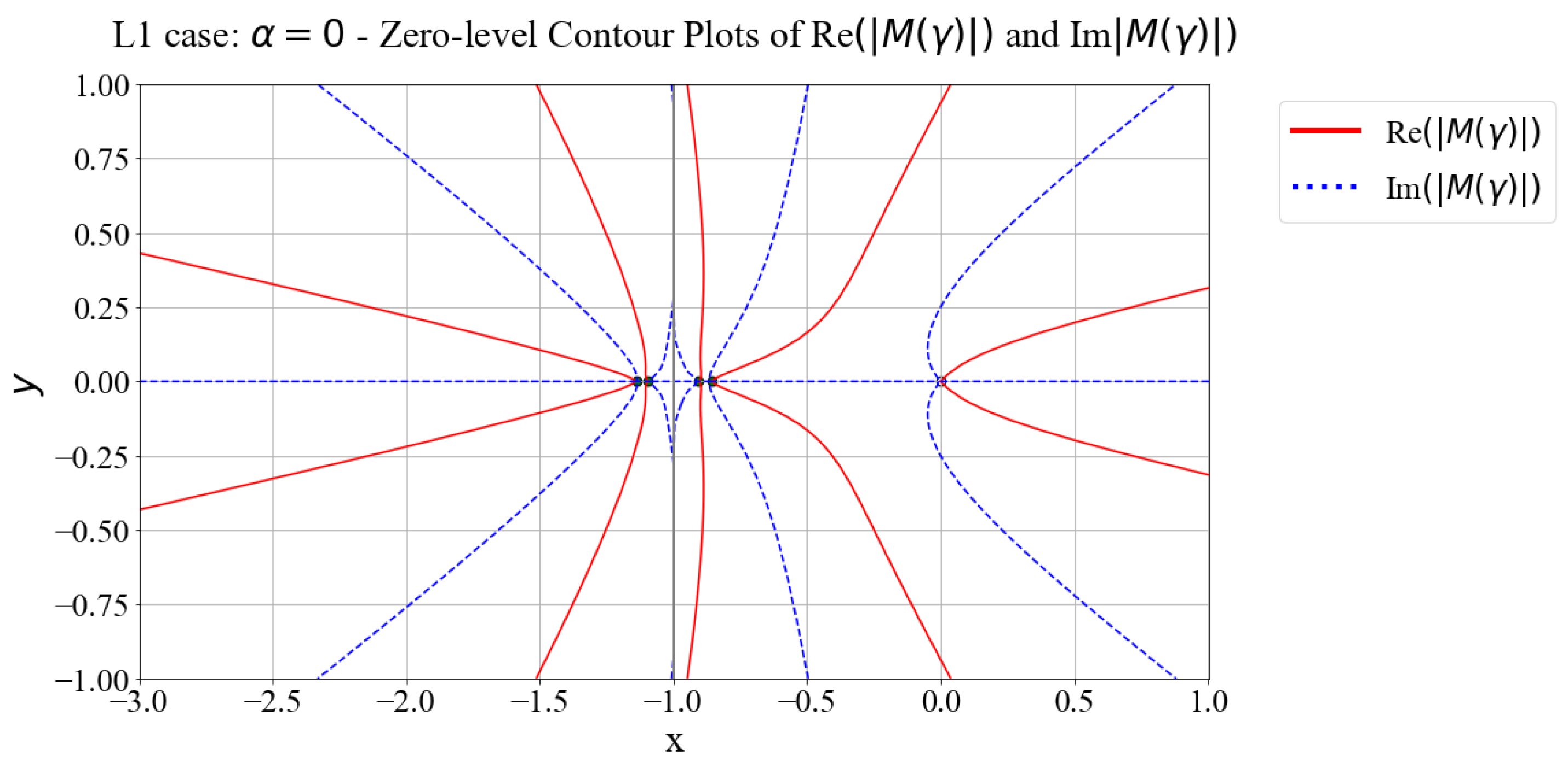
3.1. Case L1 Analysis
First, we analyze two examples for the L1 case, with parameters given in the caption of each figure. Recall that this case indicates that we have a traveling front with all real eigenvalues and a positive traveling speed c. We will consider two fronts, one where , as well as . Unless otherwise stated, we assume that and in for all cases.
We first investigate when and . After finding the front solution, we can find the zeroes of the Evans function, which are the zeroes of the determinant of the matching conditions matrix given by (38). We find through computation that the zeroes are the gamma values of approximately , , , , and . We find that since all values of such that are negative, we conclude that this particular front is linearly stable. We show this below in Figure 3.
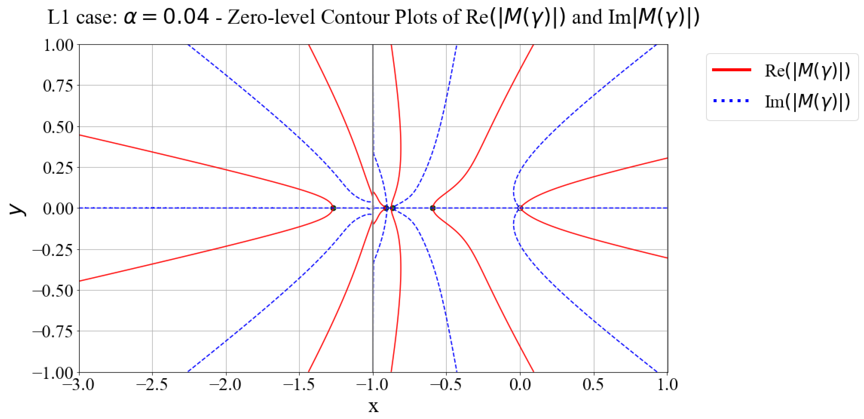
Next, we analyze when and . We find through computation that the zeroes are the gamma values of approximately , , , , and . Since all values of such that are negative, we conclude that this particular front is linearly stable. We show this below in Figure 4.
3.2. Case L2 Analysis
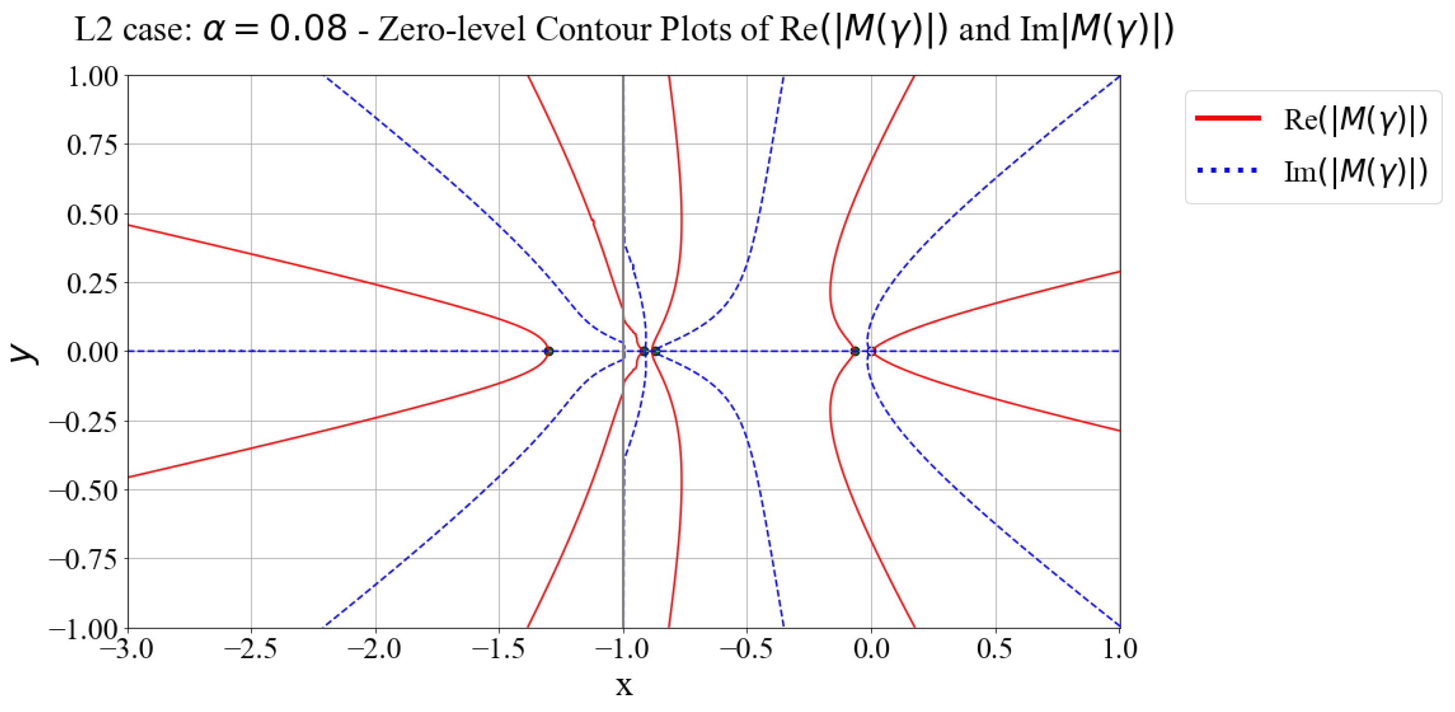
Next, we analyze an example for the L2 case. Recall that this case indicates that we have a traveling front with one conjugate pair of complex eigenvalues and three real eigenvalues and a positive traveling speed c. In this example, we take and .
We find through computation that the zeroes are the gamma values of approximately , , , , and . Since all values of such that are negative, we conclude that this front is linearly stable. We show this below in Figure 5.
3.3. Case L3 Analysis
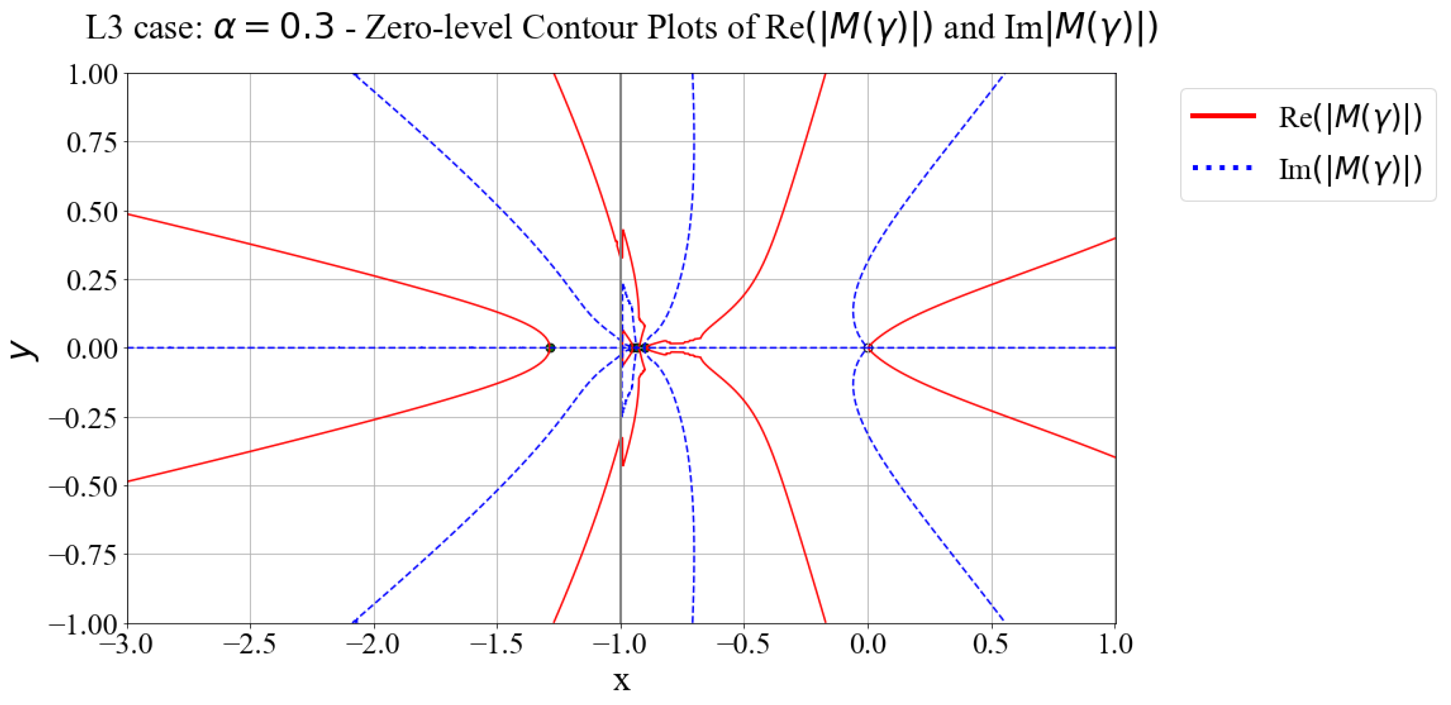
Next, we analyze an example in the L3 case. Recall that this case indicates that we have a traveling front with two conjugate pairs of complex eigenvalues and one real eigenvalue and a positive traveling speed c. In this example, we will use and .
We find through computation that the zeroes are the gamma values of approximately , , , , and . Since all values of such that are negative, we conclude that this particular front is linearly stable. We show this below in Figure 6.
3.4. Case L4 Analysis
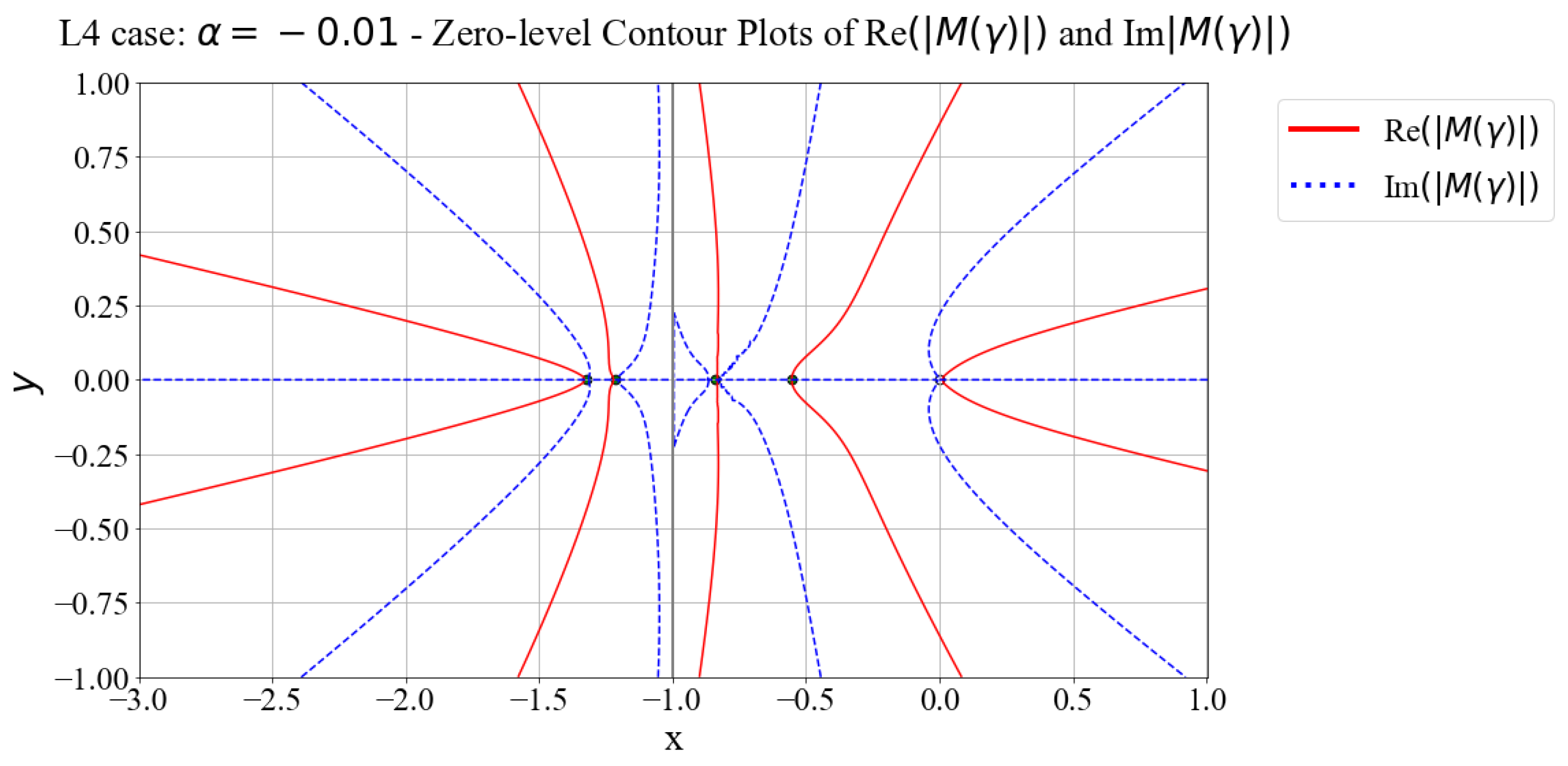
Next, we analyze an example of the L4 case. Recall that this case indicates that we have a traveling front with all real eigenvalues and a negative traveling speed c. Here, we use and .
In this case, we verify that the zeroes are the gamma values of approximately , , , , and . Since all values of such that are negative, we conclude that this particular front is linearly stable. We show this below in Figure 7.
3.5. Case L5 Analysis
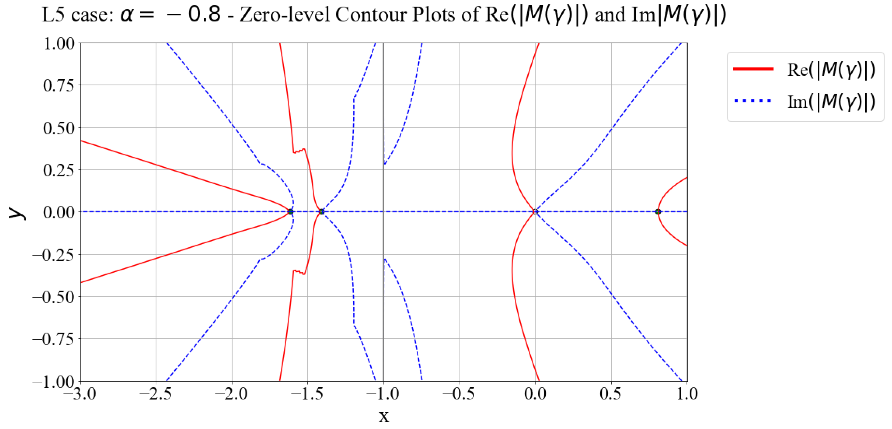
Next, we analyze an example of the L5 case. Recall that this case indicates that we have a traveling front with one conjugate pair of complex eigenvalues and three real eigenvalues and a negative traveling speed c. We take and here.
We find through computation that the zeroes are the gamma values of approximately , , , , and . In this case, we find a single positive eigenvalue, showing that this particular traveling front is unstable. We show this below in Figure 8.
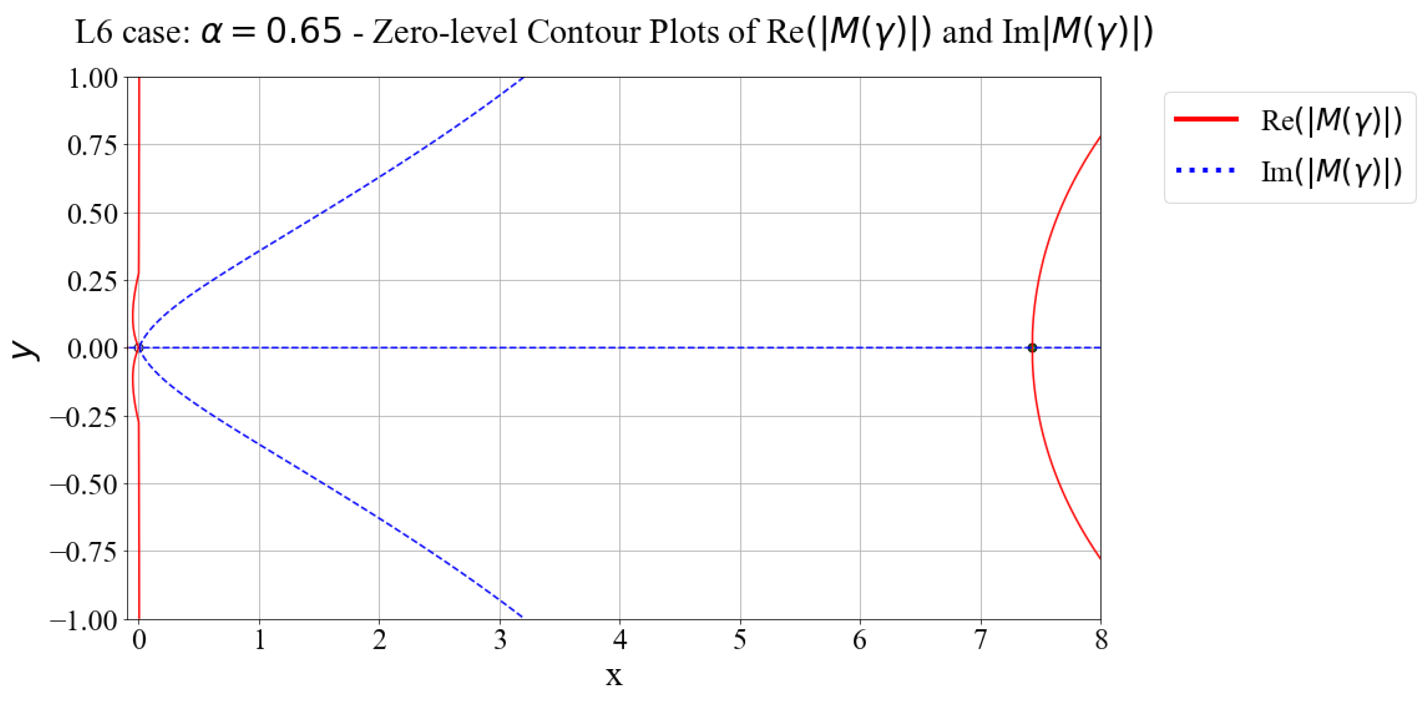
3.6. Case L6 Analysis
Finally, we analyze an example of the L6 case. Recall that this case indicates that we have a traveling front with two conjugate pairs of complex eigenvalues and one real eigenvalue and a negative traveling speed c. We use the values and . On a region entirely in the left half of the complex plane, we determine that the eigenfunction is unbounded, and therefore does not exist. However, we find a positive eigenvalue here, which makes the analysis in the left half of the complex plane unnecessary.
We compute the values of and as zeroes of the Evans function. Since we find a single positive eigenvalue, we conclude that this particular traveling front is unstable. We show this below in Figure 9.
4. Discussion
In this paper, we investigated the stability of the traveling front solutions of (4) for . We began by deriving the eigenvalue problem for the stability analysis. We did this by utilizing the method of linearization. We then looked at the equivalent ODEs and matching conditions using a differentiation approach.
We continued by investigating the possible forms for the eigenfunction by analyzing the characteristic equations of the ODEs. For the below threshold eigenfunction forms, we were able to obtain an explicit form. In the above threshold case, we had to rely on computations of the eigenvalues of the characteristic equation. Now, having the eigenfunction forms, we then showed that the determinant of the coefficient matrix, formed by the system of the eigenfunction and matching conditions, could serve as the Evans function.
At this point, we used Mathematica to calculate the zero-level curves of the real and imaginary components of the determinant, in order to find the values of such that . These values of make up the discrete spectrum, and they indicated the stability of the traveling fronts. The plots were created using Python’s matplotlib package. This allowed us to conclude that the examples we investigated in the L1 through L4 cases were linearly stable, while the L5 and L6 cases were unstable.
We did not observe any complex-valued such that in any of the cases that we studied in this paper. An interesting future investigation would be to prove that all zeroes of the Evans function are real, as seemed to be suggested here.
Author Contributions
Methodology, Y.G.; validation, Y.G.; formal analysis, D.M. and Y.G.; investigation, D.M. and Y.G.; writing—original draft, D.M.; writing—review & editing, D.M. and Y.G.; visualization, D.M. and Y.G.; supervision, Y.G. All authors have read and agreed to the published version of the manuscript.
Funding
This research received no external funding.
Institutional Review Board Statement
Not applicable.
Informed Consent Statement
Not applicable.
Data Availability Statement
Not applicable.
Acknowledgments
The authors would like to thank the reviewers of this paper for their valuable feedback.
Conflicts of Interest
The authors declare no conflict of interest.
Appendix A. Details of (16c), (16d) in Lemma (1)
Lemma A1.
Lemma (1): When analyzing the matching conditions for the equivalent ODEs of the eigenvalue Equation (6), the integral term
has the following matching conditions at :
To see (A3), we proceed with differentiation of by again utilizing the Leibniz integral rule. We find that
Now, the integral terms will again be continuous for all , but we note that for , with the threshold occurring at , that
As a result, we see that
Finally, we show (A4). We differentiate one last time, using both the Leibniz integral rule as well as the product rule, so that we obtain
After again noting that the integral terms will be continuous, we turn our attention to the term given by
By observing the limits given by
we see that
Appendix B. Examples of M(γ) Used in the Evans Function in Equation (38)
Due to the complexity and constant recalculation of the matrix used in the Evans function from Equation (38), there is not a practical way to give a general example of what this matrix looks like. We will outline and show examples of the code and procedures within Mathematica used to calculate the matrix and the relevant parameters needed in the stability analysis.
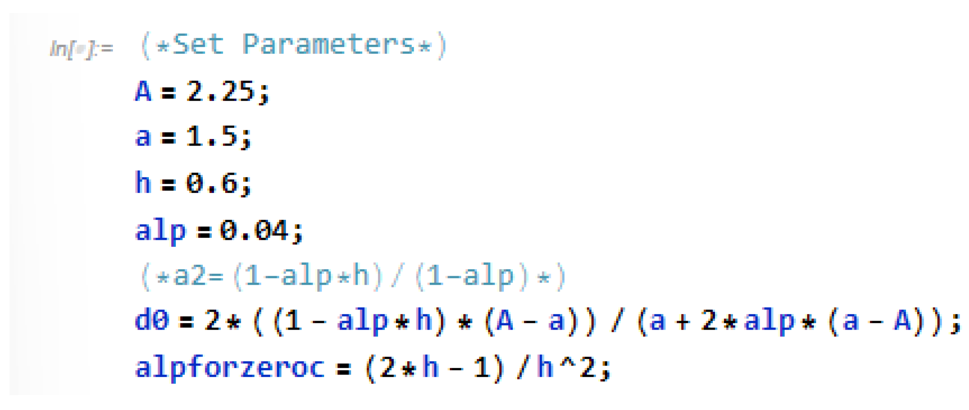
After clearing any stored variables within the software, we set the values for A, a, h, and based on the criteria of the desired front discussed in [11]. We show an example of this code in Figure A1.
Figure A1.
A sample of Mathematica code used to set parameter values.

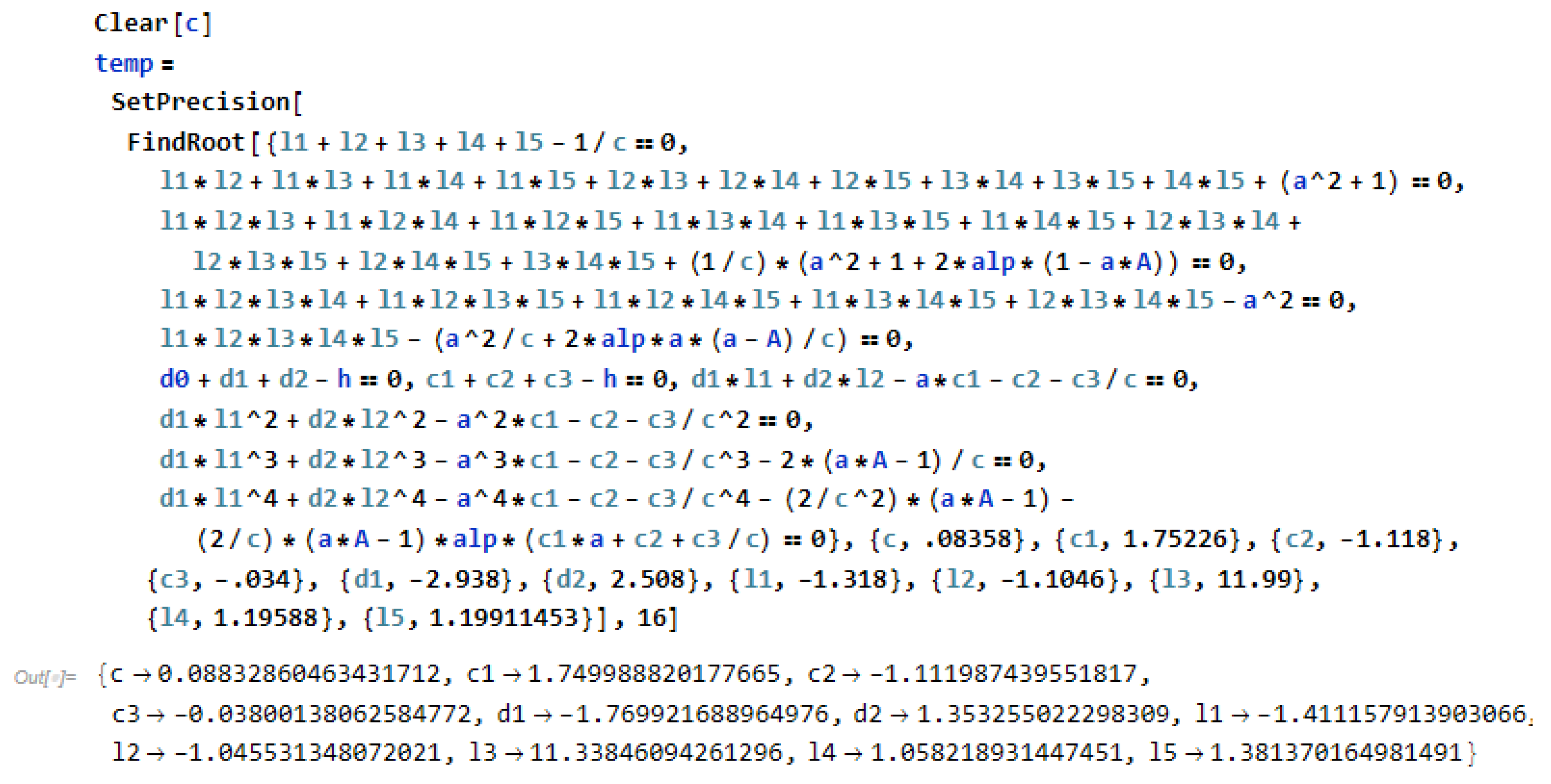
This allows us to solve a system of equations for which we obtain the front speed c, constant parameters, and eigenvalues. We show an example of this code in Figure A2.
Figure A2.
Sample of Mathematica code for solving the system of equations used to obtain traveling front parameters.
Figure A2.
Sample of Mathematica code for solving the system of equations used to obtain traveling front parameters.

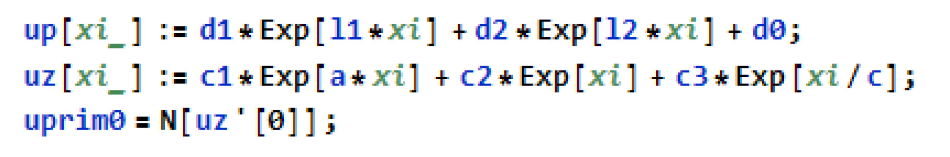
From these values, we can form the front solution, separately for above and below threshold. We also assign a variable name for for later use. We show an example of this code in Figure A3.
Figure A3.
Example of Mathematica code used for setting the above and below threshold equations for the traveling front .
Figure A3.
Example of Mathematica code used for setting the above and below threshold equations for the traveling front .

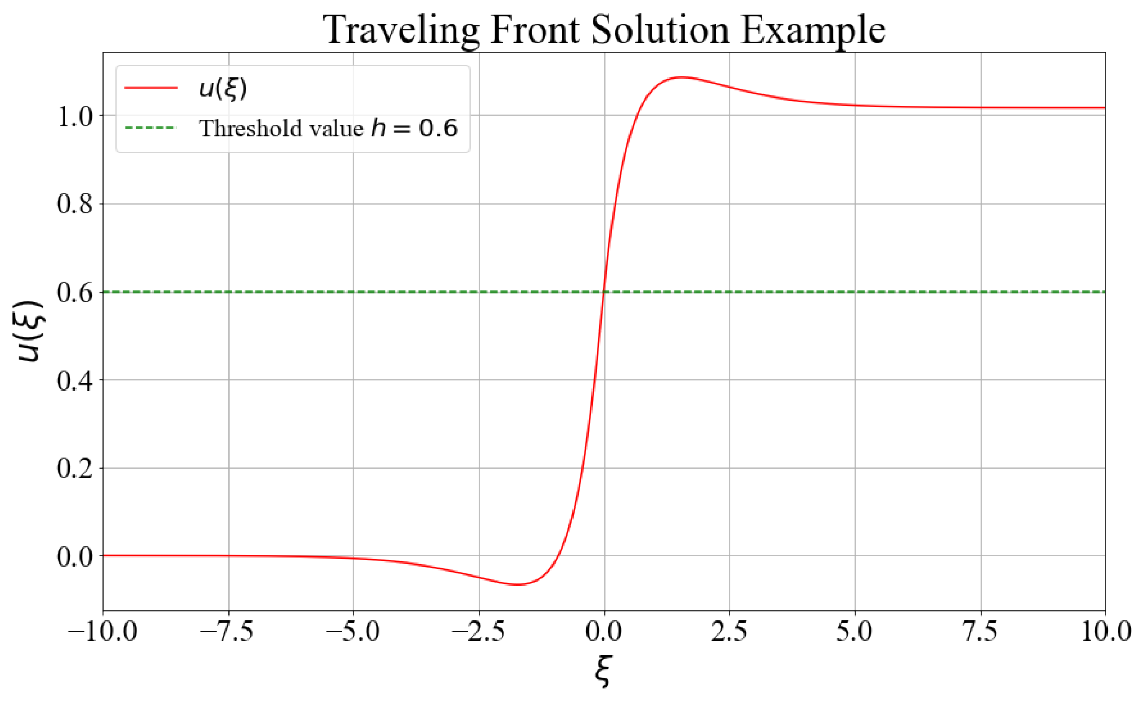
We show an example of a traveling front in Figure A4:
Figure A4.
Example of a traveling front obtained by solving the system of equations in Figure A2. Here, we solve this system in the L1 case where , , , and .
Figure A4.
Example of a traveling front obtained by solving the system of equations in Figure A2. Here, we solve this system in the L1 case where , , , and .

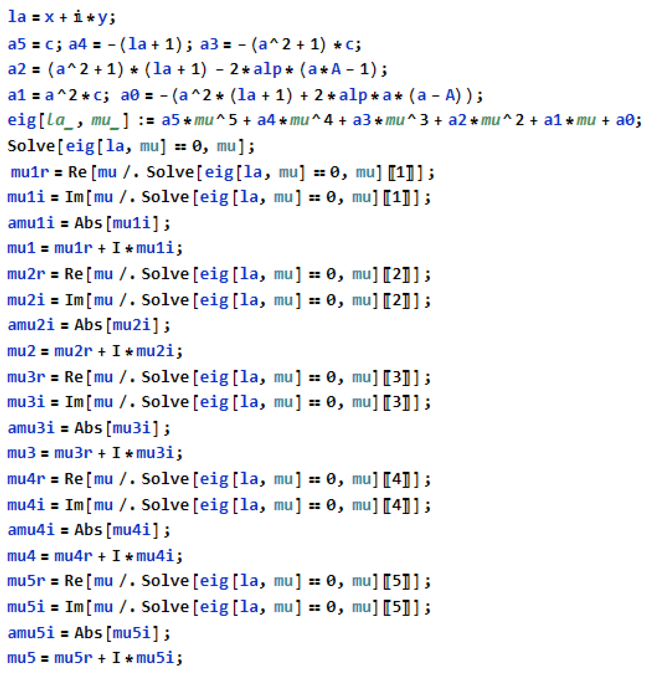
Next, after setting a desired mesh size and granularity for the calculations in the complex plane, we employ the use of a for loop to repeat the necessary calculations for each point on the complex plane. After finding the roots of the appropriate characteristic equation, (32), for the chosen value of , we assign variable names to the real part, imaginary part, and magnitude of each of the roots. We show an example of this code in Figure A5.
Figure A5.
Sample of Mathematica code for solving the characteristic Equation (32).
Figure A5.
Sample of Mathematica code for solving the characteristic Equation (32).

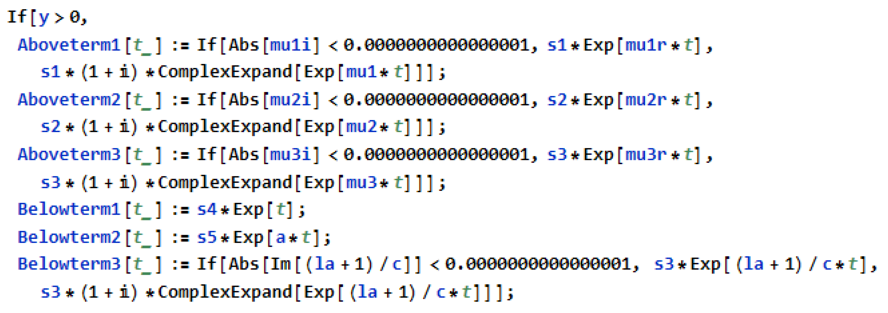
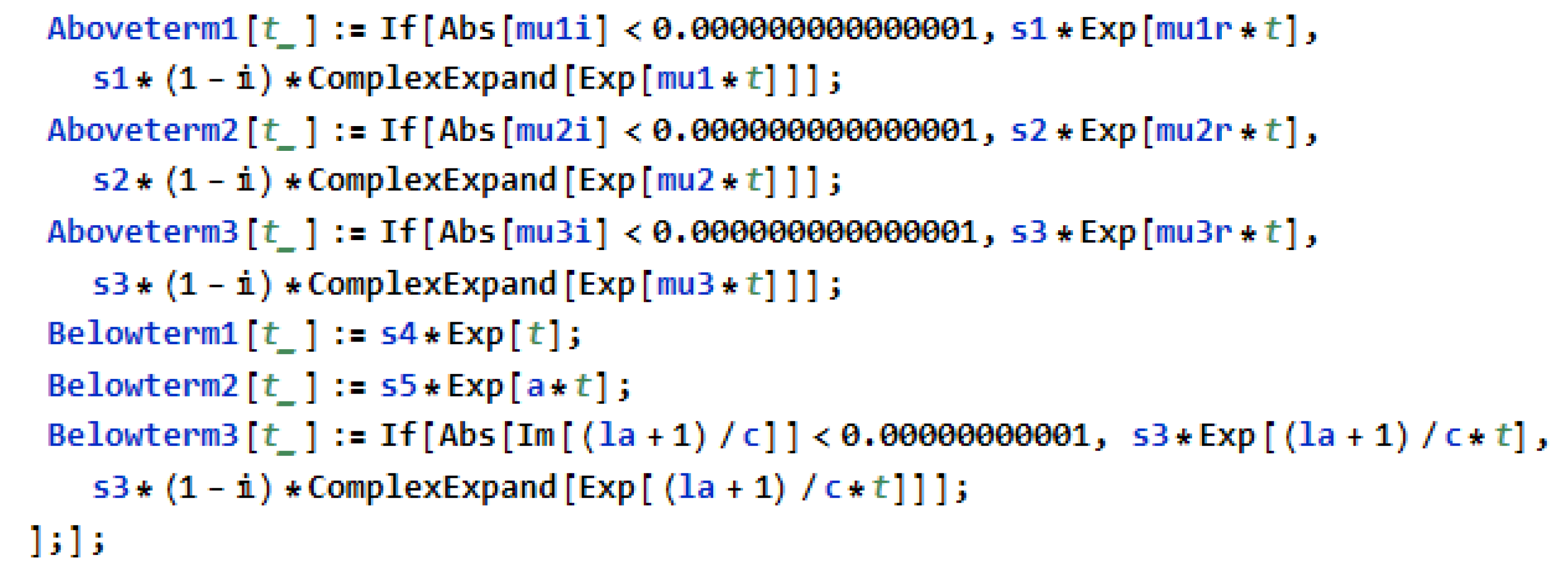
With a carefully designed series of If-Then commands, we find the expressions for each term in both the above and below threshold eigenfunctions. Depending on the current location of in the desired mesh, the roots of (32) will change in structure. The If-Then commands allowed for these changes to be accounted for in the formation of the eigenfunction, without the need to know at what precise values these changes took place. We show an example of this code in Figure A6.
Figure A6.
Sample of Mathematica code for setting the above threshold and below threshold terms of the eigenfunction when .
Figure A6.
Sample of Mathematica code for setting the above threshold and below threshold terms of the eigenfunction when .

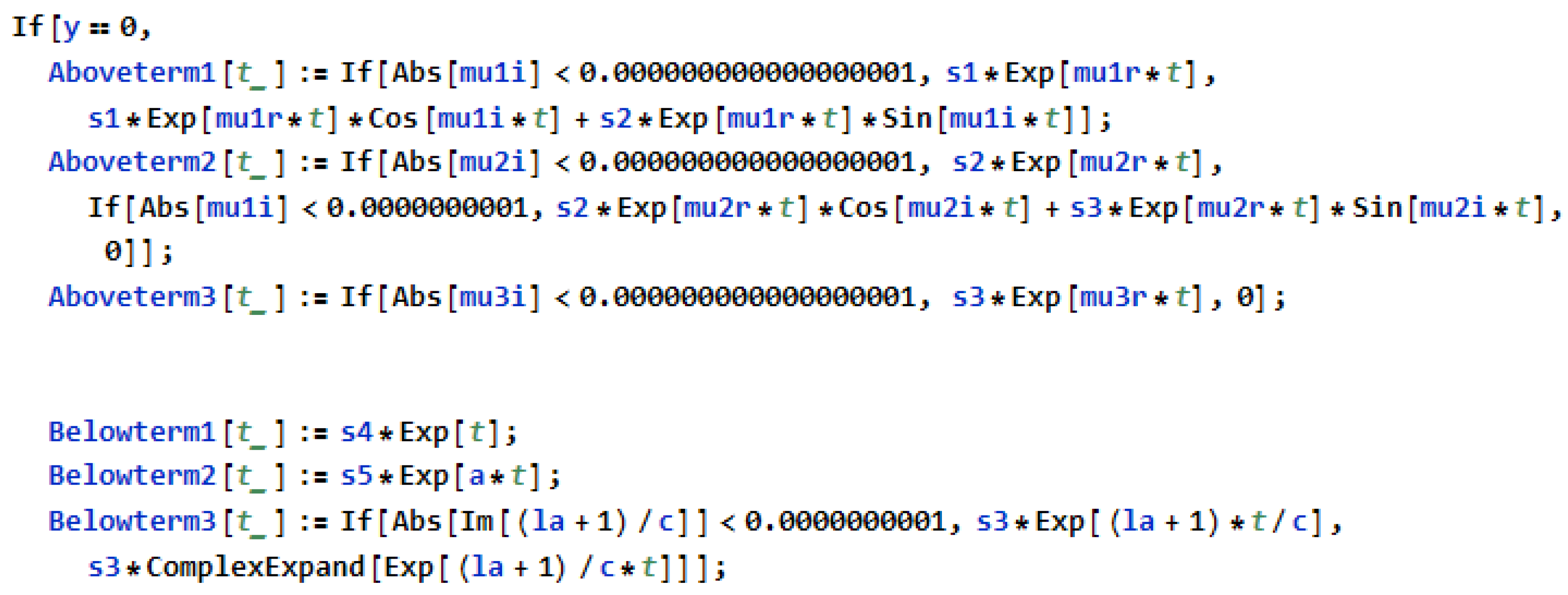
Another advantage of this setup, is that we can seamlessly integrate our more explicit knowledge of the case when . We show an example of this code in Figure A7.
Figure A7.
Sample of Mathematica code for setting the above threshold and below threshold terms of the eigenfunction when .
Figure A7.
Sample of Mathematica code for setting the above threshold and below threshold terms of the eigenfunction when .

The last section of the If-Then command handles the lower half of the complex plane. We show an example of this code in Figure A8.
Figure A8.
Sample of Mathematica code for setting the above threshold and below threshold terms of the eigenfunction when .
Figure A8.
Sample of Mathematica code for setting the above threshold and below threshold terms of the eigenfunction when .

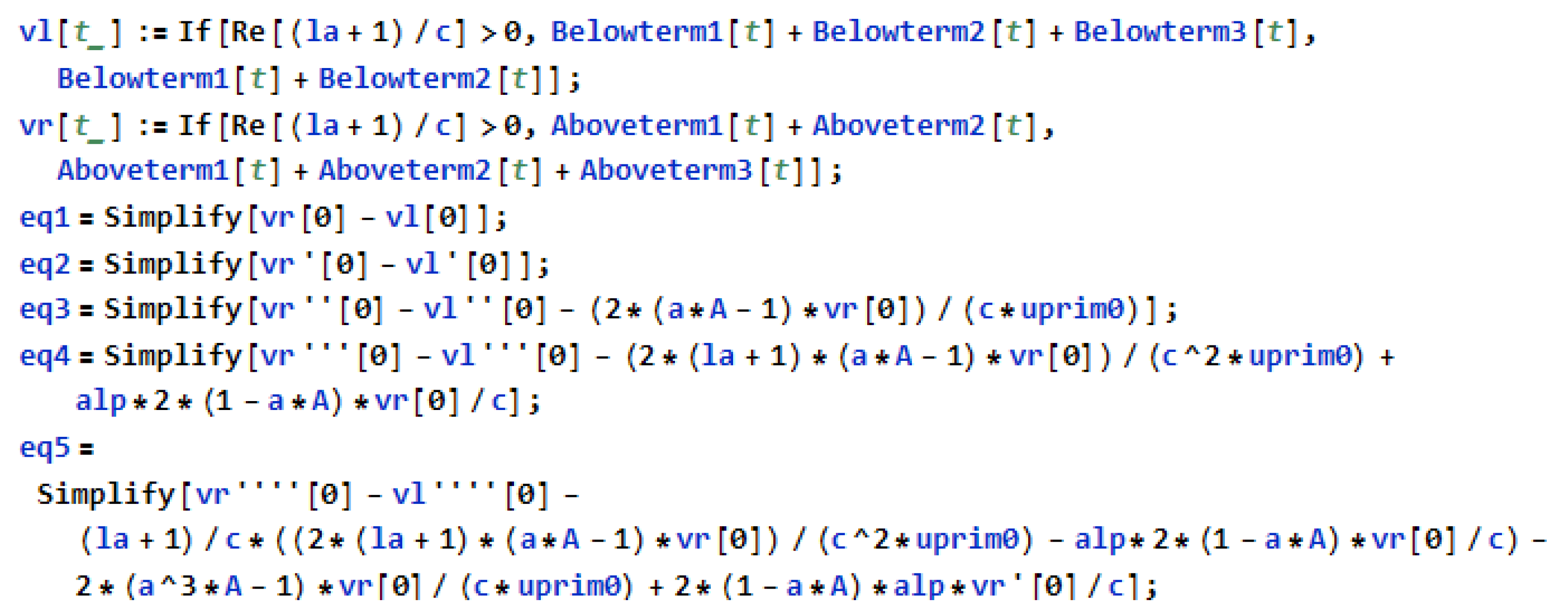
Next, we place the above and below threshold terms into the proper eigenfunction equation. Using these, we can assign variable names to the expressions that we will use to equate the matching conditions. We show an example of this code in Figure A9.
Figure A9.
Sample of Mathematica code for setting the eigenfunction and matching conditions.

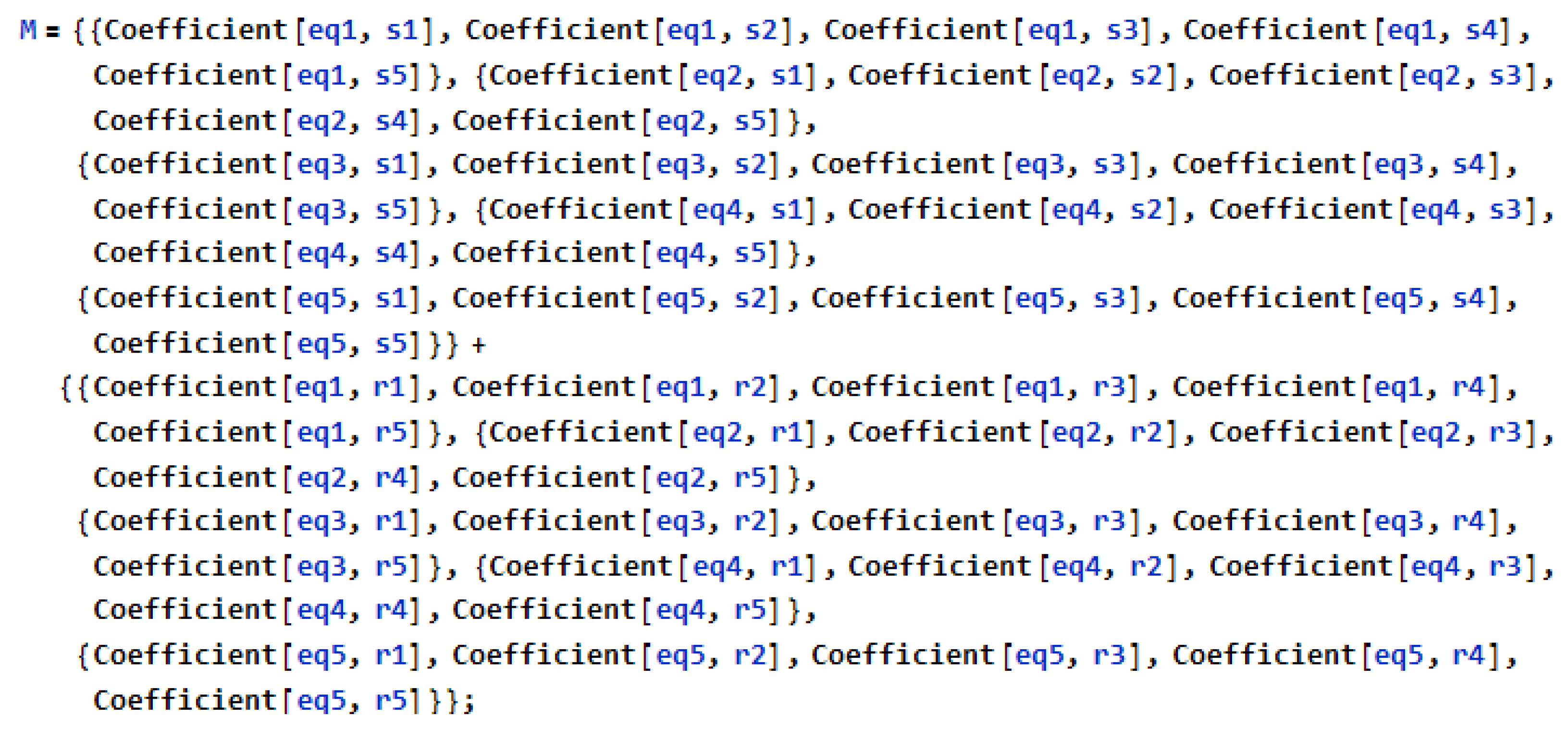
Finally, we can extract the coefficients of the matching conditions equations to give us our coefficient matrix . We show an example of this code in Figure A10.
Figure A10.
Sample of Mathematica code used to define the coefficient matrix M.

This allows us to conclude each step of the loop by calculating the determinant, with a real and imaginary component, of the matrix at each value of on the chosen mesh. This gives us a computation of the Evans function on the complex plane, allowing us to investigate the stability of the traveling fronts.
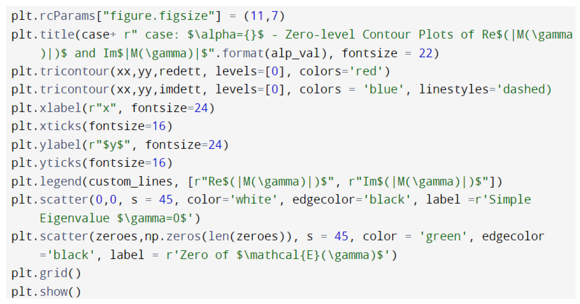
The final part of the entire procedure, after the loop is completed for our chosen mesh, is to upload the data into Python. Using the matplotlib package, we were able to plot the zero-level curves of the real and imaginary components of using a contour plot. We show an example of this code in Figure A11.
Figure A11.
Sample of Python code used to generate zero-level curves of .

We conclude by presenting a few examples of the matrix at specific values of x and y.
L1 Case, , , :
L1 Case, , , :
L4 Case, , , :
L4 Case, , , :
Appendix C. Explicit Matrix: L1 Case, α = 0, γ ∈
A closed form solution for the matrix when can be found, although this is quite messy. All calculations were performed by hand and then verified in Mathematica.
Our first step involves analyzing the simplified ODEs after the simplification of setting . As a result (7) (which remains unchanged) and (12) both become
which means that the ODE is the same on both and . In addition, due to the matching condition that , this holds on . As a result, we find that the characteristic values of this ODE are , and . In order to have a solution that converges to zero at , our solution must have one of the following forms:
and on , must have one of these following forms:
The only term that could potentially be complex-valued is the term containing . If , we can leave the term as is; if with , then we must use the previous analysis to say that
again, with . We will omit the case when in this paper. In addition, we will omit the details for the cases for when . In practice, it is extremely rare to select a value of that satisfies this equation, and the analysis would be similar in scope to that in the following subsections. We also recall the matching conditions, which will be needed in the analysis:
If and , then analyzing the matching condition at zero provides us with
and if , then we get
Analyzing the matching condition at zero for the first derivative provides us with, for
and if , then we get
For the remaining matching conditions, we must incorporate non-zero values, in order to obtain our system. In addition, we note that, since , we may use either or to evaluate this quantity. We will always use when and when for consistency.
Analyzing the matching condition at zero for the second derivative provides us with, for
and if , then we get
Analyzing the matching condition at zero for the third derivative provides us with, for
and if , then we obtain
Finally, we note the additional fact that, since , we will take when and when .
Analyzing the matching condition at zero for the fourth derivative provides us with
and if , then we have
At this point, we have the following system when :
and when :
We can now write a matrix equation of the form given in (38), specifically:
The analysis for when with follows similarly, although it becomes even messier in detail. We have chosen to omit this derivation in the paper, due to its added length, despite the similar approach we would use.
References
- Bai, L.; Huang, X.; Yang, Q.; Wu, J.Y. Spatiotemporal patterns of an evoked network oscillation in neocortical slices: Coupled local oscillators. J. Neurophysiol. 2006, 96, 2528–2538. [Google Scholar] [CrossRef] [PubMed]
- Connors, B.W.; Amitai, Y. Generation of epileptiform discharge by local circuits of neocortex. In Epilepsy: Models, Mechanisms, and Concepts; Schwartkroin, P.A., Ed.; Cambridge University Press: Cambridge, UK, 1993; pp. 388–423. [Google Scholar]
- Chervin, R.D.; Pierce, P.A.; Connors, B.W. Periodicity and directionality in the propagation of epileptiform discharges across discharges across neocortex. J. Neurophysiol. 1988, 60, 1695–1713. [Google Scholar] [CrossRef] [PubMed]
- Guo, Y.; Chow, C. Existence and stability of standing pulses in neural networks: I. Existence. SIAM J. Appl. Dyn. Syst. 2005, 4, 217–248. [Google Scholar] [CrossRef] [Green Version]
- Pfurscheller, G.; Graimann, B.; Huggins, J.E.; Levine, S.P.; Schuh, L.A. Spatiotemporal patterns of beta desynchronization and gamma synchronization in cotricographic data during self-paced movement. Clin. Neurophysiol. 2003, 114, 1226–1236. [Google Scholar] [CrossRef]
- Pfurtscheller, G.; Neuper, C.; Brunner, C.; da Silva, F.L. Beta rebound after different types of motor imagery in man. Neurosci. Lett. 2005, 378, 156–159. [Google Scholar] [CrossRef]
- Sandstede, B. Evans functions and nonlinear stability of travelling waves in neuronal network models. Int. J. Bifurc. Chaos 2007, 17, 2693–2704. [Google Scholar] [CrossRef]
- Amari, S. Dynamics of Pattern Formation in Lateral-Inhibition Type Neural Fields. Biol. Cybern. 1977, 27, 77–87. [Google Scholar] [CrossRef]
- Ermentrout, G.B.; McLeod, B.J. Existence and uniqueness of traveling waves for a neural network. Proc. R. Soc. Edinb. Sect. A Math. 1993, 123A, 461–478. [Google Scholar] [CrossRef]
- Zhang, L. On stability of traveling wave solutions in synaptically coupled neuronal networks. Differ. Integral Equ. 2003, 16, 513–536. [Google Scholar] [CrossRef]
- Guo, Y. Existence and Stability of Traveling Fronts in a Lateral Inhibition Neural Network. SIAM J. Appl. Dyn. Syst. 2012, 11, 1543–1582. [Google Scholar] [CrossRef] [Green Version]
- Coombes, S.; Owen, M.R. Evans functions for integral neural field equations with Heaviside firing rate function. SIAM J. Appl. Dyn. Syst. 2004, 3, 574–600. [Google Scholar] [CrossRef] [Green Version]
- Coombes, S.; Schmidt, H.; Bojak, I. Interface dynamics in planar neural field models. J. Math. Neurosci. 2012, 2, 1–27. [Google Scholar] [CrossRef] [PubMed] [Green Version]
- Coombes, S.; Thul, R.; Laing, C. Neural Field Models with Threshold Noise. J. Math. Neurosci. 2016, 6, 3. [Google Scholar]
- Coombes, S.; Avitabile, D.; Gokce, A. The Dynamics of Neural Fields on Bounded Domains: An Interface Approach for Dirichlet Boundary Conditions. J. Math. Neurosci. 2017, 7, 12. [Google Scholar]
- Cook, B.; Peterson, A.; Woldman, W.; Terry, J. Neural Field Models: A mathematical overview and unifying framework. Math Neuro. Appl. 2022, 2, 1–67. [Google Scholar] [CrossRef]
- Qin, Z.; Fu, Q.; Jin, D.; Peng, J. A Looming Perception Model Based on Dynamic Neural Field. 2022. Available online: https://ssrn.com/abstract=4248213 (accessed on 28 January 2023).
- González-Ramírez, L.R. On the existence of traveling fronts in the fractional-order Amari neural field model. Commun. Nonlinear Sci. Numer. Simul. 2023, 116, 106790. [Google Scholar] [CrossRef]
- Laing, C.R.; Troy, w.C.; Gutkin, B.; Ermentrout, G.B. Multiple Bumps in a Neuronal Model of Working Memory. SIAM J. Appl. Math. 2002, 63, 62–97. [Google Scholar] [CrossRef]
- Laing, C.R.; Troy, W.C. Two-bump Solutions of Amari-type Models of Neuronal Pattern Formation. Phys. D Nonlinear Phenom. 2003, 178, 190–218. [Google Scholar] [CrossRef]
- Janson, S. Resultant and Discriminant of Polynomials. 2010. Available online: http://www2.math.uu.se/~svante/papers/sjN5 (accessed on 19 March 2020).
- Evans, J.W. Nerve axon equations, I: Linear approximations. Indiana Univ. Math. J. 1972, 21, 877–955. [Google Scholar] [CrossRef]
- Evans, J.W. Nerve axon equations, II: Stability at rest. Indiana Univ. Math. J. 1972, 22, 75–90. [Google Scholar] [CrossRef]
- Evans, J.W. Nerve axon equations, III: Stability of the nerve impulse. Indiana Univ. Math. J. 1972, 22, 577–594. [Google Scholar] [CrossRef]
- Evans, J.W. Nerve axon equations, IV: The stable and unstable impulse. Indiana Univ. Math. J. 1975, 24, 1169–1190. [Google Scholar] [CrossRef]
- Zhang, L. Existence, uniqueness and exponential stability of traveling wave solutions of some integral differential equations arising from neuronal networks. J. Differ. Equ. 2004, 197, 162–196. [Google Scholar] [CrossRef] [Green Version]
Figure 1.
Coupling function example.

Figure 2.
Gain function example.

Figure 3.
L1 Case—plot of complex Evans function zero-level contours. Traveling front has all real eigenvalues and traveling speed c. Relevant parameters are , , and .
Figure 3.
L1 Case—plot of complex Evans function zero-level contours. Traveling front has all real eigenvalues and traveling speed c. Relevant parameters are , , and .

Figure 4.
L1 Case—plot of complex Evans function zero-level contours. Traveling front has all real eigenvalues and traveling speed c. Relevant parameters are , , and .
Figure 4.
L1 Case—plot of complex Evans function zero-level contours. Traveling front has all real eigenvalues and traveling speed c. Relevant parameters are , , and .

Figure 5.
L2 Case—plot of complex Evans function zero-level contours. Traveling front has all real eigenvalues and traveling speed c. Relevant parameters are , , and .
Figure 5.
L2 Case—plot of complex Evans function zero-level contours. Traveling front has all real eigenvalues and traveling speed c. Relevant parameters are , , and .

Figure 6.
L3 Case—plot of complex Evans function zero-level contours. Traveling front has all real eigenvalues and traveling speed c. Relevant parameters are , , and .
Figure 6.
L3 Case—plot of complex Evans function zero-level contours. Traveling front has all real eigenvalues and traveling speed c. Relevant parameters are , , and .

Figure 7.
L4 Case—plot of complex Evans function zero-level contours. Traveling front has all real eigenvalues and a traveling speed c. Relevant parameters are , , and .
Figure 7.
L4 Case—plot of complex Evans function zero-level contours. Traveling front has all real eigenvalues and a traveling speed c. Relevant parameters are , , and .

Figure 8.
L5 Case—Plot of complex Evans function zero-level contours. Traveling front has all real eigenvalues and traveling speed c. Relevant parameters are , , and .
Figure 8.
L5 Case—Plot of complex Evans function zero-level contours. Traveling front has all real eigenvalues and traveling speed c. Relevant parameters are , , and .

Figure 9.
L6 Case—plot of complex Evans function zero-level contours. Traveling front has all real eigenvalues and traveling speed c. Relevant parameters are , , and .
Figure 9.
L6 Case—plot of complex Evans function zero-level contours. Traveling front has all real eigenvalues and traveling speed c. Relevant parameters are , , and .

Disclaimer/Publisher’s Note: The statements, opinions and data contained in all publications are solely those of the individual author(s) and contributor(s) and not of MDPI and/or the editor(s). MDPI and/or the editor(s) disclaim responsibility for any injury to people or property resulting from any ideas, methods, instructions or products referred to in the content. |
© 2023 by the authors. Licensee MDPI, Basel, Switzerland. This article is an open access article distributed under the terms and conditions of the Creative Commons Attribution (CC BY) license (https://creativecommons.org/licenses/by/4.0/).
Share and Cite
MDPI and ACS Style
Macaluso, D.; Guo, Y. Stability of Traveling Fronts in a Neural Field Model. Mathematics 2023, 11, 2202. https://doi.org/10.3390/math11092202
AMA Style
Macaluso D, Guo Y. Stability of Traveling Fronts in a Neural Field Model. Mathematics. 2023; 11(9):2202. https://doi.org/10.3390/math11092202
Chicago/Turabian StyleMacaluso, Dominick, and Yixin Guo. 2023. "Stability of Traveling Fronts in a Neural Field Model" Mathematics 11, no. 9: 2202. https://doi.org/10.3390/math11092202
Note that from the first issue of 2016, this journal uses article numbers instead of page numbers. See further details here.