Article

Partial Slip Effects for Thermally Radiative Convective Nanofluid Flow

by
Remus-Daniel Ene
1,†,
Nicolina Pop
2,*,† and
Rodica Badarau
3,†
1
Department of Mathematics, Politehnica University of Timisoara, 300006 Timisoara, Romania
2
Department of Physical Foundations of Engineering, Politehnica University of Timisoara, 2 Vasile Parvan Blvd., 300223 Timisoara, Romania
3
Department of Mechanical Machines, Equipment and Transportation, Politehnica University of Timisoara, 1 Mihai Viteazul Blvd., 300222 Timisoara, Romania
*
Author to whom correspondence should be addressed.
These authors contributed equally to this work.
Mathematics 2023, 11(9), 2199; https://doi.org/10.3390/math11092199
Submission received: 30 March 2023 / Revised: 20 April 2023 / Accepted: 5 May 2023 / Published: 6 May 2023
(This article belongs to the Special Issue Nonlinear Vibration Theory and Mechanical Dynamics)

Abstract

:
The partial slip effects for radiative convective nanofluid flow over a stretching sheet in porous medium are analytically explored in this work. The Navier–Stokes equations, the momentum and the energy equations are converted into a set of non-linear ODEs by the similarity transformation. Using the modified optimal homotopy asymptotic method (OHAM), the resulting non-linear ODEs are analytically approximately solved. The impact of various parameters, such as: the velocity exponential factor n, the wall thickness parameter γ , the dimensionless velocity slip parameter δ 1 , the Prandtl number P r , the radiation parameter R, and the dimensionless temperature jump parameter δ 2 , on the behaviour of the mass and heat transfer is presented. The influence of these parameters is tabular and graphically presented. An excellent agreement between the approximate analytical solution and the corresponding numerical solution is highlighted. The results obtained confirm that modified OHAM is a useful and competitive mathematical tool to explore a large class of non-linear problems with applications in various fields of science and engineering.

1. Introduction

The study of the nanofluid flow has gained considerable attention in recent decades due to its importance in many industrial applications, especially in nanotechnology.
Nanofluids are fluids that contain nanoparticles with superior thermal conductivity properties (silver, copper, iron, carbon nanotubes, CuO, SiO, etc.) in suspension. The aim of using nanofluids is to significantly improve heat transfer by increasing the thermal conductivity of base fluids (ethylene glycol, water, motor oil, acetone, etc.). Solving the equations that characterize nanofluids is important because they govern a very important class of common physical processes. Computational techniques and new approximation methods have made it possible to solve these equations with increasing accuracy, confirming experimental results in broad engineering fields such as: industrial manufacturing processes in the industry of materials with plastic behaviour (extrusion of polymers, spinning of polymer fibres, fibre spinning and drawing plastic films), metal casting, hot rolling, metal spinning, paper manufacture, glass blowing, etc. The equations are also used to model physical phenomena related to fluid flow in the boundary layer, flow processes in porous media with applications in wastewater treatment systems and soil de-pollution in drying beds, in the mining industry.
Many researchers have carried out both experimental and theoretical approaches concerning the boundary layer and heat transfer over a stretching sheet.
In recent years several analytical methods for solving the non-linear differential problem have been used to model the heat and mass transfer in a viscous fluid/nanofluid flow [1,2,3,4,5,6,7] were applied.
Vishalakshi et al. [1] obtained the closed-form exact solutions of highly non-linear differential equations of the Walters’ liquid B flow. The mass transfer of a chemically reactive species and the flow of MHD over a stretching plate subjected to an inclined magnetic field were examined by Maranna et al. [2]. Sarma et al. [3] explored the exact solution to the problem of a free convective, radiative, viscous, chemically reacting, heat absorbing, incompressible, and unsteady MHD flow using the Laplace transformation technique.
Mahabaleshwar et al. [4] and Akhtar et al. [5] developed novel mathematical techniques to build analytical solutions to non-Newtonian Casson fluid flow.
The velocity and thermal slips of MHD boundary layer flow of Williamson nanofluid was numerically discussed by Reddy et al. [8]. On the other hand, some methods have given numerical solutions. Abbas et al. [9] proposed a model in terms of partial differential equations to study the influence of the Darcy–Forchheimer relation on third-grade fluid flow and heat transfer taking into account the applied magnetic field, Joule heating, thermal diffusion, viscous dissipation, and diffusion-thermo effects. Elbashbeshy et al. [10] analysed the boundary layer flow of a nanofluid containing gyrotactic microorganisms over a vertical stretching surface. Nuwairan et al. [11] explored a model governing a Maxwell nanofluid flow with the effect of activation energy with addition of heat generation/absorption and thermal radiation. Abbas et al. [12] examined the hybrid nanofluid flow past a permeable curved surface with non-linear stretching with injection/suction. Hossein et al. [13] examined the effects of progressive developments in cross-section design, the fuel cell structure, the output current densities and the flooding phenomenon using the finite volume method, and so on [14,15,16,17,18,19,20,21,22,23,24,25,26,27,28,29,30,31,32,33,34,35,36,37,38].
In the present work, the modified optimal homotopy asymptotic method (OHAM [39,40,41,42,43,44,45] is used to obtain the effective and accurate analytic approximate solutions. This procedure does not depend on small or large parameters and gives us a simple way to optimally control the convergence of approximate solutions using a single iteration.
Our paper is organized as: The introduction is followed by a brief description of the theoretical approach including the steps of the modified OHAM technique in Section 2. Section 3 presents the heat and mass transfer problem by the modified OHAM. The results and some interesting discussions about the effects of non-linear stretching on the flow and heat transfer characteristics are highlighted in Section 4. Conclusions are presented the last section of this paper.

2. Theoretical Approach

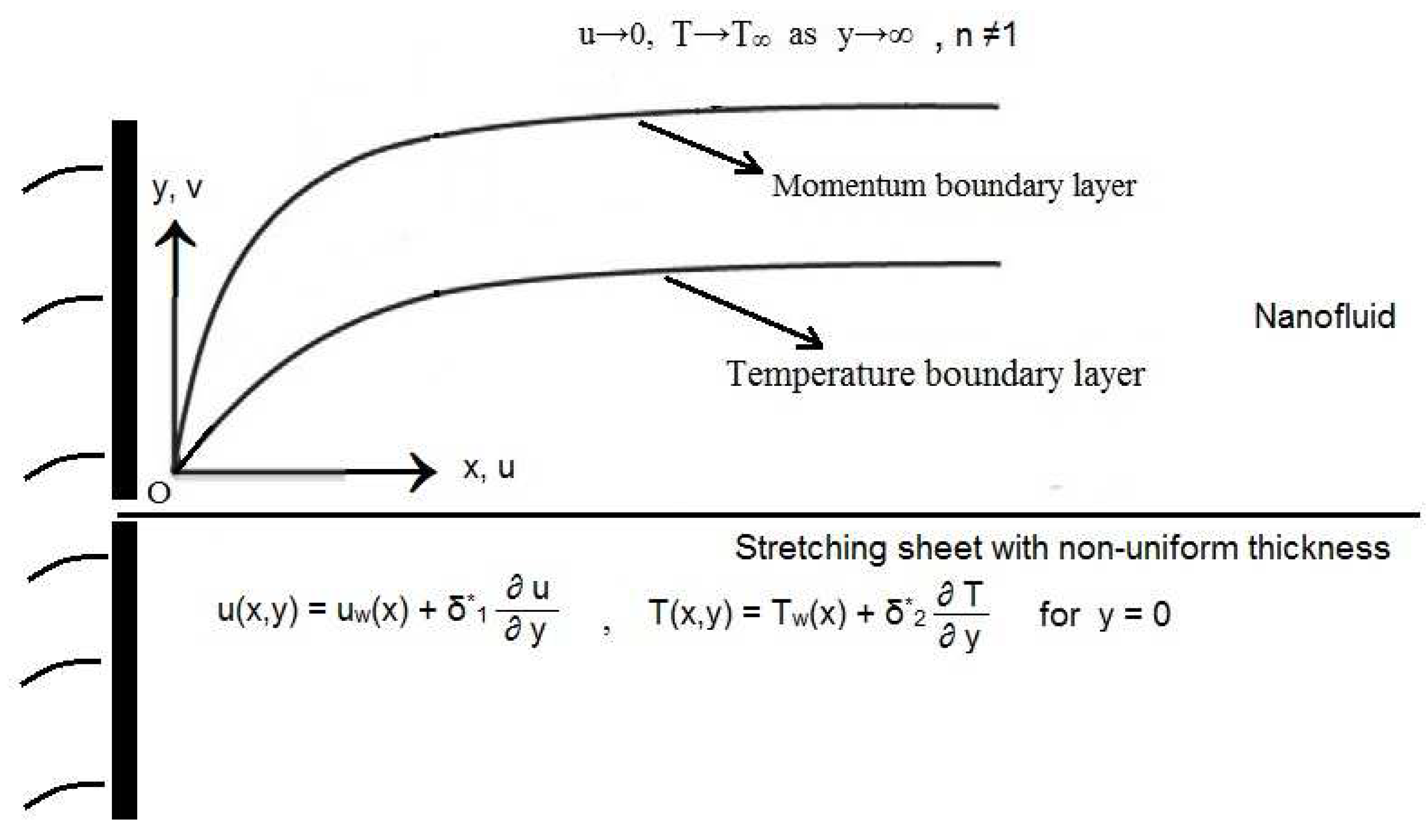
2.1. Equations of Motion

The Navier slip conditions are considered for a steady two-dimensional, incompressible, laminar, hydrodynamic flow of a nano fluid over a stretching sheet with non-uniform thickness in porous medium. The sheet is along the x-axis direction and y-axis is normal to it. A non-uniform permeability K ( x ) = k 0 ( x + a ) 1 n , n 1 along with the thermal radiation effect is taken into account. Viscous dissipation effect is neglected in this study. It is assumed that the sheet is stretched with the velocity u w ( x ) = u 0 ( x + a ) n , n 1 and the wall temperature T w ( x ) = T + T 0 ( x + a ) ( 1 n ) / 2 , n 1 . Since the sheet is non-uniform it is assumed that y = A ( x + a ) ( 1 n ) / 2 , n 1 , where A is the coefficient related to stretching sheet and chosen as a small constant to avoid the external pressure. At n = 1 the problem refers flat stretching sheet case.
The physical model is schematically presented in Figure 1.
As per the above assumptions the governing boundary layer equations are given as follows [46,47]:
u x + v y = 0 ,
u u x + v s . u y = ν f 2 u y 2 ,
u T x + v s . T y = α 2 T y 2 1 ( ρ c p ) f · q r y .
The boundary conditions are as follows:
u ( x , y ) = u w ( x ) + δ 1 u y , v ( x , y ) = 0 , T ( x , y ) = T w ( x ) + δ 2 T y at y = 0 , u ( x , y ) 0 , T ( x , y ) T , n 1 , at y ,
where u and v are the velocity components along the x and y directions, respectively, ν f is the kinematic viscosity, T is the temperature of the fluid, k is the thermal conductivity, α is the thermal diffusivity of the nanofluid, ( ρ c p ) f is the specific heat capacitance, δ 1 is the dimensional velocity slip parameter and δ 2 is dimensional temperature jump parameter, these are given by δ 1 = 2 b b ξ 1 ( x + a ) ( 1 n ) / 2 , δ 2 = 2 c c ξ 2 ( x + a ) ( 1 n ) / 2 , ξ 2 = 2 λ λ + 1 ξ 1 P r . Here ξ 1 and ξ 2 are mean free paths and λ is the ratio of specific heats, b and c, respectively, indicating Maxwell’s reflection coefficient and thermal accommodation coefficient.
The radiative heat flux q r under the Rosseland approximation has the form [48]:
q r = 4 σ 3 k · T 4 y ,
where σ is the Stefan–Boltzmann constant and k is the mean absorption coefficient. The temperature differences within the flow are assumed to be sufficiently small such that T 4 may be expressed as a linear function of temperature. Expanding T 4 using a Taylor series and neglecting higher-order terms yields
T 4 4 T 3 T 3 T 4 .
The governing Equations are converted into a set of non-linear ordinary differential equations by means of the following similarity transformation [46,47]:
ψ ( x , y ) = 2 ν f u 0 n + 1 1 / 2 · ( x + a ) ( n + 1 ) / 2 · f ( η ) , η = ( n + 1 ) u 0 2 ν f 1 / 2 · ( x + a ) ( n 1 ) / 2 · y , n 1 , θ ( η ) = T T T w ( x ) T ,
where ψ ( x , y ) is a stream function which satisfies the continuity Equation (1) with
u = ψ ( x , y ) y and v s . = ψ ( x , y ) x .
Taking into account of Equations (5)–(8), Equations (2) and (3) become:
f + f f 2 n n + 1 ( f ) 2 = 0 ,
1 P r 1 + 4 3 R θ 1 n 1 + n f θ + f θ = 0 ,
with the transformed boundary conditions
f ( 0 ) = γ 1 n 1 + n [ 1 + δ 1 · f ( 0 ) ] , f ( 0 ) = 1 + δ 1 · f ( 0 ) , θ ( 0 ) = 1 + δ 2 · θ ( 0 ) , f ( ) 0 , θ ( ) 0 , n 1 ,
where γ = A · ( n + 1 ) u 0 2 ν f 1 / 2 , δ 1 = 2 b b · ξ 1 · ( n + 1 ) u 0 2 ν f 1 / 2 , δ 2 = 2 c c · ξ 2 · ( n + 1 ) u 0 2 ν f 1 / 2 , the prime indicates the differentiation with respect to η , P r = ν f / α is the Prandtl number, R = 4 σ T 3 k k is the radiation parameter, n is the velocity power index parameter, γ is the wall thickness parameter, δ 1 is the dimensionless velocity slip parameter, and δ 2 is the dimensionless temperature jump parameter.
For engineering the shear stress coefficient or friction factor ( C f ) and local Nusselt number ( N u x ) are given by
R e x 0.5 C f = 2 n + 1 2 0.5 f ( 0 ) ,
and
R e x 0.5 N u x = n + 1 2 0.5 θ ( 0 ) ,
where R e x = u w ( x + a ) ν f is the local Reynolds number.

2.2. Steps of the Modified Optimal Homotopy Asymptotic Method (OHAM)

The OHAM technique [39] has the following steps:
(i) The non-linear differential equation has the general form:
L F ( η ) + N F ( η ) = 0 ,
with the boundary/initial conditions
B F ( η ) , d F ( η ) d η = 0 ,
where L F ( η ) and N F ( η ) describe the linear part and the non-linear part, respectively, and B is an operator describing the boundary conditions, while F ( η ) is the unknown smooth function.
(ii) The homotopic relation is given by:
H L F ( η , p ) , H ( η , C i ) , N F ( η , p ) = L F 0 ( η ) + G ( η ) + p L F 1 ( η , C i ) H ( η , C i ) N F 0 ( η ) ,
where G ( η ) is a known function, p [ 0 , 1 ] is the embedding parameter and H ( η , C i ) 0 is an auxiliary convergence-control function depending on the variable η , the parameters C 1 , C 2 , …, C s , and choosing the unknown function F ( η ) in the form:
F ( η , p ) = F 0 ( η ) + p F 1 ( η , C i ) ,
and by equating the coefficients of p 0 and p 1 , respectively, yields:
the zeroth-order deformation problem
L F 0 ( η ) + G ( η ) = 0 , B F 0 ( η ) , d F 0 ( η ) d η = 0 ,
the first-order deformation problem
L F 1 ( η , C i ) = H ( η , C i ) N F 0 ( η ) , B F 1 ( η , C i ) , d F 1 ( η , C i ) d η = 0 , i = 1 , 2 , , s .
(iii) The initial approximation F 0 ( η ) can be obtained by solving the linear Equation (16).
(iv) In order to compute F 1 ( η , C i ) by Equation (17), for the non-linear operator N was chosen general form
N F 0 ( η ) = i = 1 n h i ( η ) g i ( η ) ,
where n is a positive integer, and h i ( η ) and g i ( η ) are known elementary functions that depend on F 0 ( η ) and N .
The computation of the first approximation F 1 ( η , C i ) leads to:
F 1 ( η , C i ) = i = 1 m H i ( η , h j ( η ) , C j ) g i ( η ) , j = 1 , , s ,
or
F 1 ( η , C i ) = i = 1 m H i ( η , g j ( η ) , C j ) h i ( η ) , j = 1 , , s , B F 1 ( η , C i ) , d F 1 ( η , C i ) d η = 0 .
The above expressions of H i ( η , h j ( η ) , C j ) contain linear combinations of the elementary functions h j , j = 1 , , s and the parameters C j , j = 1 , , s . The summation limit m is an arbitrary positive integer.
(v) The first-order analytical approximate solutions of Equations (12) and (13), taking into account Equation (15), could be written as:
F ¯ ( η , C i ) = F ( η , 1 ) = F 0 ( η ) + F 1 ( η , C i ) .
The convergence-control parameters C 1 , C 2 , …, C s can be optimally identified by various methods, such as: the Kantorowich method, the collocation method, the Galerkin method, the least square method, or the weighted residual method.
Therefore, in this case we construct an analytic approximate solution using the modified optimal homotopy asymptotic method (OHAM).

3. Heat and Mass Transfer Problem by the Modified OHAM

OHAM procedure will be apply in order to obtain approximate solutions to Equations (9) and (10) with the initial/boundary conditions in Equation (11).
For this purpose, for the non-linear Equation (9), we choose the linear operator of the form:
L f η = f ( η ) K 1 2 f ( η ) + G ( η ) ,
where the given arbitrary function G ( η ) = a e K 2 η + c 1 e K 0 η + c 2 e 2 K 0 η + c 3 e 3 K 0 η and K 0 , K 1 , K 2 , a, c 1 , c 2 , c 3 are some unknown positive parameters to be determined later.
The initial approximation f 0 ( η ) can be obtained from the following problem:
f 0 ( η ) K 1 2 f 0 ( η ) + G ( η ) = 0 , f 0 ( 0 ) = γ · 1 n 1 + n · f 0 ( 0 ) , f 0 ( 0 ) = 1 + δ 1 f 0 ( 0 ) , f 0 ( ) = 0 ,
with the solution:
f 0 ( η ) = b 0 + b 1 e K 1 η + b 2 e K 2 η + d 1 e K 0 η + d 2 e 2 K 0 η + d 3 e 3 K 0 η ,
where
d 1 = c 1 K 0 3 K 0 K 1 2 , d 2 = c 2 8 K 0 3 2 K 0 K 1 2 , d 3 = c 3 27 K 0 3 3 K 0 K 1 2 , b 2 = a K 2 3 K 2 K 1 2 ,
b 1 = 1 K 1 2 + K 1 · 1 + a ( 1 + K 2 ) K 2 2 K 1 2 + c 1 ( 1 + K 0 ) K 0 2 K 1 2 + c 2 ( 1 + 2 K 0 ) 4 K 0 2 K 1 2 + c 3 ( 1 + 3 K 0 ) 9 K 0 2 K 1 2 ,
b 0 = γ 1 n 1 + n · b 1 K 1 b 2 K 2 d 1 K 0 2 d 2 K 0 3 d 3 K 0 b 1 b 2 d 1 d 2 d 3 .
The non-linear operator N f ( η ) , corresponding to the non-linear differential Equation (9), is defined by:
N f η = f f 2 n n + 1 ( f ) 2 + K 1 2 f .
For the initial approximation f 0 ( η ) given by Equation (24), the non-linear operator Equation (25) becomes:
N f 0 ( η ) = f 0 f 0 2 n n + 1 ( f 0 ) 2 + K 1 2 f 0 = = m 1 e K 0 η + m 2 e 2 K 0 η + m 3 e 3 K 0 η + m 4 e 4 K 0 η + m 5 e 5 K 0 η + m 6 e 6 K 0 η + m 7 e K 1 η + + m 8 e 2 K 1 η + m 9 e K 2 η + m 10 e 2 K 2 η + m 11 e ( K 1 + K 0 ) η + m 12 e ( K 1 + 2 K 0 ) η + m 13 e ( K 1 + 3 K 0 ) η + + m 14 e ( K 2 + K 0 ) η + m 15 e ( K 2 + 2 K 0 ) η + m 16 e ( K 2 + 3 K 0 ) η + m 17 e ( K 1 + K 2 ) η ,
where
m 1 = b 0 d 1 K 0 2 d 1 K 0 K 1 2 , m 2 = d 1 2 K 0 2 + 4 b 0 d 2 K 0 2 d 1 2 K 0 2 · 2 n n + 1 2 d 2 K 0 K 1 2 ,
m 3 = 5 d 1 d 2 K 0 2 + 9 b 0 d 3 K 0 2 4 d 1 d 2 K 0 2 · 2 n n + 1 3 d 3 K 0 K 1 2 ,
m 4 = 4 d 2 2 K 0 2 + 10 d 1 d 3 K 0 2 4 d 2 2 K 0 2 · 2 n n + 1 6 d 1 d 3 K 0 2 · 2 n n + 1 ,
m 5 = 13 d 2 d 3 K 0 2 12 d 2 d 3 K 0 2 · 2 n n + 1 , m 6 = 9 d 3 2 K 0 2 9 d 3 2 K 0 2 · 2 n n + 1 ,
m 7 = b 0 b 1 K 1 2 b 1 K 1 3 , m 8 = b 1 2 K 1 2 b 1 2 K 1 2 · 2 n n + 1 ,
m 9 = b 0 b 2 K 2 2 b 2 K 2 K 1 2 , m 10 = b 2 2 K 2 2 b 2 2 K 2 2 · 2 n n + 1 ,
m 11 = b 1 d 1 K 0 2 + b 1 d 1 K 1 2 2 b 1 d 1 K 0 K 1 · 2 n n + 1 ,
m 12 = 4 b 1 d 2 K 0 2 + b 1 d 2 K 1 2 4 b 1 d 2 K 0 K 1 · 2 n n + 1 ,
m 13 = 9 b 1 d 3 K 0 2 + b 1 d 3 K 1 2 6 b 1 d 2 K 0 K 1 · 2 n n + 1 ,
m 14 = b 2 d 1 K 0 2 + b 2 d 1 K 2 2 2 b 2 d 1 K 0 K 2 · 2 n n + 1 ,
m 15 = 4 b 2 d 2 K 0 2 + b 2 d 2 K 2 2 4 b 2 d 2 K 0 K 2 · 2 n n + 1 ,
m 16 = 9 b 2 d 3 K 0 2 + b 2 d 3 K 2 2 6 b 2 d 3 K 0 K 2 · 2 n n + 1 ,
m 17 = b 1 b 2 K 1 2 + b 1 b 2 K 2 2 2 b 1 b 2 · 2 n n + 1 .
Comparing Equations (18) and (26), one obtains:
h 1 ( η ) = m 1 , g 1 ( η ) = e K 0 η h 2 ( η ) = m 2 , g 2 ( η ) = e 2 K 0 η h 3 ( η ) = m 3 , g 3 ( η ) = e 3 K 0 η h 4 ( η ) = m 4 , g 4 = e 4 K 0 η h 5 ( η ) = m 5 , g 5 = e 5 K 0 η h 6 ( η ) = m 6 , g 6 = e 6 K 0 η h 7 ( η ) = m 7 , g 7 = e K 1 η + h 8 ( η ) = m 8 , g 8 = e 2 K 1 η h 9 ( η ) = m 9 , g 9 = e K 2 η h 10 ( η ) = m 10 , g 10 = e 2 K 2 η h 11 ( η ) = m 11 , g 11 = e ( K 1 + K 0 ) η h 12 ( η ) = m 12 , g 12 = e ( K 1 + 2 K 0 ) η h 13 ( η ) = m 13 , g 13 = e ( K 1 + 3 K 0 ) η h 14 ( η ) = m 14 , g 14 = e ( K 2 + K 0 ) η h 15 ( η ) = m 15 , g 15 = e ( K 2 + 2 K 0 ) η h 16 ( η ) = m 16 , g 16 = e ( K 2 + 3 K 0 ) η h 17 ( η ) = m 17 , g 17 = e ( K 1 + K 2 ) η .
The first approximation f 1 ( η ) given by Equation (19) becomes:
f 1 ( η , C i ) = H 1 ( η , C i ) e K 0 η + H 2 ( η , C i ) e 2 K 0 η + H 3 ( η , C i ) e 3 K 0 η + H 4 ( η , C i ) e 4 K 0 η + + H 5 ( η , C i ) e 5 K 0 η + H 6 ( η , C i ) e 6 K 0 η + H 7 ( η , C i ) e K 1 η + H 8 ( η , C i ) e 2 K 1 η + H 9 ( η , C i ) e K 2 η + + H 10 ( η , C i ) e 2 K 2 η + H 11 ( η , C i ) e ( K 1 + K 0 ) η + H 12 ( η , C i ) e ( K 1 + 2 K 0 ) η + H 13 ( η , C i ) e ( K 1 + 3 K 0 ) η + + H 14 ( η , C i ) e ( K 2 + K 0 ) η + H 15 ( η , C i ) e ( K 2 + 2 K 0 ) η + H 16 ( η , C i ) e ( K 2 + 3 K 0 ) η + H 17 ( η , C i ) e ( K 1 + K 2 ) η ,
where there are many possibilities to choose the convergence-control functions H i , i = 1 , 2 , , 17 as follows (see Marinca and Herisanu [39]):
H 1 ( η , C i ) = C 1 η 2 + C 2 η 3 + C 3 η 4 , H 2 ( η , C i ) = ( C 4 η 2 + C 5 η 3 ) · e α 1 η , H 3 ( η , C i ) = ( C 6 η 2 + C 7 η 3 ) · e α 2 η , H 4 ( η , C i ) = ( C 8 η 2 + C 9 η 3 ) · e α 3 η , H 5 ( η , C i ) = ( C 10 η 2 + C 11 η 3 ) · e α 4 η , H 6 ( η , C i ) = ( C 12 η 2 + C 13 η 3 ) · e α 5 η , H 7 ( η , C i ) = = H 17 ( η , C i ) = 0
with C 1 = ( C 10 + C 12 + C 4 + C 6 + C 8 ) , α 1 > 0 , α 2 > 0 , α 3 > 0 , α 4 > 0 , α 5 > 0 .
Inserting Equation (29) into Equation (28) results:
f 1 ( η , C i ) = ( C 1 η 2 + C 2 η 3 + C 3 η 4 ) e K 0 η + ( C 4 η 2 + C 5 η 3 ) e ( α 1 + 2 K 0 ) η + ( C 6 η 2 + C 7 η 3 ) e ( α 2 + 3 K 0 ) η + + ( C 8 η 2 + C 9 η 3 ) e ( α 3 + 4 K 0 ) η + ( C 10 η 2 + C 11 η 3 ) e ( α 4 + 5 K 0 ) η + ( C 12 η 2 + C 13 η 3 ) e ( α 5 + 6 K 0 ) η .
The first-order approximate solution given by Equation (21) is obtained from Equations (24) and (30):
f ¯ ( η , C i ) = f 0 ( η ) + f 1 ( η , C i ) = b 0 + b 1 e K 1 η + b 2 e K 2 η + d 1 e K 0 η + d 2 e 2 K 0 η + d 3 e 3 K 0 η + + ( C 1 η 2 + C 2 η 3 + C 3 η 4 ) e K 0 η + ( C 4 η 2 + C 5 η 3 ) e ( α 1 + 2 K 0 ) η + ( C 6 η 2 + C 7 η 3 ) e ( α 2 + 3 K 0 ) η + + ( C 8 η 2 + C 9 η 3 ) e ( α 3 + 4 K 0 ) η + ( C 10 η 2 + C 11 η 3 ) e ( α 4 + 5 K 0 ) η + ( C 12 η 2 + C 13 η 3 ) e ( α 5 + 6 K 0 ) η .
where the unknown constants C i , i = 1 , , 13 , b 0 , b 1 , b 2 , d 1 , d 2 , d 3 , K 0 > 0 , K 1 > 0 , K 2 > 0 , α 1 > 0 , α 2 > 0 , α 3 > 0 , α 4 > 0 , α 5 > 0 will be optimally identified, with K 0 K 1 K 2 .
In this way, other approximate analytic solutions could be found.
The linear operator L θ ( η ) for Equation (10), with initial/boundary conditions given by Equation (11) (for the unknown function θ ), is chosen as:
L θ ( η ) = θ K 3 2 θ ,
where K 3 > 0 is an unknown parameter at this moment.
Equation (16) can be written in the form:
θ 0 K 3 2 θ 0 = 0 , θ 0 ( 0 ) = 1 + δ 2 θ 0 ( 0 ) , θ 0 ( ) = 0
and has the solution
θ 0 ( η ) = 1 1 + K 3 δ 2 e K 3 η .
The non-linear operator N θ corresponding to the unknown function θ is obtained from the expression Equation (10) in the form:
N θ ( η ) = K 3 2 θ + P r 1 + 4 3 R f θ 1 n 1 + n f θ .
For the initial approximation θ 0 ( η ) given by Equation (34), the non-linear operator Equation (35) becomes:
N θ 0 ( η ) = K 3 2 θ 0 + P r 1 + 4 3 R f θ 0 1 n 1 + n f θ 0 = = K 3 2 1 + K 3 δ 2 e K 3 η + P r 1 + 4 3 R K 3 1 + K 3 δ 2 · f · e K 3 η 1 n 1 + n · 1 1 + K 3 δ 2 · f · e K 3 η ,
where f ( η ) is given by Equation (31).
In comparing Equations (18) and (36) one can obtain:
h 1 ( η ) = K 3 2 1 + K 3 δ 2 b 0 K 3 1 + K 3 δ 2 · P r 1 + 4 3 R , g 1 ( η ) = e K 3 η , h 2 ( η ) = b 1 K 3 1 + K 3 δ 2 + b 1 K 1 1 + K 3 δ 2 · 1 n 1 + n · P r 1 + 4 3 R , g 2 ( η ) = e ( K 1 + K 3 ) η , h 3 ( η ) = b 2 K 3 1 + K 3 δ 2 + b 2 K 2 1 + K 3 δ 2 · 1 n 1 + n · P r 1 + 4 3 R , g 3 ( η ) = e ( K 2 + K 3 ) η , h 4 ( η ) = [ K 3 · ( d 1 + C 1 η 2 + C 2 η 3 + C 3 η 4 ) + K 0 · ( d 1 + C 1 η 2 + C 2 η 3 + C 3 η 4 ) · 1 n 1 + n ( 2 C 1 η + 3 C 2 η 2 + 4 C 3 η 3 ) · 1 n 1 + n ] · P r 1 + 4 3 R · 1 1 + K 3 δ 2 , g 4 ( η ) = e ( K 0 + K 3 ) η , h 5 ( η ) = d 2 K 3 1 + K 3 δ 2 + 2 d 2 K 0 1 + K 3 δ 2 · 1 n 1 + n · P r 1 + 4 3 R , g 5 ( η ) = e ( 2 K 0 + K 3 ) η , h 6 ( η ) = d 3 K 3 1 + K 3 δ 2 + 3 d 3 K 0 1 + K 3 δ 2 · 1 n 1 + n · P r 1 + 4 3 R , g 6 ( η ) = e ( 3 K 0 + K 3 ) η , h 7 ( η ) = [ K 3 · ( C 4 η 2 + C 5 η 3 ) + ( α 1 + 2 K 0 ) · ( C 4 η 2 + C 5 η 3 ) · 1 n 1 + n ( 2 C 4 η + 3 C 5 η 2 ) · 1 n 1 + n ] · P r 1 + 4 3 R · 1 1 + K 3 δ 2 , g 7 ( η ) = e ( α 1 + 2 K 0 + K 3 ) η , h 8 ( η ) = [ K 3 · ( C 6 η 2 + C 7 η 3 ) + ( α 2 + 3 K 0 ) · ( C 6 η 2 + C 7 η 3 ) · 1 n 1 + n ( 2 C 6 η + 3 C 7 η 2 ) · 1 n 1 + n ] · P r 1 + 4 3 R · 1 1 + K 3 δ 2 , g 8 ( η ) = e ( α 2 + 3 K 0 + K 3 ) η , h 9 ( η ) = [ K 3 · ( C 8 η 2 + C 9 η 3 ) + ( α 3 + 4 K 0 ) · ( C 8 η 2 + C 9 η 3 ) · 1 n 1 + n ( 2 C 8 η + 3 C 9 η 2 ) · 1 n 1 + n ] · P r 1 + 4 3 R · 1 1 + K 3 δ 2 , g 9 ( η ) = e ( α 3 + 4 K 0 + K 3 ) η , h 10 ( η ) = [ K 3 · ( C 10 η 2 + C 11 η 3 ) + ( α 4 + 5 K 0 ) · ( C 10 η 2 + C 11 η 3 ) · 1 n 1 + n ( 2 C 10 η + 3 C 11 η 2 ) · 1 n 1 + n ] · P r 1 + 4 3 R · 1 1 + K 3 δ 2 , g 10 ( η ) = e ( α 4 + 5 K 0 + K 3 ) η , h 11 ( η ) = [ K 3 · ( C 12 η 2 + C 13 η 3 ) + ( α 5 + 6 K 0 ) · ( C 12 η 2 + C 13 η 3 ) · 1 n 1 + n ( 2 C 12 η + 3 C 13 η 2 ) · 1 n 1 + n ] · P r 1 + 4 3 R · 1 1 + K 3 δ 2 , g 11 ( η ) = e ( α 5 + 6 K 0 + K 3 ) η .
The first approximation θ 1 ( η , D i ) , given by Equation (19), becomes:
θ 1 ( η , D i ) = H 1 ( η , D i ) · e K 3 η + H 2 ( η , D i ) · e ( K 1 + K 3 ) η + H 3 ( η , D i ) · e ( K 2 + K 3 ) η + + H 4 ( η , D i ) · e ( K 0 + K 3 ) η + H 5 ( η , D i ) · e ( 2 K 0 + K 3 ) η + H 6 ( η , D i ) · e ( 3 K 0 + K 3 ) η + + H 7 ( η , D i ) · e ( α 1 + 2 K 0 + K 3 ) η + H 8 ( η , D i ) · e ( α 2 + 3 K 0 + K 3 ) η + H 9 ( η , D i ) · e ( α 3 + 4 K 0 + K 3 ) η + + H 10 ( η , D i ) · e ( α 4 + 5 K 0 + K 3 ) η + H 11 ( η , D i ) · e ( α 5 + 6 K 0 + K 3 ) η ,
where D i are unknown parameters, and the unknown auxiliary functions H 1 ( η , D i ) , …, H 5 ( η , D i ) can be of the form:
H 1 ( η , D i ) = D 0 η , H 2 ( η , D i ) = D 1 + D 2 η + D 3 η 2 , H 3 ( η , D i ) = D 4 + D 5 η + D 6 η 2 , H 4 ( η , D i ) = D 7 , H 5 ( η , D i ) = D 8 + D 9 η + D 10 η 2 , H 6 ( η , D i ) = = H 11 ( η , D i ) = 0 .
Inserting Equation (39) into Equation (38) one obtains:
θ 1 ( η , D i ) = D 0 η · e K 3 η + ( D 1 + D 2 η + D 3 η 2 ) · e ( K 1 + K 3 ) η + ( D 4 + D 5 η + D 6 η 2 ) · e ( K 2 + K 3 ) η + + D 7 · e ( K 0 + K 3 ) η + ( D 8 + D 9 η + D 10 η 2 ) · e ( 2 K 0 + K 3 ) η ,
with D 7 = D 1 D 4 D 8 .
From Equations (34) and (40), the first-order approximate solution given by Equation (21) has the form:
θ ¯ ( η , D i ) = θ 0 ( η ) + θ 1 ( η , D i ) = = 1 1 + K 3 δ 2 e K 3 η + D 0 η · e K 3 η + ( D 1 + D 2 η + D 3 η 2 ) · e ( K 1 + K 3 ) η + + ( D 4 + D 5 η + D 6 η 2 ) · e ( K 2 + K 3 ) η + D 7 · e ( K 0 + K 3 ) η + ( D 8 + D 9 η + D 10 η 2 ) · e ( 2 K 0 + K 3 ) η ,
where the unknown parameters K 3 > 0 , D i , i = 1 , , 10 are optimally identified.
Taking into account of the analytical approximate solutions f ¯ ( η ) and θ ¯ ( η ) given by the Equations (9) and (10), respectively, the residuals from Equation (31) and (41), respectively, are:
R f ¯ ( η ) = f ¯ + f ¯ f ¯ 2 n n + 1 ( f ¯ ) 2 ,
and
R θ ¯ ( η ) = 1 P r 1 + 4 3 R θ ¯ 1 n 1 + n f ¯ θ ¯ + f ¯ θ ¯ .

4. Numerical Results and Discussion

By comparison of our approximate solutions with numerical results obtained via the fourth-order Runge–Kutta method in the following cases: n { 0.5 , 2.5 , 5 } , γ { 0.25 , 0.5 , 1 } , δ 1 { 0.2 , 0.5 , 0.75 } , P r { 6 , 7 , 8 } , R { 0.5 , 1 , 1.5 } , δ 2 { 0.2 , 0.4 , 0.6 } , demonstrating the advantages of the modified OHAM technique, in terms of accuracy, flexibility, validity and efficiency.
The obtained analytic approximate solutions for the displacement f ¯ and corresponding velocity f ¯ , and the temperature θ ¯ are presented below. The effects of the different parameters are discussed. The precision of these solutions are shown in Table 1, Table 2, Table 3 and Table 4 for the skin-friction coefficient f ¯ ( 0 ) , the heat transfer coefficient θ ¯ ( 0 ) , the displacement f ¯ ( η ) , the corresponding velocity f ¯ ( η ) and the temperature θ ¯ ( η ) when n = 0.5 , γ = 0.25 , δ 1 = 0.5 , R = 1 , P r = 6 , δ 2 = 0.2 , the limit-value f ( ) : = lim η f ( η ) .
For Figure 2, Figure 3, Figure 4, Figure 5, Figure 6, Figure 7, Figure 8, Figure 9, Figure 10, Figure 11, Figure 12 and Figure 13, the OHAM solutions are displayed with thin lines and numerical solutions by dashing lines.

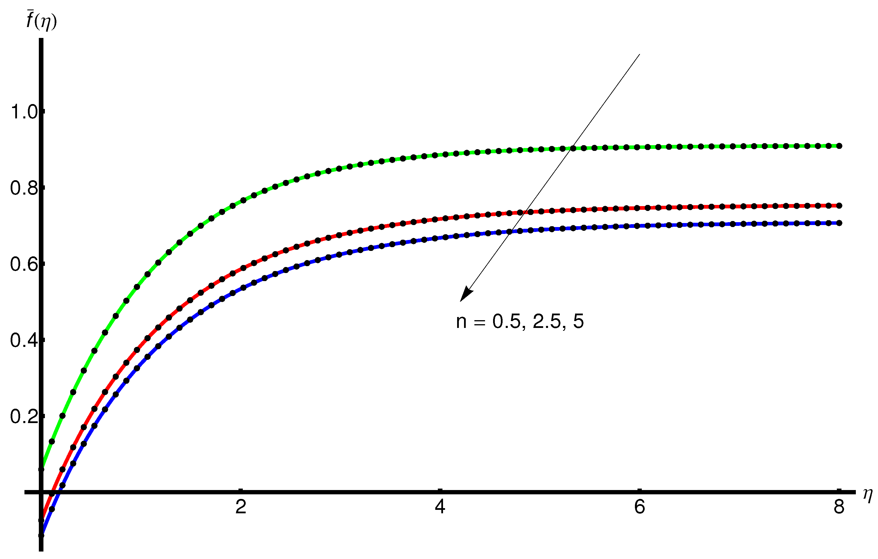
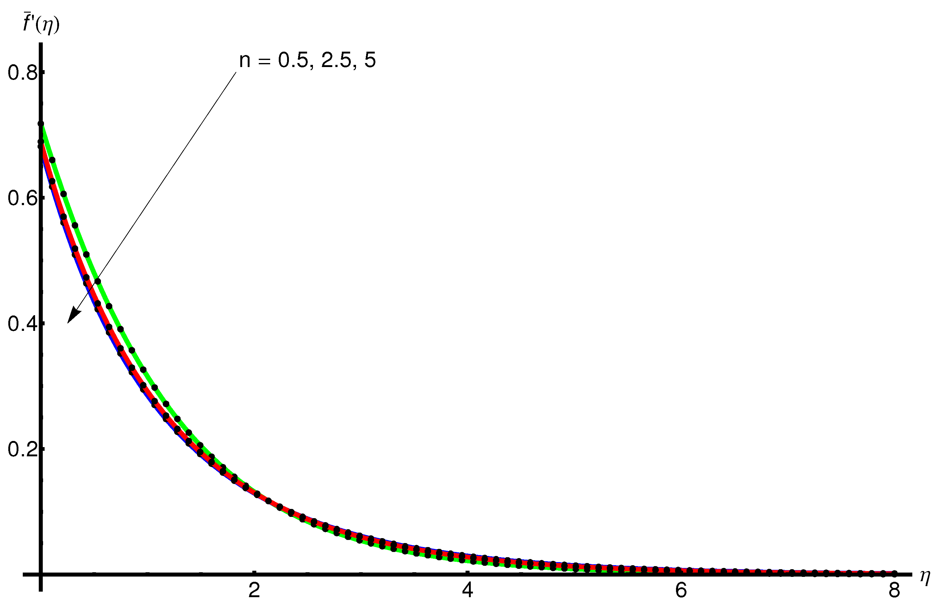
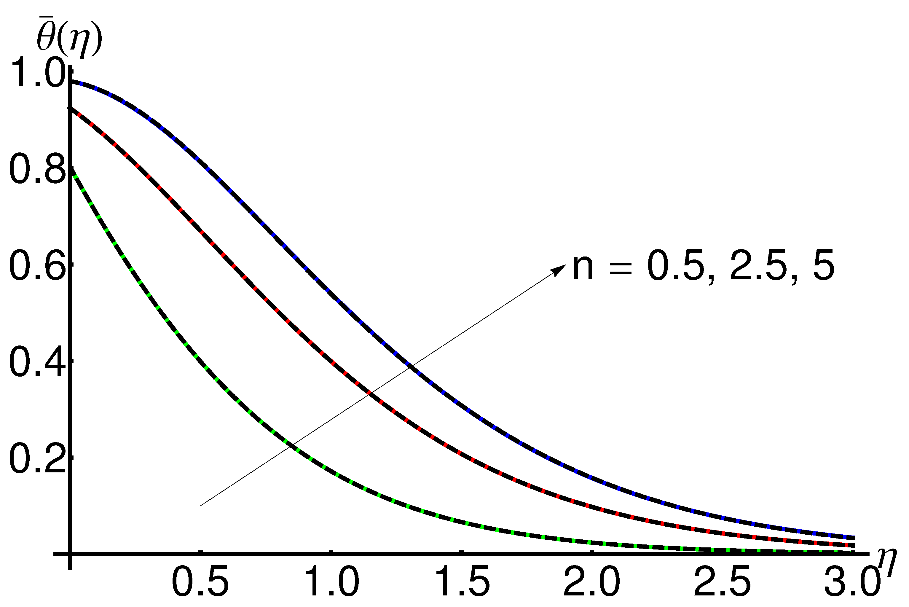
4.1. Influence of the Parameter n

The behaviour of the displacement and velocity f ¯ ( η ) and f ¯ ( η ) , respectively, with the increase in n for fixed values of R = 1 , P r = 6 , δ 2 = 0.2 , γ = 0.25 and δ 1 = 0.5 , are represented in Figure 2 and Figure 3, respectively. On the another hand from Figure 4 one can observe an increasing in temperature θ ¯ ( η ) with n.
Figure 2. The influence of n on the behaviour of the displacement f ¯ ( η ) (given by Equations (A3), (A17) and (A19) for γ = 0.25 , δ 1 = 0.5 : OHAM solution (thin lines) and numerical solution (dashing lines).
Mathematics 11 02199 g002
Figure 3. The influence of n on the behaviour of the velocity profile f ¯ ( η ) obtained from Equations (A3), (A17) and (A19) for γ = 0.25 , δ 1 = 0.5 : OHAM solution (thin lines) and numerical solution (dashing lines).
Mathematics 11 02199 g003
Figure 4. The influence of n on the behaviour of the temperature θ ¯ ( η ) given by Equations (A4), (A18) and (A20) for R = 1 , P r = 6 , δ 2 = 0.2 , γ = 0.25 , δ 1 = 0.5 : OHAM solution (thin lines) and numerical solution (dashing lines).
Mathematics 11 02199 g004
The slope and asymptotic limit decreases with the increasing values of η .

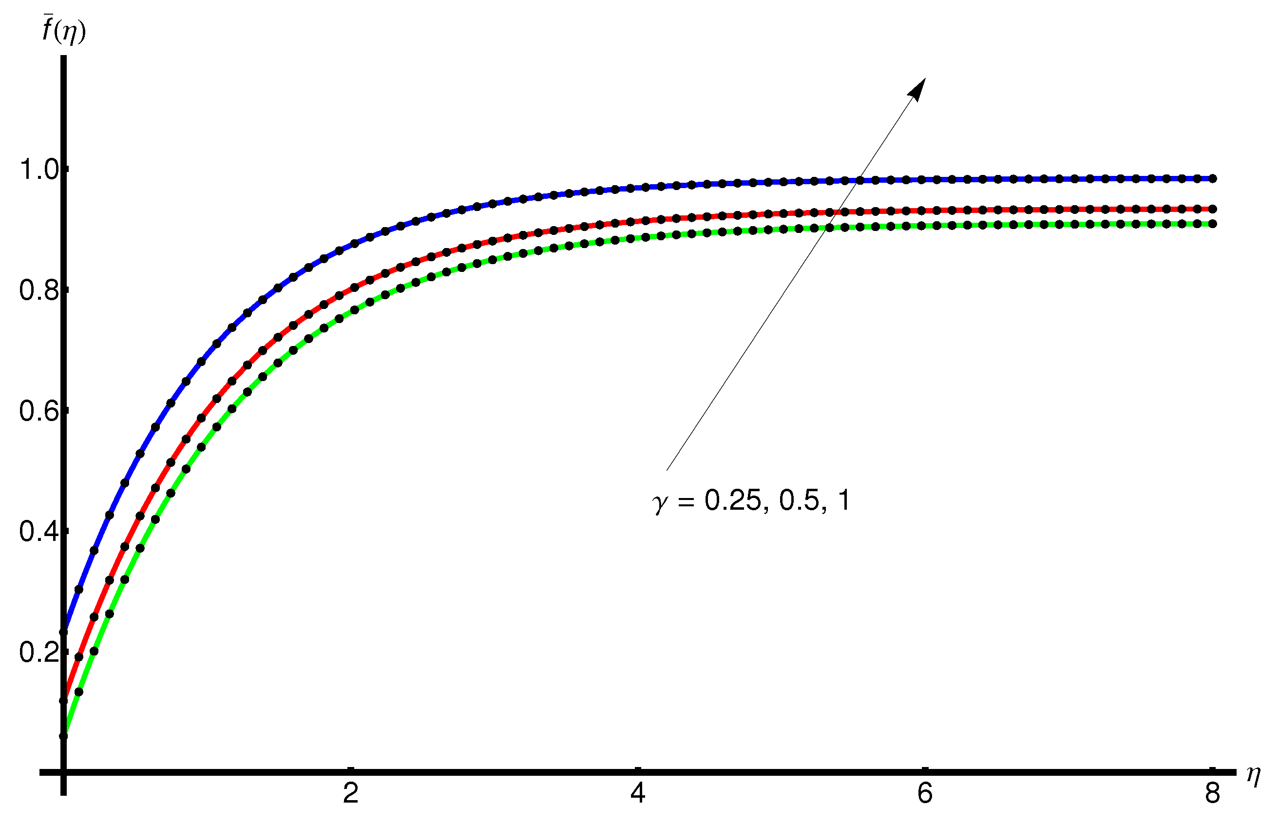
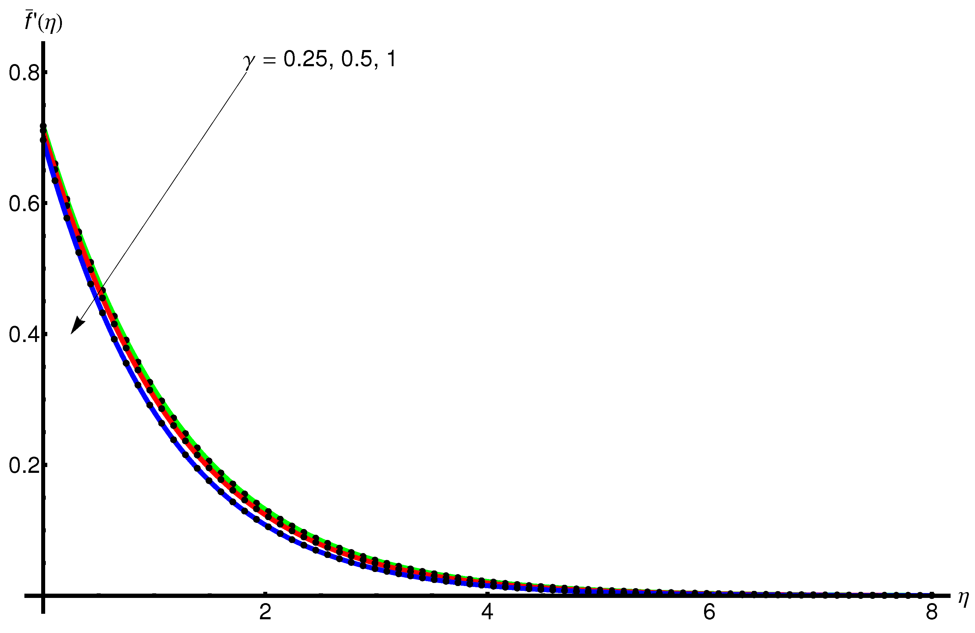
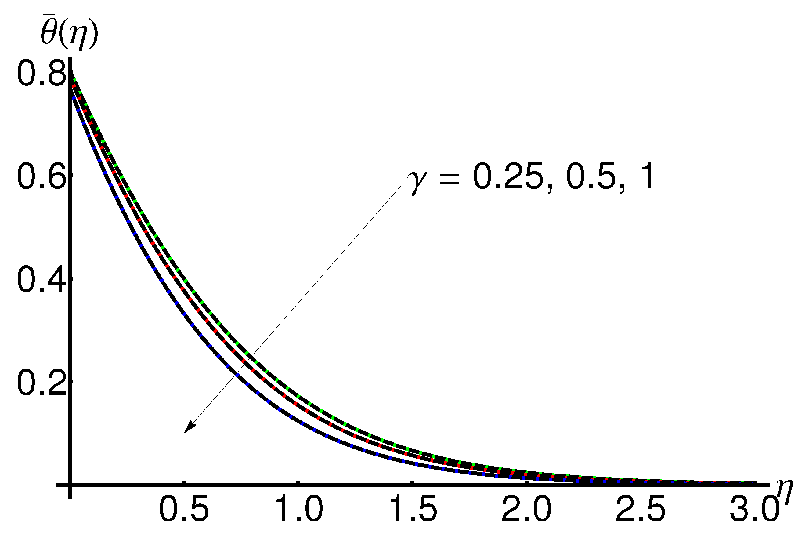
4.2. Influence of the Wall Thickness Parameter γ

Figure 5 and Figure 6 display the behaviour of the displacement f ¯ ( η ) and variation of the velocity f ¯ ( η ) , respectively, with increasing γ for fixed values of n = 0.5 , R = 1 , P r = 6 , and δ 2 = 0.2 , δ 1 = 0.5 ; while Figure 7 shows the variation in the temperature θ ¯ ( η ) decreases.
Figure 5. The influence of γ on the behaviour of the displacement f ¯ ( η ) given by Equations (A3), (A13) and (A15) for n = 0.5 , δ 1 = 0.5 : OHAM solution (thin lines) and numerical solution (dashing lines).
Mathematics 11 02199 g005
Figure 6. The influence of γ on the behaviour of the velocity profile f ¯ ( η ) obtained from Equations (A3), (A13) and (A15) for n = 0.5 , δ 1 = 0.5 : OHAM solution (thin lines) and numerical solution (dashing lines).
Mathematics 11 02199 g006
Figure 7. The influence of γ on the behaviour of the temperature θ ¯ ( η ) given by Equations (A4), (A14) and (A16) for n = 0.5 , R = 1 , P r = 6 , δ 2 = 0.2 , δ 1 = 0.5 : OHAM solution (thin lines) and numerical solution (dashing lines).
Mathematics 11 02199 g007
The slope and asymptotic limit increases for increasing values of η .

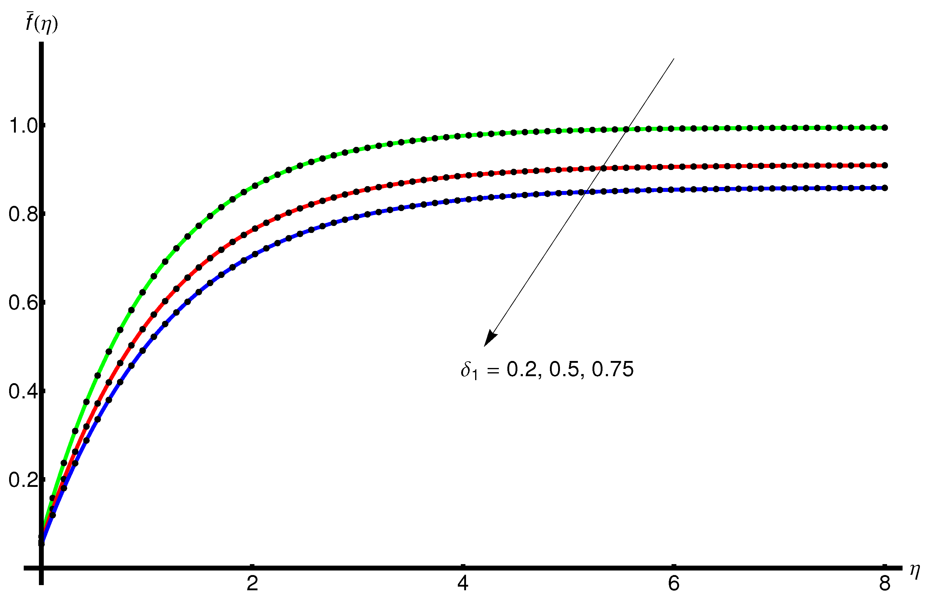
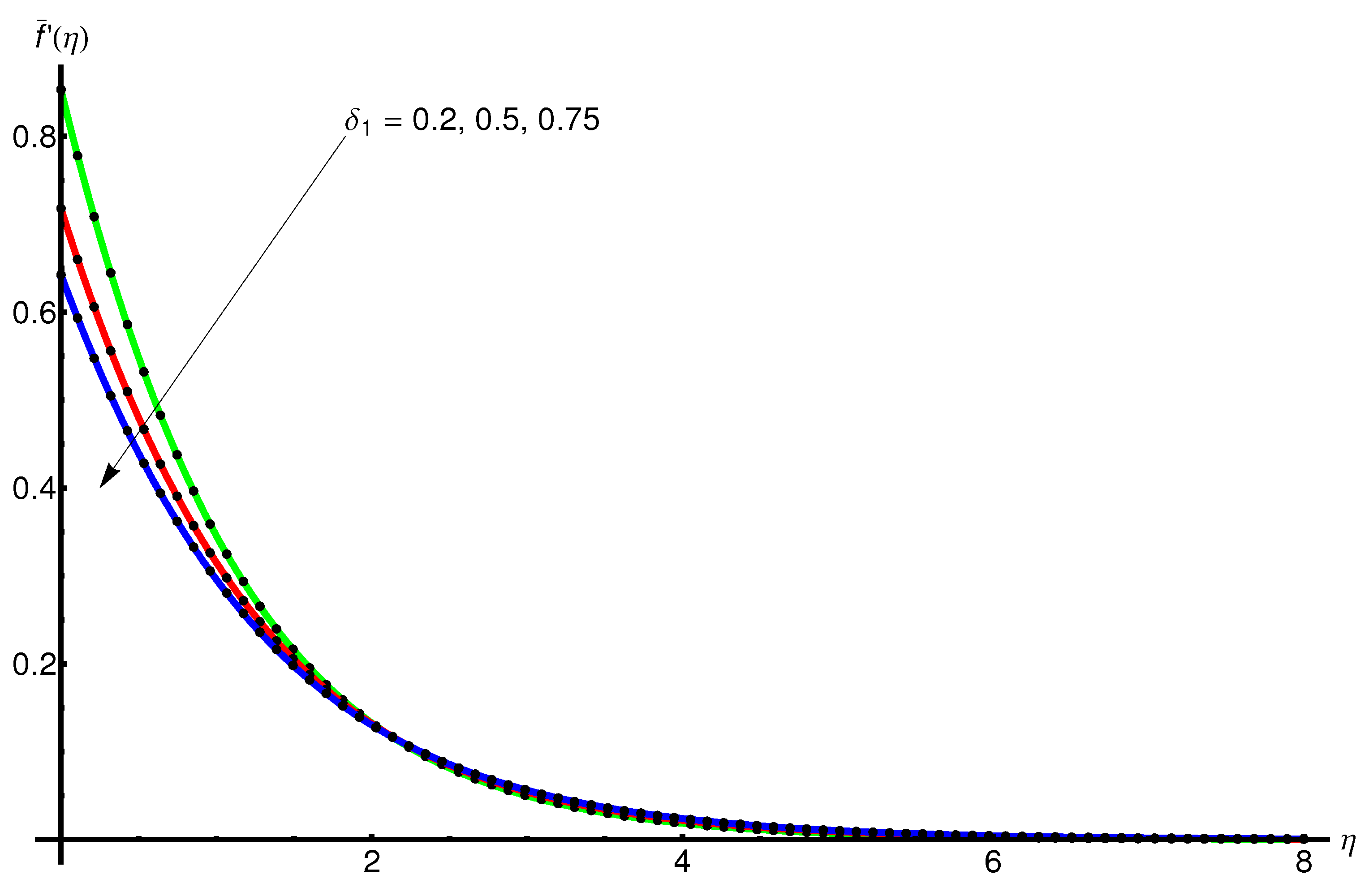
4.3. Influence of the Slip Parameter δ 1

The behaviour of the displacement and velocity f ¯ ( η ) and f ¯ ( η ) , respectively with the increasing of the parameter δ 1 for some fixed values of the parameters n = 0.5 , R = 1 , P r = 6 , δ 2 = 0.2 , γ = 0.25 , is represented in Figure 8 and Figure 9, respectively. In the Figure 10 can be observe an increasing of the temperature θ ¯ ( η ) with this parameter δ 1 .
Figure 8. The influence of the parameter δ 1 on the behaviour of the displacement f ¯ ( η ) given by Equations (A1), (A3) and (A11) for n = 0.5 , γ = 0.25 : OHAM solution (thin lines) and numerical solution (dashing lines).
Mathematics 11 02199 g008
Figure 9. The influence of δ 1 on the behaviour of the velocity profile f ¯ ( η ) obtained from Equations (A1), (A3) and (A11) for n = 0.5 , γ = 0.25 : OHAM solution (thin lines) and numerical solution (dashing lines).
Mathematics 11 02199 g009
Figure 10. Profile of the temperature θ ¯ ( η ) given by Equations (A2), (A4) and (A12) when increasing the slip parameter δ 1 for n = 0.5 , R = 1 , P r = 6 , δ 2 = 0.2 , γ = 0.25 : OHAM solution (thin lines) and numerical solution (dashing lines).
Mathematics 11 02199 g010
The slope and asymptotic limit decreases for increasing values of η .

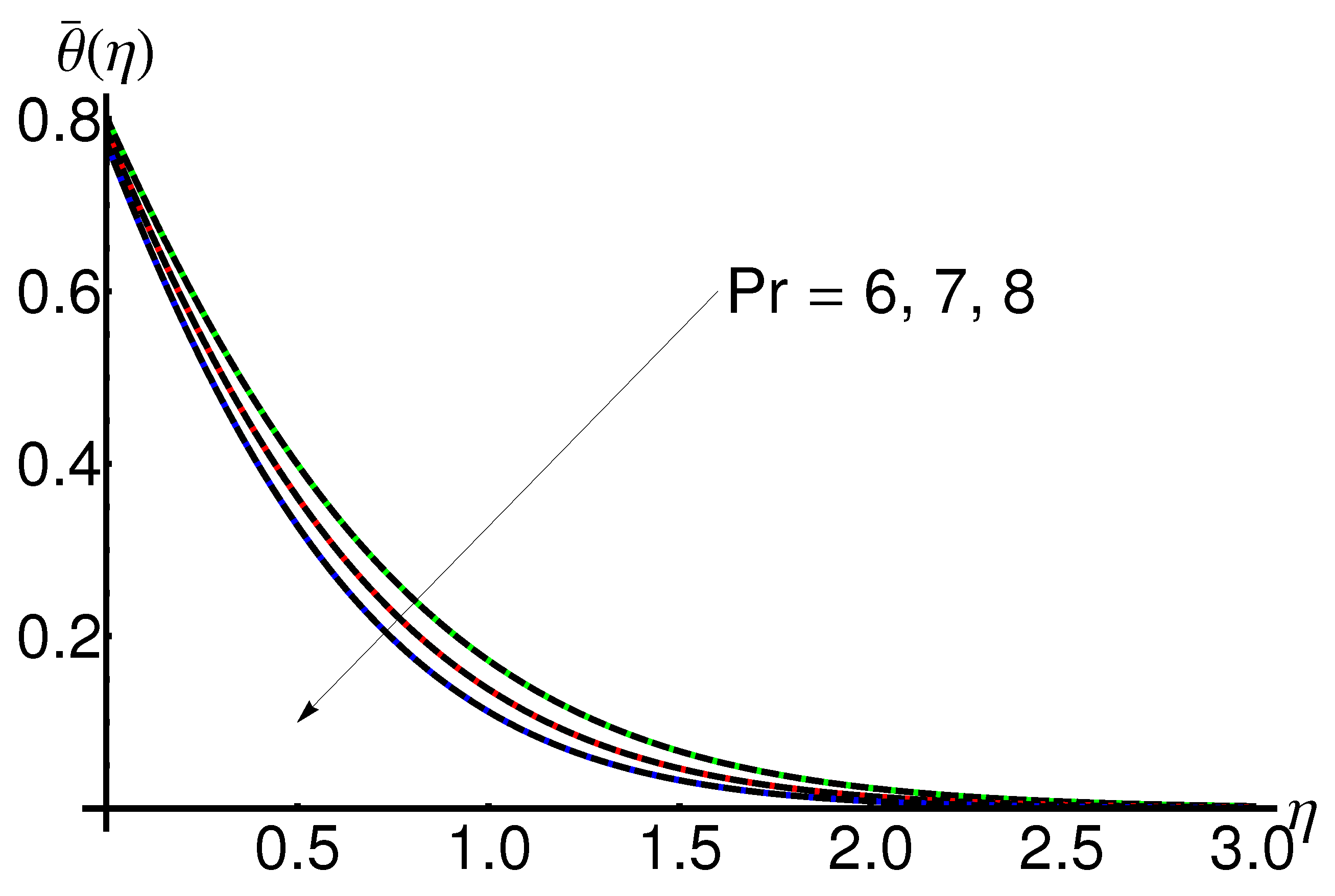
4.4. Influence of the Prandtl Number P r

Figure 11 displays the decrease in the temperature θ ¯ ( η ) with the increase in the Prandtl number P r for fixed values of n = 0.5 , R = 1 , δ 2 = 0.2 , γ = 0.25 , δ 1 = 0.5 .
Figure 11. Profile of the temperature θ ¯ ( η ) given by Equations (A4), (A5) and (A6) when increasing the Prandtl number P r for n = 0.5 , R = 1 , δ 2 = 0.2 , γ = 0.25 , δ 1 = 0.5 : OHAM solution (thin lines) and numerical solution (dashing lines).
Mathematics 11 02199 g011

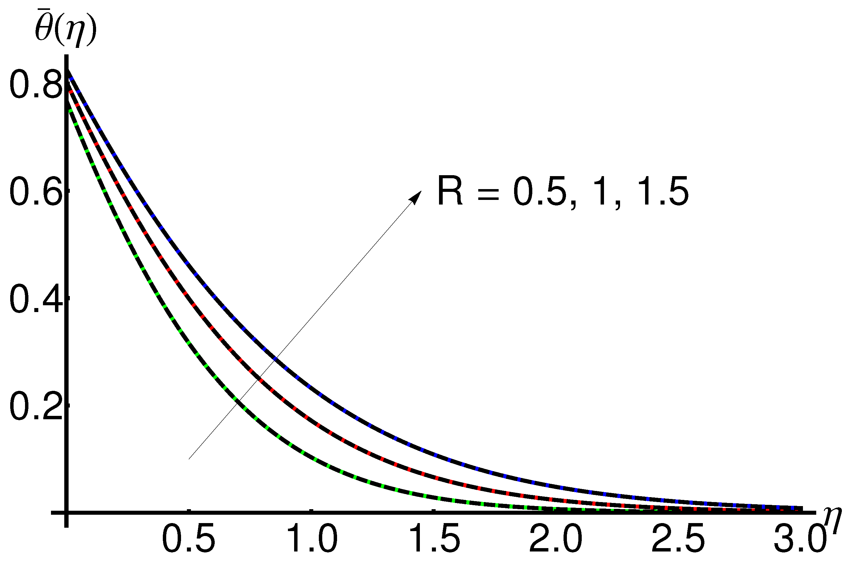
4.5. Influence of the Radiation Parameter R

Figure 12 shows the increase in temperature θ ¯ ( η ) when increasing the radiation number R for fixed values of n = 0.5 , P r = 6 , δ 2 = 0.2 , γ = 0.25 , δ 1 = 0.5 .
Figure 12. Profile of the temperature θ ¯ ( η ) given by Equations (A7), (A4) and (A8) when increasing the radiation parameter R for n = 0.5 , P r = 6 , δ 2 = 0.2 , γ = 0.25 , δ 1 = 0.5 : OHAM solution (thin lines) and numerical solution (dashing lines).
Mathematics 11 02199 g012

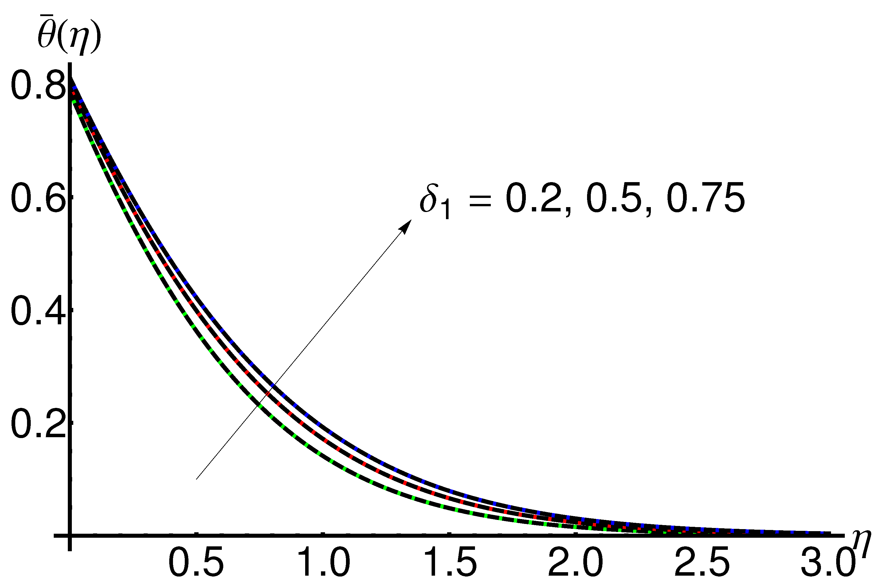
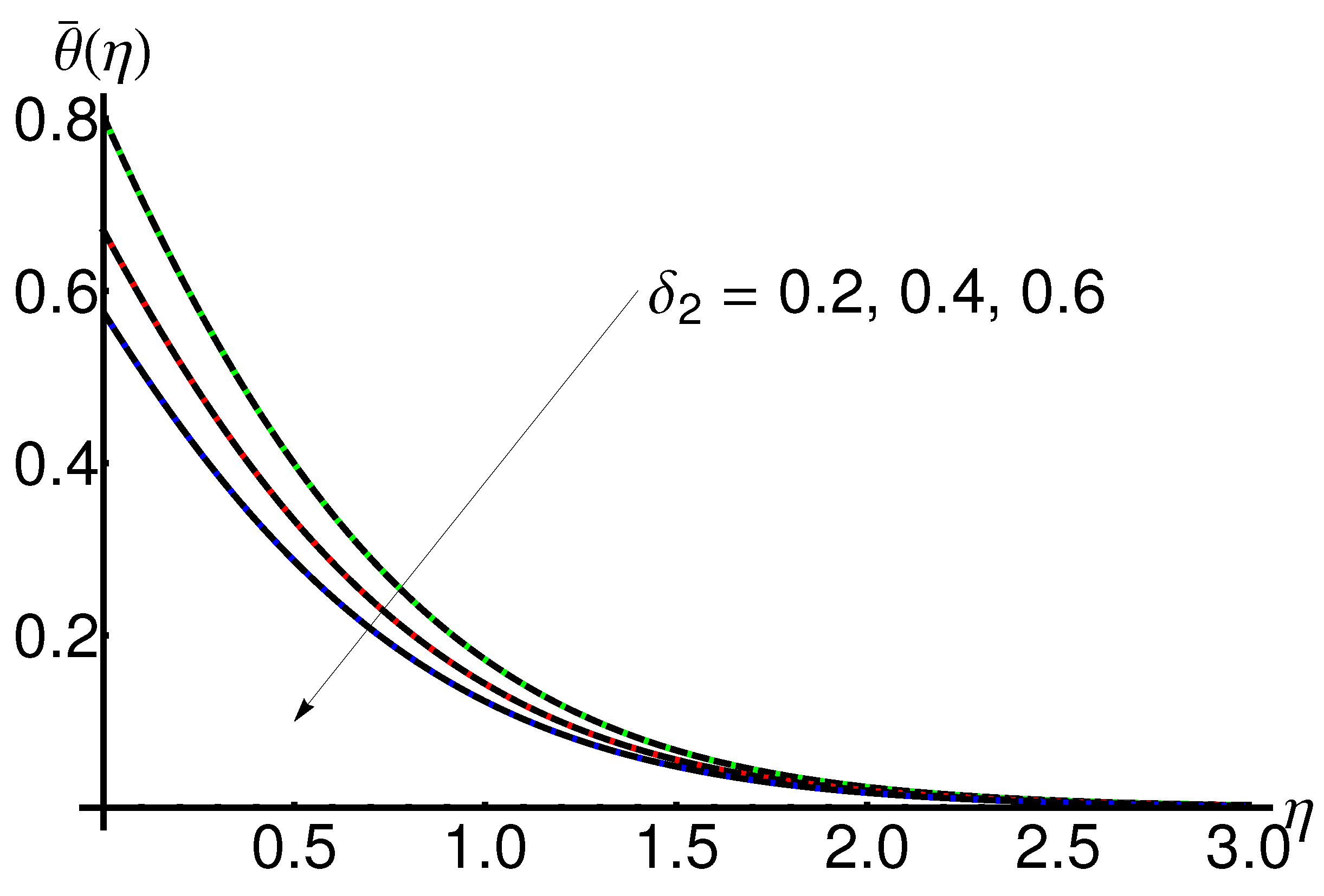
4.6. Influence of the Slip Thermal Parameter δ 2

From Figure 13 we notice that the variation in temperature.
Figure 13. Profile of the temperature θ ¯ ( η ) given by Equations (A4), (A9) and (A10) when increasing the slip thermal parameter δ 2 for n = 0.5 , R = 1 , P r = 6 , γ = 0.25 , δ 1 = 0.5 : OHAM solution (thin lines) and numerical solution (dashing lines).
Mathematics 11 02199 g013
The behaviour of the temperature θ ¯ ( η ) with increasing δ 2 for fixed values of n = 0.5 , R = 1 , P r = 6 , γ = 0.25 , δ 1 = 0.5 is depicted in Figure 13.
Table 5 presents in detail an error analysis by computing the integral of the square residual given by Equations (42) and (43).

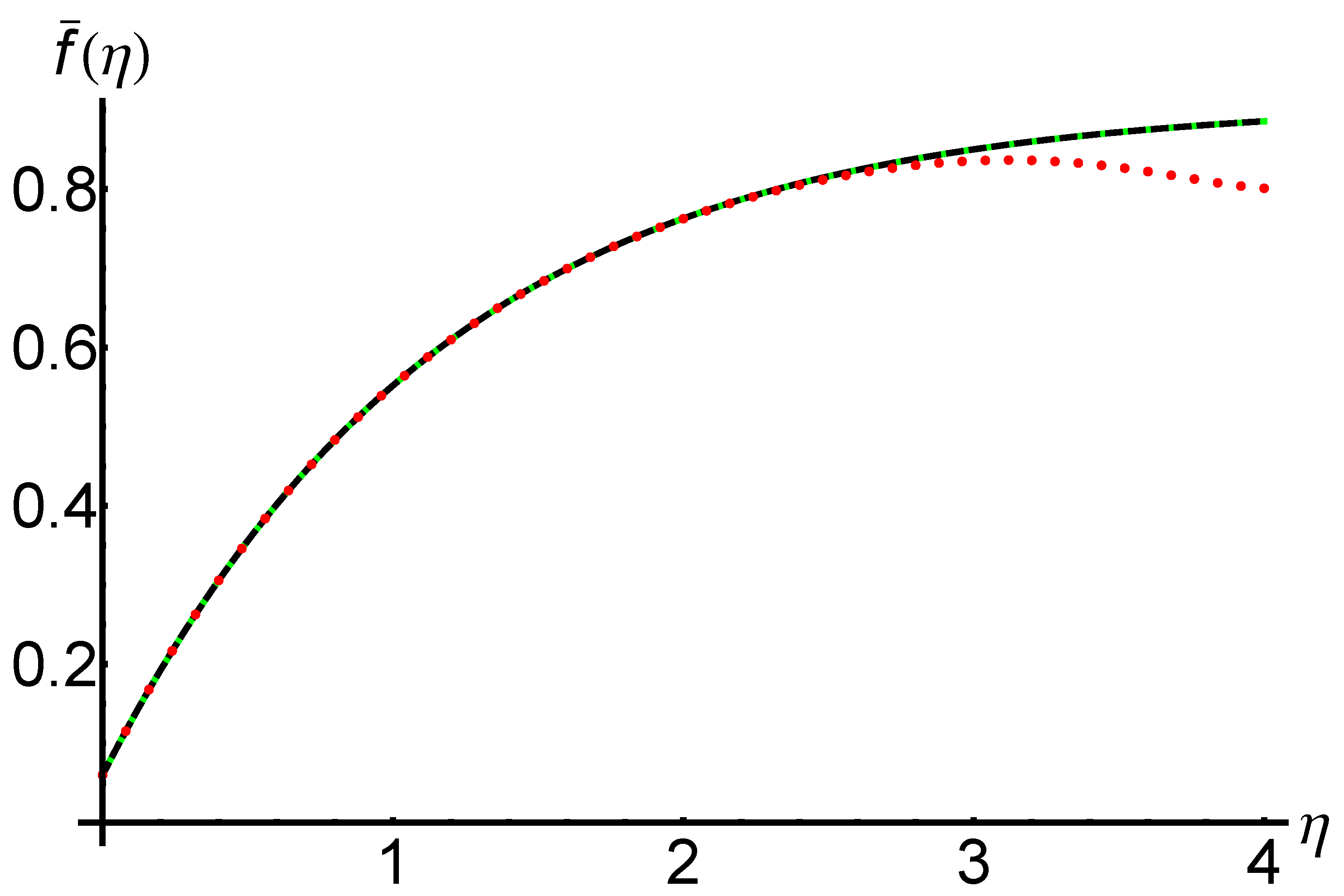
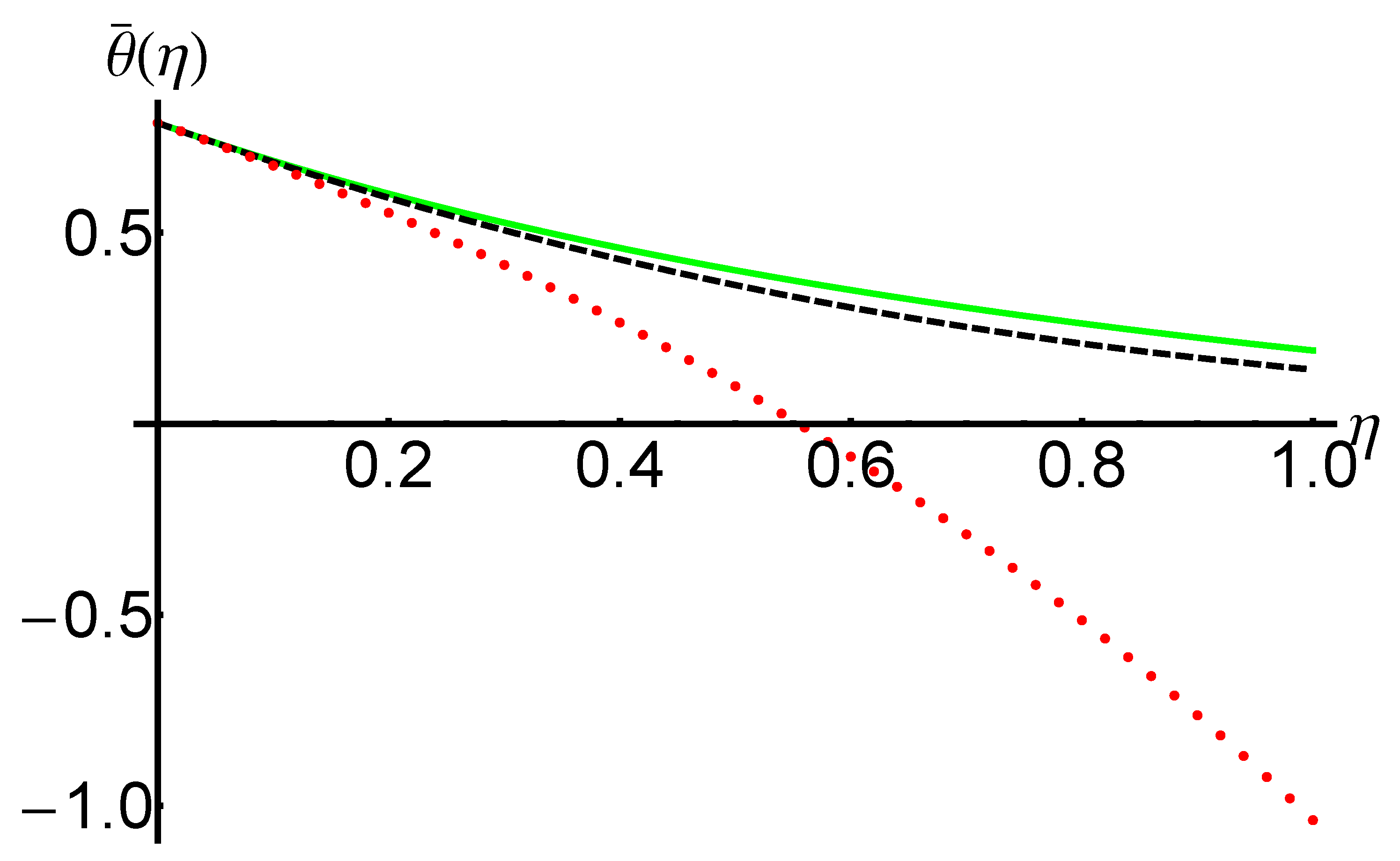
4.7. OHAM Solutions versus Iterative Solutions

A comparison between the OHAM solutions and corresponding iterative solutions obtained by the iterative method developed in [49] are presented highlighting the accuracy of the modified OHAM technique.
Equations (9) and (10) convert in the following system:
F 1 ( η ) = F 2 ( η ) F 2 ( η ) = F 3 ( η ) F 3 ( η ) = 2 n 1 + n F 2 2 ( η ) F 1 ( η ) F 3 ( η ) Θ 1 ( η ) = Θ 2 ( η ) Θ 2 ( η ) = P r 1 + 4 3 R · 1 n 1 + n · F 2 ( η ) Θ 1 ( η ) F 1 ( η ) Θ 2 ( η ) ,
where F 1 ( η ) = f ( η ) , F 2 ( η ) = f ( η ) , F 3 ( η ) = f ( η ) , Θ 1 ( η ) = θ ( η ) , Θ 2 ( η ) = θ ( η ) .
Integrating the system (44) over the interval [ 0 , η ] , results in:
F 1 ( η ) = F 1 ( 0 ) + 0 η F 2 ( s ) d s F 2 ( η ) = F 2 ( 0 ) + 0 η F 3 ( s ) d s F 3 ( η ) = F 3 ( 0 ) + 0 η 2 n 1 + n F 2 2 ( s ) F 1 ( s ) F 3 ( s ) d s Θ 1 ( η ) = Θ 1 ( 0 ) + 0 η Θ 2 ( s ) d s Θ 2 ( η ) = Θ 2 ( 0 ) + 0 η P r 1 + 4 3 R · 1 n 1 + n · F 2 ( s ) Θ 1 ( s ) F 1 ( s ) Θ 2 ( s ) d s .
The iterative procedure leads to:
F 1 , 0 ( η ) = F 1 ( 0 ) , F 1 , 1 ( η ) = N 1 ( F 1 , 0 , F 2 , 0 , F 3 , 0 , Θ 1 , 0 , Θ 2 , 0 ) = 0 η F 2 , 0 ( s ) d s , F 2 , 0 ( η ) = F 2 ( 0 ) , F 2 , 1 ( η ) = N 2 ( F 1 , 0 , F 2 , 0 , F 3 , 0 , Θ 1 , 0 , Θ 2 , 0 ) = 0 η F 3 , 0 ( s ) d s , F 3 , 0 ( η ) = F 3 ( 0 ) , F 3 , 1 ( η ) = N 3 ( F 1 , 0 , F 2 , 0 , F 3 , 0 , Θ 1 , 0 , Θ 2 , 0 ) = 0 η 2 n 1 + n F 2 , 0 2 ( s ) F 1 , 0 ( s ) F 3 , 0 ( s ) d s , Θ 1 , 0 ( η ) = Θ 1 ( 0 ) , Θ 1 , 1 ( η ) = N 4 ( F 1 , 0 , F 2 , 0 , F 3 , 0 , Θ 1 , 0 , Θ 2 , 0 ) = 0 η Θ 2 , 0 ( s ) d s , Θ 2 , 0 ( η ) = Θ 2 ( 0 ) , Θ 2 , 1 ( η ) = N 5 ( F 1 , 0 , F 2 , 0 , F 3 , 0 , Θ 1 , 0 , Θ 2 , 0 ) = 0 η P r 1 + 4 3 R · 1 n 1 + n · f 2 , 0 ( s ) θ 1 , 0 ( s ) f 1 , 0 ( s ) θ 2 , 0 ( s ) d s , F 1 , m ( η ) = N 1 i = 0 m 1 F 1 , i , i = 0 m 1 F 2 , i , i = 0 m 1 F 3 , i , i = 0 m 1 Θ 1 , i , i = 0 m 1 Θ 2 , i N 1 i = 0 m 2 F 1 , i , i = 0 m 2 F 2 , i , i = 0 m 2 F 3 , i , i = 0 m 2 Θ 1 , i , i = 0 m 2 Θ 2 , i , F 2 , m ( η ) = N 2 i = 0 m 1 F 1 , i , i = 0 m 1 F 2 , i , i = 0 m 1 F 3 , i , i = 0 m 1 Θ 1 , i , i = 0 m 1 Θ 2 , i N 2 i = 0 m 2 F 1 , i , i = 0 m 2 F 2 , i , i = 0 m 2 F 3 , i , i = 0 m 2 Θ 1 , i , i = 0 m 2 Θ 2 , i , F 3 , m ( η ) = N 3 i = 0 m 1 F 1 , i , i = 0 m 1 F 2 , i , i = 0 m 1 F 3 , i , i = 0 m 1 Θ 1 , i , i = 0 m 1 Θ 2 , i N 3 i = 0 m 2 F 1 , i , i = 0 m 2 F 2 , i , i = 0 m 2 F 3 , i , i = 0 m 2 Θ 1 , i , i = 0 m 2 Θ 2 , i , Θ 1 , m ( η ) = N 4 i = 0 m 1 F 1 , i , i = 0 m 1 F 2 , i , i = 0 m 1 F 3 , i , i = 0 m 1 Θ 1 , i , i = 0 m 1 Θ 2 , i N 4 i = 0 m 2 F 1 , i , i = 0 m 2 F 2 , i , i = 0 m 2 F 3 , i , i = 0 m 2 Θ 1 , i , i = 0 m 2 Θ 2 , i , Θ 2 , m ( η ) = N 5 i = 0 m 1 F 1 , i , i = 0 m 1 F 2 , i , i = 0 m 1 F 3 , i , i = 0 m 1 Θ 1 , i , i = 0 m 1 Θ 2 , i N 5 i = 0 m 2 F 1 , i , i = 0 m 2 F 2 , i , i = 0 m 2 F 3 , i , i = 0 m 2 Θ 1 , i , i = 0 m 2 Θ 2 , i , m 2 .
The solutions to Equations (9) and (10), using the iterative algorithm, can be written as:
F 1 i t e r ( η ) = m = 0 F 1 , m ( t ) , F 2 i t e r ( η ) = m = 0 F 2 , m ( η ) , F 3 i t e r ( η ) = m = 0 F 3 , m ( η ) ,
Θ 1 i t e r ( η ) = m = 0 Θ 1 , m ( η ) , Θ 2 i t e r ( η ) = m = 0 Θ 2 , m ( η ) .
The iterative solutions after six iterations and considering the initial conditions: F 1 ( 0 ) = γ 1 n 1 + n ( 1 + δ 1 · F 3 ( 0 ) ) , F 2 ( 0 ) = 1 + δ 1 · F 3 ( 0 ) , F 3 ( 0 ) = 0.5639692215 , Θ 1 ( 0 ) = 1 + δ 2 · Θ 2 ( 0 ) , Θ 2 ( 0 ) = 1.0625520610 (presented in Table 1 and Table 2) and the physical constants n = 0.5 , γ = 0.25 , δ 1 = 0.5 , R = 1 , P r = 6 , δ 2 = 0.2 , taking into account of the Algorithm (46), become:
f 1 i t e r ( η ) = m = 0 6 f 1 , m ( η ) = 0.0598346157 + 0.7180153892 η 0.2819846107 η 2 + + 0.0629070468 η 3 0.0065651516 η 4 0.0005435393 η 5 + 0.0002673026 η 6 , θ 1 i t e r ( η ) = m = 0 6 θ 1 , m ( η ) = 0.7874895877 1.0625520610 η 0.5312760305 η 2 0.1770920101 η 3 0.0442730025 η 4 0.0088546005 η 5 0.0014757667 η 6 .
Figure 14 and Figure 15 and Table 6, respectively, present a parallel between the OHAM solutions f ¯ O H A M and θ ¯ O H A M and the corresponding iterative solutions f 1 i t e r , θ 1 i t e r given in Equation (47). This comparative analysis highlights the efficiency and accuracy of the modified OHAM method using only one iteration.
The precision and efficiency of the OHAM method (using just one iteration) against the iterative method described in [49] (using six iterations) arising from the presented comparison.

5. Conclusions

Using the modified optimal homotopy asymptotic method (OHAM), the non-linear ODEs characterizing the radiative convective flow of a nanofluid over a stretching sheet in porous medium were analytically approximately solved. The equations were used to model physical phenomena related to fluid flow in the boundary layer, flow processes in porous media with applications in industry.
The dependence of the mass and heat transfer on the physical parameters was analytically and graphically investigated. The advantages of the OHAM procedure were highlighted by comparison with an iterative method. The impact of various parameters, such as: the velocity exponential factor n, the wall thickness parameter γ , the dimensionless velocity slip parameter δ 1 , the Prandtl number P r , the radiation parameter R, and the dimensionless temperature jump parameter δ 2 , is presented and summarized.
  • The effect of the increasing n enhances the stretching velocity and implies the elevation of the velocity boundary layer. Moreover, the temperature of the base fluid increases with n, leading the thickness of the thermal layer to increase;
  • If the wall thickness parameter γ increases, then the flow characteristics are considerably reduced and the temperature gradient is lowered;
  • An increase in the radiation parameter R causes an increase in the thickness of the thermal boundary layer supplying more heat to the base fluid;
  • An increase in the dimensionless temperature jump parameter δ 2 generates a high surface temperature, decreasing fluid conductance and increasing the thickness of the temperature profile;
  • The influence of Prandtl number P r on the temperature field in the presence/absence of joule heating is significant. The temperature and thermal boundary layer thickness were found to decrease;
  • An increase in the velocity slip parameter δ 1 implies a decrease in the boundary layer thickness, and a decrease in variation in the thermal boundary layer thickness.
The effects of the magnetic and electric fields for the radiative convective flow of a nanofluid over a stretching sheet in a porous medium will be analyzed in future work.

Author Contributions

Conceptualization, N.P.; data curation, R.-D.E. and N.P.; formal analysis, N.P.; investigation, R.-D.E. and R.B.; methodology, R.-D.E. and R.B.; software, R.-D.E.; supervision, N.P.; validation, R.-D.E. and N.P.; visualization, R.-D.E. and N.P.; writing—original draft, R.-D.E., R.B. and N.P. All authors have read and agreed to the published version of the manuscript.

Funding

This research received no external funding.

Institutional Review Board Statement

Not applicable.

Informed Consent Statement

Not applicable.

Data Availability Statement

Not applicable.

Conflicts of Interest

The authors declare no conflict of interest.

Nomenclature/Notation

SymbolsNames
u, v Velocity components
x, y Cartesian coordinates
nthe velocity power index parameter
K ( x ) Non-uniform permeability
k 0 Coefficient related to non-uniform permeability
u w ( x ) Velocity at the wall
T w ( x ) Wall temperature
T Environment temperature
u 0 , T 0 Reference velocity and reference temperature
ACoefficient related to stretching sheet
ν f Kinematical viscosity
TTemperature of the fluid
kThermal conductivity
α Thermal diffusivity of the nanofluid
( ρ c p ) f Specific heat capacitance
δ 1 Dimensional velocity slip parameter
δ 2 Dimensional temperature jump parameter
bthe Maxwell’s reflection coefficient
cthe thermal accommodation coefficient
λ the ratio of specific heats
ξ 1 , ξ 2 the mean free paths
q r Radiative heat flux
σ the Stefan-Boltzmann constant
k the mean absorption coefficient
P r Prandtl number
RRadiation parameter
γ the wall thickness parameter
δ 1 the dimensionless velocity slip parameter
δ 2 the dimensionless temperature jump parameter
R e x Reynolds number
η Independent dimensionless variable
f ( η ) Stream function
θ ( η ) Temperature
f ¯ ( η ) , θ ¯ ( η ) approximate analytical solution by means of the
modified Optimal Homotopy Asymptotic Method, called OHAM solutions

Appendix A

Example A1. n = 0.5 , γ = 0.25 , δ 1 = 0.2
f ¯ ( η ) = 0.9946172997 + ( 0.4139772770 η 2 0.6920469873 η 3 ) e 1.8862406706 η + + ( 0.3183621590 η 2 + 0.0365731067 η 3 ) e 1.1792663699 η + ( 0.1597270243 η 2 + 0.1524443533 η 3 ) × × e 1.4776951171 η + ( 0.0042329110 η 2 + 0.1548907491 η 3 ) e 1.9212671996 η + ( 0.0057258538 η 2 + + 0.6348504736 η 3 ) e 1.8637713840 η + ( 0.2568350851 η 2 + 0.0447155982 η 3 0.0040303481 η 4 ) × × e 1.2169940216 η + 0.1884050625 e 1.5173282040 η 1.1119121221 e 1.0245370781 η
Example A1.1. R = 1 , P r = 6 , δ 2 = 0.2
θ ¯ ( η ) = 1.3979533623 e 2.5662842234 η + ( 0.7874895997 1.6452099757 η ) e 1.3492902017 η + + ( 2.0002709304 0.2400457263 η 720.5014231601 η 2 ) e 2.4345962490 η + ( 2.4384372743 + + 0.4502081800 η 0.0255707584 η 2 ) e 1.2176022273 η + ( 1.8361197061 1.3495392047 η + + 719.6229654585 η 2 ) e 2.4352044546 η
Example A2. n = 0.5 , γ = 0.25 , δ 1 = 0.5
f ¯ ( η ) = 0.9097561021 + ( 0.2869318848 η 2 1.6372238807 η 3 ) e 2.1899790308 η + + ( 0.2080549264 η 2 0.7158289379 η 3 ) e 1.7080419443 η + ( 0.1211881336 η 2 + 0.1654718251 η 3 ) × × e 2.1387056347 η + ( 0.24616933011 η 2 + 0.6431173933 η 3 ) e 1.7009112737 η + ( 0.08245133002 η 2 + + 1.4569504253 η 3 ) e 2.1950662752 η + ( 0.5375166777 η 2 0.0782666024 η 3 + 0.0035238270 η 4 ) × × e 1.4790569937 η + 0.0767203339 e 1.6229736376 η 0.9266418203 e 0.9092299210 η
Example A2.1. R = 1 , P r = 6 , δ 2 = 0.2
θ ¯ ( η ) = 2.9456787532 e 2.7080923655 η + ( 0.8026925039 0.0843842327 η ) e 1.2290353718 η + + ( 0.2865440568 0.1115968792 η 0.9544376577 η 2 ) e 3.4387279254 η + ( 0.2484410860 0.3399227766 η 0.0944851935 η 2 ) e 1.7193639627 η + ( 2.4106936104 0.6098471315 η + + 1.3315794502 η 2 ) e 3.1984209564 η
Example A2.2. R = 1 , P r = 7 , δ 2 = 0.2
θ ¯ ( η ) = 1.0446433437 e 2.8306737159 η + ( 0.7872011518 0.0854789194 η ) e 1.3516167222 η + + ( 0.1496653624 + 0.0943652208 η 0.9855368948 η 2 ) e 3.7177556309 η + ( 1.2493619855 0.0005601138 η 0.1324666875 η 2 ) e 1.8588778154 η + ( 0.0550532792 + 1.3664899912 η + + 2.2018621320 η 2 ) e 3.3379348091 η
Example A2.3. R = 1 , P r = 8 , δ 2 = 0.2
θ ¯ ( η ) = 0.1677223956 e 2.9458417059 η + ( 0.7731817622 0.1092859450 η ) e 1.4667847122 η + + ( 1.4114699618 + 0.0170493137 η 0.2356907944 η 2 ) e 2.1459838851 η + ( 0.2793534893 + + 2.7301443316 η + 0.0963407657 η 2 ) e 4.2919677703 η + ( 0.9643940768 0.4778722401 η + + 3.2113280122 η 2 ) e 3.6250408788 η
Example A2.4. R = 0.5 , P r = 6 , δ 2 = 0.2
θ ¯ ( η ) = 32.5050621386 e 2.9901539452 η + ( 0.7679197587 + 87.0878602251 η ) e 1.5110969515 η + + ( 18.9741311586 + 1.7230004007 η 51.5082062592 η 2 ) e 2.9561265117 η + ( 6.1795235553 83.9041335593 η + 2.3062269196 η 2 ) e 1.4770695180 η + ( 19.7104545354 + 3.0879025287 η + + 53.8236497240 η 2 ) e 2.9541390361 η
Example A2.5. R = 1.5 , P r = 6 , δ 2 = 0.2
θ ¯ ( η ) = 2.7943652352 e 2.5295926714 η + ( 0.8263731124 0.0440600690 η ) e 1.0505356777 η + + ( 3.4497097475 0.2372528327 η 0.8627823196 η 2 ) e 2.8074987872 η + ( 0.4491261799 0.1800065186 η 0.0374528674 η 2 ) e 1.3284417935 η + ( 1.1044706922 + 0.1826813250 η + + 1.3808767029 η 2 ) e 2.6568835870 η
Example A2.6. R = 1 , P r = 6 , δ 2 = 0.4
θ ¯ ( η ) = 0.8867806614 e 2.7080926564 η + ( 0.6704146128 0.0618716928 η ) e 1.2290356627 η + + ( 0.1725218381 + 0.4069568146 η 1.2897712959 η 2 ) e 3.3156952475 η + ( 0.5248621360 0.1634234046 η 0.0671554042 η 2 ) e 1.6578476237 η + ( 0.5344403636 + 0.2452221795 η + + 2.0411668097 η 2 ) e 3.1369046174 η
Example A2.7. R = 1 , P r = 6 , δ 2 = 0.6
θ ¯ ( η ) = 4.3111040224 e 2.7080924834 η + ( 0.5755656406 0.0499255132 η ) e 1.2290354897 η + + ( 0.7275841885 + 0.4774478628 η 1.0862891617 η 2 ) e 3.3002236696 η + ( 0.7032195548 0.0340863577 η 0.0704533764 η 2 ) e 1.6501118348 η + ( 2.8803002790 1.2930950806 η + + 1.5769865882 η 2 ) e 3.1291688285 η
Example A3. n = 0.5 , γ = 0.25 , δ 1 = 0.75
f ¯ ( η ) = 0.8592108288 + ( 0.2070610330 η 2 + 0.0494307555 η 3 ) e 3.9537392065 η + + ( 0.5164824390 η 2 + 0.2578257758 η 3 ) e 2.3181363056 η + ( 0.5799578912 η 2 + 0.3827363388 η 3 ) × × e 3.1652763223 η + ( 0.6618028072 η 2 + 0.5796957297 η 3 ) e 2.4457198692 η + ( 0.3054908753 η 2 + + 0.8309626089 η 3 ) e 1.9160164060 η + ( 2.2707950460 η 2 + 0.2563475757 η 3 0.0073077125 η 4 ) × × e 1.6292493237 η + 0.0771076029 e 1.5141697991 η 0.8827650793 e 0.8602449854 η
Example A3.1. R = 1 , P r = 6 , δ 2 = 0.2
θ ¯ ( η ) = 5.079842172 e 2.7870969063 η + ( 0.8119720296 0.0833624724 η ) e 1.1578475826 η + + ( 1.8519889589 2.248636065 η 58.9934609300 η 2 ) e 3.2639449810 η + ( 0.4053898668 0.572633951 η 0.0637300121 η 2 ) e 1.6319724905 η + ( 3.6332430806 0.169372153 η + + 58.7914066303 η 2 ) e 3.2612218142 η
Example A4. n = 0.5 , γ = 0.5 , δ 1 = 0.5
f ¯ ( η ) = 0.9341156107 + ( 0.1390743471 η 2 3.0445723243 η 3 ) e 1.8605738407 η + + ( 0.0168469051 η 2 0.8833160929 η 3 ) e 1.5746217259 η + ( 0.2980880214 η 2 + 0.9671266866 η 3 ) × × e 1.8117128688 η + ( 0.3112024291 η 2 + 1.3296964905 η 3 ) e 1.5476443496 η + ( 1.4402441312 η 2 + + 2.4376920786 η 3 ) e 1.8668037907 η + ( 1.9273071396 η 2 + 0.2132086651 η 3 0.0073617636 η 4 ) × × e 1.2752945208 η + 0.1911543503 e 1.3857142064 η 1.0068062970 e 0.9690714949 η
Example A4.1. R = 1 , P r = 6 , δ 2 = 0.2
θ ¯ ( η ) = 0.7923635421 e 2.5945283111 η + ( 0.7912351664 0.0841178629 η ) e 1.3192337903 η + + ( 0.0816199379 0.0151786345 η 0.3254612303 η 2 ) e 3.6757124597 η + ( 1.0051353710 + + 0.0044161888 η 0.1554114241 η 2 ) e 1.8378562298 η + ( 0.1311518909 + 1.0117021785 η + + 1.0256949660 η 2 ) e 3.1131507507 η
Example A5. n = 0.5 , γ = 1 , δ 1 = 0.5
f ¯ ( η ) = 0.9843256617 + ( 0.4087537861 η 2 1.9758523669 η 3 ) e 2.5346694520 η ( 0.2678754951 η 2 0.0461245614 η 3 ) e 1.3840596643 η + ( 0.1608950512 η 2 + 0.1040290645 η 3 ) × × e 1.7198164890 η + ( 0.3297039955 η 2 + 0.7559361096 η 3 ) e 2.5769297131 η + ( 0.2142519563 η 2 + + 1.2935160470 η 3 ) e 2.4993619006 η + ( 0.0282217218 η 2 + 0.0034482635 η 3 0.0001162653 η 4 ) × × e 0.9878643345 η + 0.0946953564 e 1.5962582718 η 0.8468678287 e 1.0008855992 η
Example A5.1. R = 1 , P r = 6 , δ 2 = 0.2
θ ¯ ( η ) = 0.3597167846 e 2.4922451268 η + ( 0.7687126814 0.0954704839 η ) e 1.5043807923 η + + ( 0.0733310801 0.5892191368 η 0.3250643399 η 2 ) e 4.2045319974 η + ( 0.6308197167 0.5245411169 η 0.1430808772 η 2 ) e 2.1022659987 η + ( 0.1977718518 + 0.719415004 η 0.0137485551 η 2 ) e 3.0901303332 η
Example A6. n = 2.5 , γ = 0.25 , δ 1 = 0.5
f ¯ ( η ) = 0.7541685086 + ( 0.1158185725 η 2 0.4896838798 η 3 ) e 1.4427784905 η ( 0.2650992476 η 2 + 0.3422872956 η 3 ) e 1.4736158901 η ( 0.1361159150 η 2 + 0.0676280787 η 3 ) × × e 1.0977772584 η + ( 1.3141822854 η 2 + 0.1462983332 η 3 ) e 0.8922579152 η + ( 0.0555188904 η 2 + + 0.7846515973 η 3 ) e 1.4598016587 η + ( 1.6550977660 η 2 0.1805368975 η 3 + 0.0013656520 η 4 ) × × e 0.8898656083 η 0.2844288567 e 1.1651806024 η 0.5435807934 e 0.6581781498 η
Example A6.1. R = 1 , P r = 6 , δ 2 = 0.2
θ ¯ ( η ) = 257.5640986648 e 1.3008177481 η + ( 0.9240517880 0.0603655215 η ) e 0.4109521398 η + + ( 90.7596244009 23.8573078674 η 178261.5920432491 η 2 ) e 1.7797390335 η + + ( 83.86711073782 + 17.9038061212 η 1.3679947656 η 2 ) e 0.8898734252 η + + ( 82.9373635260 42.7181083865 η + 178250.3752803285 η 2 ) e 1.7797468505 η
Example A7. n = 5 , γ = 0.25 , δ 1 = 0.5
f ¯ ( η ) = 0.7091673617 + ( 1.0214662661 η 2 2.2024525481 η 3 ) e 2.2888220109 η + + ( 2.4363488175 η 2 1.1479916570 η 3 ) e 1.7177888735 η + ( 0.6130211922 η 2 + 0.6413035628 η 3 ) × × e 1.8425247246 η + ( 1.4513883678 η 2 + 0.7195007290 η 3 ) e 1.7920503662 η + ( 0.7683703580 η 2 + + 2.6073338327 η 3 ) e 2.2759261623 η + ( 6.2905950018 η 2 + 0.6005060191 η 3 + 0.0344934779 η 4 ) × × e 1.7145828237 η 0.1121579464 e 1.5730824623 η 0.7106162433 e 0.7109424735 η
Example A7.1. R = 1 , P r = 6 , δ 2 = 0.2
θ ¯ ( η ) = 200.8827425077 e 1.8163880731 η + ( 0.9800452497 0.0204310992 η ) e 0.1018052494 η + + ( 2.0670795815 0.0778464180 η 0.0657019518 η 2 ) e 0.4314687029 η + ( 0.5106635013 0.0843065638 η 0.0100304601 η 2 ) e 0.2157343514 η + ( 202.4391585879 + 25.2916387690 η + + 2.7198689180 η 2 ) e 1.9303171751 η

References

  1. Vishalakshi, A.B.; Maranna, T.; Shettar Mahabaleshwar, U.; Laroze, D. An Effect of MHD on Non–Newtonian Fluid Flow over a Porous Stretching/Shrinking Sheet with Heat Transfer. Appl. Sci. 2022, 12, 4937. [Google Scholar] [CrossRef]
  2. Maranna, T.; Sneha, K.N.; Mahabaleshwar, U.S.; Sarris, I.E.; Karakasidis, T.E. An Effect of Radiation and MHD Newtonian Fluid over a Stretching/Shrinking Sheet with CNTs and Mass Transpiration. Appl. Sci. 2022, 12, 5466. [Google Scholar] [CrossRef]
  3. Sarma, S.; Ahmed, N. Thermal Diffusion Effect on Unsteady MHD Free Convective Flow Past a Semi- Infinite Exponentially Accelerated Vertical Plate in a Porous Medium. Can. J. Phys. 2022, 100, 437–451. [Google Scholar] [CrossRef]
  4. Mahabaleshwar, U.S.; Anusha, T.; Laroze, D.; Said, N.M.; Sharifpur, M. An MHD Flow of Non–Newtonian Fluid Due to a Porous Stretching/Shrinking Sheet with Mass Transfer. Sustainability 2022, 14, 7020. [Google Scholar] [CrossRef]
  5. Akhtar, S.; Almutairi, S.; Nadeem, S. Impact of heat and mass transfer on the Peristaltic flow of non-Newtonian Casson fluid inside an elliptic conduit: Exact solutions through novel technique. Chin. J. Phys. 2022, 78, 194–206. [Google Scholar] [CrossRef]
  6. Safdar, M.; Ijaz Khan, M.; Khan, R.A.; Taj, S.; Abbas, F.; Elattar, S.; Galal, A.M. Analytic solutions for the MHD flow and heat transfer in a thin liquid film over an unsteady stretching surface with Lie symmetry and homotopy analysis method. Waves Random Complex Media 2022, 33, 442–460. [Google Scholar] [CrossRef]
  7. Krishna, M.V. Analytical study of chemical reaction, Soret, Hall and ion slip effects on MHD flow past an infinite rotating vertical porous plate. Waves Random Complex Media 2022. [Google Scholar] [CrossRef]
  8. Reddy, Y.D.; Mebarek-Oudina, F.; Goud, B.S.; Ismail, A.I. Radiation, Velocity and Thermal Slips Effect Toward MHD Boundary Layer Flow Through Heat and Mass Transport of Williamson Nanofluid with Porous Medium. Arab. J. Sci. Eng. 2022, 47, 16355–16369. [Google Scholar] [CrossRef]
  9. Abbas, A.; Jeelani, M.B.; Alharthi, N.H. Darcy-Forchheimer Relation Influence on MHD Dissipative Third-Grade Fluid Flow and Heat Transfer in Porous Medium with Joule Heating Effects: A Numerical Approach. Processes 2022, 10, 906. [Google Scholar] [CrossRef]
  10. Elbashbeshy, E.M.A.; Asker, H.G. Fluid flow over a vertical stretching surface within a porous medium filled by a nanofluid containing gyrotactic microorganisms. Eur. Phys. J. Plus 2022, 137, 541. [Google Scholar] [CrossRef]
  11. Nuwairan, M.A.; Hafeez, A.; Khalid, A.; Syed, A. Heat generation/absorption effects on radiative stagnation point flow of Maxwell nanofluid by a rotating disk influenced by activation energy. Case Stud. Therm. Eng. 2022, 35, 102047. [Google Scholar] [CrossRef]
  12. Abbas, N.; UrRehman, K.; Shatanawi, W.; Malik, M.Y. Numerical study of heat transfer in hybrid nanofluid flow over permeable nonlinear stretching curved surface with thermal slip. Int. Commun. Heat Mass Transf. 2022, 135, 106107. [Google Scholar] [CrossRef]
  13. Hossein, S.; Ahmadi, N.; Jabbary, A. Effects of applying brand-new designs on the performance of PEM fuel cell and water flooding phenomena. Iran. J. Chem. Chem. Eng. 2022, 41, 618–634. [Google Scholar]
  14. Aziz, T.; Aziz, A.; Shams, M.; Bahaidarah, H.M.S.; Alie, H. Entropy analysis with the Cattaneo-Christov heat flux model for the Powell-Eyring nanofluid flow over a stretching surface. Waves Random Complex Media 2022. [Google Scholar] [CrossRef]
  15. Jena, S.; Mishra, S.R.; Aghaeiboorkheili, M.; Pattnaik, P.K.; Muduli, K. Impact of Newtonian heating on the conducting Casson fluid flow past a stretching cylinder. J. Interdiscip. Math. 2022, 25, 2401–2416. [Google Scholar] [CrossRef]
  16. Sultana, U.; Mushtaq, M.; Muhammad, T. Numerical simulation for stagnation-point flow of nanofluid over a spiraling disk through porous media. Waves Random Complex Media 2022. [Google Scholar] [CrossRef]
  17. Gul, T.; Saeed, A. Nonlinear mixed convection couple stress tri-hybrid nanofluids flow in a Darcy-Forchheimer porous medium over a nonlinear stretching surface. Waves Random Complex Media 2022. [Google Scholar] [CrossRef]
  18. Khan, M.R.; Algarni, S.; Alqahtani, T.; Alsallami, S.A.M.; Saeed, T.; Galal, A.M. Numerical analysis of a time-dependent aligned MHD boundary layer flow of a hybrid nanofluid over a porous radiated stretching/shrinking surface. Waves Random Complex Media 2022. [Google Scholar] [CrossRef]
  19. Rasool, G.; Shah, N.A.; El-Zahar, E.R.; Wakif, A. Numerical investigation of EMHD nanofluid flows over a convectively heated riga pattern positioned horizontally in a Darcy-Forchheimer porous medium: Application of passive control strategy and generalized transfer laws. Waves Random Complex Media 2022. [Google Scholar] [CrossRef]
  20. Reddy, P.B.A.; Jakeer, S.; Basha, H.T.; Reddy, S.R.; Kumar, T.M. Multi-layer artificial neural network modeling of entropy generation on MHD stagnation point flow of Cross-nanofluid. Waves Random Complex Media 2022. [Google Scholar] [CrossRef]
  21. Fadaei, M.; Izadi, M.; Assareh, E.; Ershadi, A. Melting process of PCM with Carreau—Yasuda non-Newtonian behavior in a shell and tube heat exchanger occupied by anisotropic porous medium. Int. J. Numer. Heat Fluid Flow 2022. ahead-of-print. [Google Scholar] [CrossRef]
  22. Wang, J.; Mustafa, Z.; Siddique, I.; Ajmal, M.; Jaradat, M.M.M.; Rehman, S.U.; Ali, B.; Muhammad Ali, H. Computational Analysis for Bioconvection of Microorganisms in Prandtl Nanofluid Darcy-Forchheimer Flow across an Inclined Sheet. Nanomaterials 2022, 12, 1791. [Google Scholar] [CrossRef] [PubMed]
  23. Abdal, S.; Siddique, I.; Din, I.S.U.; Ahmadian, A.; Hussain, S.; Salimi, M. Significance of magnetohydrodynamic Williamson Sutterby nanofluid due to a rotating cone with bioconvection and anisotropic slip. J. Appl. Math. Mech. 2022, 102, e202100503. [Google Scholar] [CrossRef]
  24. Wahid, N.S.; Arifin, N.; Khashi’Ie, N.S.; Pop, I.; Bachok, N.; Hafidzuddin, M.E.H. Hybrid nanofluid stagnation point flow past a slip shrinking Riga plate. Chin. J. Phys. 2022, 78, 180–193. [Google Scholar] [CrossRef]
  25. Meenakumari, R.; Lakshminarayana, P. MHD 3D flow of powell eyring fluid over a bidirectional non-linear stretching surface with temperature dependent conductivity and heat absorption/generation. Proc. Inst. Mech. Eng. Part E J. Process Mech. Eng. 2022, 236, 2580–2588. [Google Scholar] [CrossRef]
  26. Alharbi, K.A.M.; Khan, M.R.; Ould Sidi, M.; Algelany, A.M.; Elattar, S.; Ahammad, N.A. Investigation of hydromagnetic bioconvection flow of Oldroyd-B nanofluid past a porous stretching surface. Biomass Convers. Biorefin. 2022, 13, 4331–4342. [Google Scholar] [CrossRef]
  27. Krishna, M.; Vajravelu, K. Rotating MHD flow of second grade fluid through porous medium between two vertical plates with chemical reaction, radiation absorption, Hall, and ion slip impacts. Biomass Convers. Biorefin. 2022. [Google Scholar] [CrossRef]
  28. Tayebi, T. Analysis of the local non-equilibria on the heat transfer and entropy generation during thermal natural convection in a non-Darcy porous medium. Int. Commun. Heat Mass Transf. 2022, 135, 106133. [Google Scholar] [CrossRef]
  29. Zainal, N.A.; Nazar, R.; Naganthran, K.; Pop, I. Stability Analysis of Unsteady Hybrid Nanofluid Flow over the Falkner-Skan Wedge. Nanomaterials 2022, 12, 1771. [Google Scholar] [CrossRef]
  30. Jha, B.; Samaila, G. Similarity solution for boundary layer flow near a moving vertical porous plate with combined effects of nonlinear thermal radiation and suction/injection having convective surface boundary condition. Proc. Inst. Mech. Eng. J. Mech. Eng. Sci. 2022, 236, 8926–8934. [Google Scholar] [CrossRef]
  31. Meena, O.P.; Janapatla, P. Mixed convection flow over a vertical cone saturated porous medium with double dispersion effect. Appl. Math. Comput. 2022, 430, 127072. [Google Scholar] [CrossRef]
  32. Naseem, T.; Fatima, U.; Munir, M.; Shahzad, A.; Kausar, N.; Nisar, K.S.; Saleel, C.A.; Abbas, M. Joule heating and viscous dissipation effects in hydromagnetized boundary layer flow with variable temperature. Case Stud. Therm. Eng. 2022, 35, 102083. [Google Scholar] [CrossRef]
  33. Veeram, G.; Poojitha, P.; Katta, H.; Hemalatha, S.; Babu, M.J.; Raju, C.S.; Shah, N.A.; Yook, S.J. Simulation of Dissipative Hybrid Nanofluid (PEG-Water + ZrO2 + MgO) Flow by a Curved Shrinking Sheet with Thermal Radiation and Higher Order Chemical Reaction. Mathematics 2022, 10, 1706. [Google Scholar] [CrossRef]
  34. Kumar, G.V.; Rehman, K.U.; Kumar, R.V.M.S.S.K.; Shatanawi, W. Unsteady magnetohydrodynamic nanofluid flow over a permeable exponentially surface manifested with non-uniform heat source/sink effects. Waves Random Complex Media 2022. [Google Scholar] [CrossRef]
  35. Rooman, M.; Jan, M.A.; Shah, Z.; Vrinceanu, N.; Bou, S.F.; Iqbal, S.; Deebani, W. Entropy Optimization on Axisymmetric Darcy-Forchheimer Powell-Eyring Nanofluid over a Horizontally Stretching Cylinder with Viscous Dissipation Effect. Coatings 2022, 12, 749. [Google Scholar] [CrossRef]
  36. Goud, B.S.; Reddy, Y.D.; Mishra, S. Joule heating and thermal radiation impact on MHD boundary layer Nanofluid flow along an exponentially stretching surface with thermal stratified medium. Proc. Inst. Mech. Eng. J. Nanomater. Nanoeng. Nanosyst. 2022, 23977914221100961. [Google Scholar] [CrossRef]
  37. Manvi, B.; Tawade, J.; Biradar, M.; Noeiaghdam, S.; Fernandez-Gamiz, U.; Govindan, V. The effects of MHD radiating and non-uniform heat source/sink with heating on the momentum and heat transfer of Eyring-Powell fluid over a stretching. Results Eng. 2022, 14, 100435. [Google Scholar] [CrossRef]
  38. Ali, A.; Khan, H.S.; Saleem, S.; Hussan, M. EMHD Nanofluid Flow with Radiation and Variable Heat Flux Effects along a Slandering Stretching Sheet. Nanomaterials 2022, 12, 3872. [Google Scholar] [CrossRef]
  39. Marinca, V.; Herisanu, N. The Optimal Homotopy Asymptotic Method—Engineering Applications; Springer: Berlin/Heidelberg, Germany, 2015. [Google Scholar]
  40. Marinca, V.; Ene, R.D.; Marinca, B.; Negrea, R. Different approximations to the solution of upper-convected Maxwell fluid over a porous stretching plate. Abstr. Appl. Anal. 2014, 2014, 139314. [Google Scholar] [CrossRef]
  41. Ene, R.D.; Marinca, V. Approximate solutions for steady boundary layer MHD viscous flow and radiative heat transfer over an exponentially porous stretching sheet. Appl. Math. Comput. 2015, 269, 389–401. [Google Scholar] [CrossRef]
  42. Ene, R.D.; Szabo, M.A.; Danoiu, S. Viscous flow and heat transfer over a permeable shrinking sheet with partial slip. Mater. Plast. 2015, 52, 408–412. [Google Scholar]
  43. Marinca, V.; Ene, R.D. Dual approximate solutions of the unsteady viscous flow over a shrinking cylinder with Optimal Homotopy Asymptotic Method. Adv. Math. Phys. 2014, 2014, 417643. [Google Scholar] [CrossRef]
  44. Ene, R.D.; Pop, N. Dual approximate solutions for the chemically reactive solute transfer in a viscous fluid flow. Waves Random Complex Media 2022, 1–23. [Google Scholar] [CrossRef]
  45. Ene, R.D.; Petrisor, C. Some mathematical approaches on the viscous flow problem on a continuous stretching surface: Nonlinear stability and dual approximate analytic solutions. AIP Conf. Proc. 2020, 2293, 350004. [Google Scholar]
  46. Devi, S.P.A.; Thiyagarajan, M. Steady nonlinear hydromagnetic flow and heat transfer over a stretching surface of variable temperature. Heat Mass Transf. 2006, 42, 671–677. [Google Scholar] [CrossRef]
  47. Sulochana, C.; Sandeep, N. Dual Solutions for Radiative MHD Forced Convective Flow of a Nanofluid over a Slendering Stretching Sheet in Porous Medium. J. Nav. Archit. Mar. Eng. 2015, 12, 115–124. [Google Scholar] [CrossRef]
  48. Brewster, M.Q. Thermal Radiative Transfer Properties; John Wiley and Sons: Hoboken, NJ, USA, 1972. [Google Scholar]
  49. Daftardar-Gejji, V.; Jafari, H. An iterative method for solving nonlinear functional equations. J. Math. Anal. Appl. 2006, 316, 753–763. [Google Scholar] [CrossRef]
Figure 1. Schematic diagram of the physical model.
Mathematics 11 02199 g001
Figure 14. Profile of the approximate analytical solution f ¯ ( η ) , of Equation (9) given by Equation (A3), the iterative solution f 1 i t e r ( η ) given by Equation (47) and the corresponding numerical solution: numerical solution (thin lines), OHAM solution (dashing lines), and iterative solution (dotted curve).
Mathematics 11 02199 g014
Figure 15. Profile of the approximate analytical solution θ ¯ ( η ) , of Equation (10) given by Equation (A4), the corresponding numerical solution and the iterative solution θ 1 i t e r ( η ) given by Equation (47). numerical solution (thin lines), OHAM solution (dashing lines), and iterative solution (dotted curve).
Mathematics 11 02199 g015
Table 1. Values of the skin-friction coefficient f ¯ ( 0 ) obtained from Equation (31) by the OHAM and numerical results, for different values of n, γ and δ 1 (relative errors: ϵ f ( 0 ) = | f n u m e r i c a l ( 0 ) f ¯ O H A M ( 0 ) | ).
n γ δ 1 f n u m e r i c a l ( 0 ) f ¯ O H A M ( 0 ) ϵ f ( 0 )
0.50.250.2−0.7333855928−0.733385591810 9
0.50.250.5−0.5639692215−0.563969220510 9
0.50.250.75−0.4764796954−0.476479694410 9
0.50.50.5−0.5784360410−0.578436031010 8
0.510.5−0.6070808644−0.607080863410 9
2.50.250.5−0.6216320348−0.621632024810 8
50.250.5−0.6367180731−0.636718063110 8
Table 2. Values of the heat transfer coefficient θ ¯ ( 0 ) obtained from Equation (41) by the OHAM and numerical results, for different values of n, γ , δ 1 , R, P r , and δ 2 (relative errors: ϵ θ ( 0 ) = | θ n u m e r i c a l ( 0 ) θ ¯ O H A M ( 0 ) | ).
n γ δ 1 R P r δ 2 θ n u m e r i c a l ( 0 ) θ ¯ O H A M ( 0 ) ϵ θ ( 0 )
0.50.250.5160.2−0.9865380801−0.986537980110 7
0.50.250.5170.2−1.0639948406−1.063994740610 7
0.50.250.5180.2−1.1340917886−1.134091688610 7
0.50.250.50.560.2−1.1604012664−1.160401256410 8
0.50.250.5160.2−0.9865380801−0.986537980110 7
0.50.250.51.560.2−0.8681344977−0.868134487710 8
0.50.250.5160.2−0.9865380801−0.986537980110 7
0.50.250.5160.4−0.8239638179−0.823963717910 7
0.50.250.5160.6−0.7073908656−0.707390765610 7
2.50.250.5160.2−0.3797410596−0.38859669968.855639 · 10 3
50.250.5160.2−0.0997737511−0.099773741110 8
0.50.50.5160.2−1.0438247676−1.043824667610 7
0.510.5160.2−1.1564371927−1.156437092710 7
0.50.250.2160.2−1.0625520610−1.062552051010 8
0.50.250.75160.2−0.9401404517−0.940140351710 7
Table 3. Values of the analytic approximate solutions f ¯ ( η ) and f ¯ ( η ) from Equation (A3) and θ ¯ ( η ) from Equation (A4) obtained by the OHAM and corresponding numerical results, for the values n = 0.5 , γ = 0.25 , δ 1 = 0.5 , R = 1 , P r = 6 , and δ 2 = 0.2 (relative errors: ϵ f = | f n u m e r i c a l f ¯ O H A M | , ϵ f = | f n u m e r i c a l f ¯ O H A M | , ϵ θ = | θ n u m e r i c a l θ ¯ O H A M | ).
η f n u m e r i c a l f n u m e r i c a l θ n u m e r i c a l
00.05983461570.71801538920.8026923839
0.250.22267123550.58839877170.5777496315
0.50.35578630620.47980726170.3992585355
0.750.46410798100.38961543060.2660675341
10.55191328780.31526051480.1718011819
1.250.62285760400.25434569690.1079932864
1.50.68002475960.20470290480.0663727087
1.750.72598843920.16442146530.0400386110
20.76287749260.13185236780.0237854503
2.250.79244001190.10559549140.0139544082
2.50.81610291110.08447735890.0081040406
2.750.83502533510.06752469210.0046679539
30.85014524780.05393679090.0026710288
η f ¯ O H A M f ¯ O H A M θ ¯ O H A M
00.05983461580.71801538970.8026925039
0.250.22267123790.58839877260.5777441370
0.50.35578630720.47980723190.3992654139
0.750.46410797680.38961541960.2660663722
10.55191328710.31526054360.1717963676
1.250.62285760840.25434574480.1079934516
1.50.68002476410.20470288700.0663767004
1.750.72598843790.16442144140.0400411532
20.76287748820.13185236840.0237837569
2.250.79244000800.10559549990.0139493825
2.50.81610291110.08447738120.0080983796
2.750.83502533960.06752470360.0046641177
30.85014525470.05393679450.0026702523
η ε f ε f ε θ
04.166664 · 10 11 5.000001 · 10 10 1.200000 · 10 7
0.252.338812 · 10 9 8.500138 · 10 10 5.494534 · 10 6
0.59.967847 · 10 10 2.982538 · 10 8 6.878355 · 10 6
0.754.282139 · 10 9 1.095087 · 10 8 1.161948 · 10 6
16.948758 · 10 10 2.880794 · 10 8 4.814365 · 10 6
1.254.403408 · 10 9 4.789489 · 10 8 1.652118 · 10 7
1.54.521325 · 10 9 1.783327 · 10 8 3.991710 · 10 6
1.751.352115 · 10 9 2.390061 · 10 8 2.542265 · 10 6
24.420232 · 10 9 6.084595 · 10 10 1.693424 · 10 6
2.253.888561 · 10 9 8.512293 · 10 9 5.025664 · 10 6
2.52.571165 · 10 12 2.233086 · 10 8 5.660951 · 10 6
2.754.493213 · 10 9 1.154742 · 10 8 3.836207 · 10 6
36.906006 · 10 9 3.618723 · 10 9 7.764704 · 10 7
Table 4. Comparison between the limit-value f ( ) : = lim η f ( η ) obtained from Equation (31) by the OHAM and numerical results, for different values of n, γ and δ 1 (relative errors: ϵ f ( ) = | f n u m e r i c a l ( ) f ¯ O H A M ( ) | ).
n γ δ 1 f n u m e r i c a l ( ) f ¯ O H A M ( ) ϵ f ( )
0.50.250.20.99461720100.9946172997 10 7
0.50.250.50.90975599210.9097561021 10 7
0.50.250.750.85921072870.8592108288 10 7
0.50.50.50.9341155120.93411561078 10 7
0.510.50.9843255610.98432566179 10 7
2.50.250.50.7541684090.75416850866 10 7
50.250.50.7091667120.709167361756.496262 · 10 7
Table 5. Integral of the square residual given by Equations (42) and (43) obtained by the OHAM for different values of n, γ and δ 1 , R, P r and δ 2 .
n γ δ 1 0 R f ¯ 2 ( η ) d η R P r δ 2 0 R θ ¯ 2 ( η ) d η
0.50.250.25.485739 · 10 11 160.21.079470 · 10 5
0.50.250.55.503738 · 10 13 160.24.737834 · 10 7
170.29.489441 · 10 7
180.21.914615 · 10 6
0.560.23.598609 · 10 5
1.560.23.601433 · 10 9
160.42.265013 · 10 7
160.61.504156 · 10 7
0.50.250.752.848927 · 10 10 160.21.139814 · 10 6
0.50.50.51.486587 · 10 11 160.21.787740 · 10 7
0.510.57.256022 · 10 11 160.22.676813 · 10 7
2.50.250.52.500198 · 10 11 160.21.100465 · 10 3
50.250.53.167293 · 10 9 160.28.243077 · 10 5
Table 6. Comparison between the approximate analytical solution f ¯ ( η ) given by Equation (A3), the iterative solution f 1 i t e r ( η ) given by Equation (47) and the corresponding numerical solution.
η f n u m e r i c a l f ¯ O H A M f 1 iter
00.05983461570.05983461580.0598346157
2/50.30577672120.30577672840.3057767378
4/50.48318468660.48318469390.4831857409
6/50.60986183680.60986184460.6098707988
8/50.69962618280.69962617500.6996239146
20.76287751610.76287748820.7625577448
12/50.80726613260.80726609550.8051757704
14/50.83832697300.83832693100.8300974997
16/50.86001708210.86001702600.8362170948
18/50.87514158730.87514150520.8221825663
40.88567718830.88567707600.8010064019
Disclaimer/Publisher’s Note: The statements, opinions and data contained in all publications are solely those of the individual author(s) and contributor(s) and not of MDPI and/or the editor(s). MDPI and/or the editor(s) disclaim responsibility for any injury to people or property resulting from any ideas, methods, instructions or products referred to in the content.

