Article

Analysis of the Vibro-Impact Nonlinear Damped and Forced Oscillator in the Dynamics of the Electromagnetic Actuation

1
Department of Mechanics and Strength of Materials, University Politehnica Timisoara, 300006 Timisoara, Romania
2
Center for Advanced and Fundamental Technical Research, Department of Electromechanics and Vibration, Romanian Academy, 300223 Timisoara, Romania
3
Department of Applied Electronics, University Politehnica Timisoara, 300006 Timisoara, Romania
4
Faculty of Technical Sciences, University of Novi Sad, 21000 Novi Sad, Serbia
*
Author to whom correspondence should be addressed.
Mathematics 2023, 11(9), 2194; https://doi.org/10.3390/math11092194
Submission received: 5 April 2023 / Revised: 22 April 2023 / Accepted: 27 April 2023 / Published: 6 May 2023
(This article belongs to the Special Issue Nonlinear Vibration Theory and Mechanical Dynamics)

Abstract

:
In this work, the effect of vibro-impact nonlinear, forced, and damped oscillator on the dynamics of the electromagnetic actuation (EA) near primary resonance is studied. The vibro-impact regime is given by the presence of the Hertzian contact. The EA is supplied by a constant current generating a static force and by an actuation generating a fast alternative force. The deformations between the solids in contact are supposed to be elastic and the contact is maintained. In this study, a single degree of freedom nonlinear damped oscillator under a static normal load is considered. An analytical approximate solution of this problem is obtained using the Optimal Auxiliary Functions Method (OAFM). By means of some auxiliary functions and introducing so-called convergence-control parameters, a very accurate approximate solution of the governing equation can be obtained. We need only the first iteration for this technique, applying a rigorous mathematical procedure in finding the optimal values of the convergence-control parameters. Local stability by means of the Routh-Hurwitz criteria and global stability using the Lyapunov function are also studied. It should be emphasized that the amplitude of AC excitation voltage is not considered much lower than bias voltage (in contrast to other studies). Also, the Hertzian contact coupled with EA is analytically studied for the first time in the present work. The approximate analytical solution is determined with a high accuracy on two domains. Local stability is established in five cases with some cases depending on the trace of the Jacobian matrix and of the discriminant of the characteristic equation. In the study of global stability, the estimate parameters which are components of the Lyapunov function are given in a closed form and a graphical form and therefore the Lyapunov function is well-determined.

1. Introduction

In the last decades, analysis of the Hertzian contact and electromagnetic actuation (EA) has been caried out in several studies since these are present in various engineering systems such as railway wheel contact [1], the automotive sector [2], gear drive [3], energy dissipation in mechanical systems, and in mechanisms transforming movements of rotations or translations [4]. EA are used in some engineering applications such as hydraulic valves, small heart pumps, electric door, power relays, etc.
Some studies are devoted to the problem of resonances (principal, subharmonic, or superharmonic). Mann et al. [5] investigated the dynamic behavior of a pendulum with finite time impact events that is modeled by Hertz’s contact law. Periodic, subharmonic, quasi-periodic, and chaotic behavior are experimentally and numerically explored. Ma et al. [6] explored Hertzian contact problem of a dynamic response for a spherical plane contact interface with contact loss. The clearance-type nonlinearity is given by the contact loss with harmonic balance approximation. Liaudet and Sabot [7] considered the principal, subharmonic, and superharmonic resonances for the case of a loaded sphere-plane Hertzian contact. Also, the classical contact problem of normal contact between a rigid sphere and elastic half-space is examined by Popov [8]. An exact solution of this problem in the framework of the half-space approximation is obtained and the deformations in an elastic half-space are given by the stress activity upon its surface.
The Hertzian distribution was assumed by Axinte [9] for the normal surface contact load over a circular contact area. The rail-wheel contact problems have been analyzed by means of the three-dimensional finite element models. The bodies of the contact problem are the standard rail UIC60 and the standard wheel UICORE. Liaudet and Rigaud [10] proposed a numerical procedure based on shooting method and multiple scale method and then experimental technique in the study of superharmonic resonance for an impacting Hertzian oscillator. The practical way for controlling the vibroimpact dynamics of a Hertzian contact forced oscillator is the introduction of a fast harmonic base displacement, as showed by Bichri et al. [11], which is generally around some microns. Different aspects of vibroimpact dynamics in a forced Hertzian contact oscillator such as the effect of time delay, control of a forced impact Hertzian contact near resonances [12], contact stiffness modulation in contact-mode atomic force microscopy [13], and the effect of EA on contact loss in a Hertzian contact oscillator [14] are intensively investigated.
Belhaq et al. [15] considered the effect of EAs on the dynamics of a periodically excited cantilever beam, numerically by means of finite element method, analytically based on a perturbation analysis and experimentally using a test rig. The force induced by the EA lead to a softening behavior into the system. The role of a high frequency AC of an EA and the dynamics of an excited cantilever beam is explored by Bichri et al. [16] by means of analytical and numerical procedures near the primary resonance. Pereira et al. [17] applied EA to a rotating machine on the learning position, and a proportional derivative controller is used for deriving the desired control laws. The Timoshenko beam theory and finite elements method are considered.
To enhance the actuation performance controlled by a harmonic input signal, Zhang et al. [18] proposed a novel bistable nonlinear EA with elastic boundary. The bifurcation features have been derived in terms of the inclined spring stiffness, the input signal frequency and amplitude. The effect of nonlinear actuator dynamics and an aeroelastic simulation model of a flexible wing with control surface are examined by Tang et al. [19]. Zhang and Li [20] proposed a compound scheme based on an improved active disturbance controller and nonlinear compensation for an electromechanical actuator system. The Lu Gre model and hysteresis inverse model are used to compensate for the friction and backlash phenomenon. Simulation and experiment are presented to validate the effectiveness of the proposed method.
The multiple scale method with the force-deflection characteristic approximated by a third order Taylor series expansion is proposed by Xiao et al. [21]. Then, harmonic balance method is employed to determine the natural frequency for free vibrations of an elastic body by interaction of a mass with a Hertzian contact stiffness. The Hertzian contact given by a dry contact between a rigid flat surface and elastic cylinder is considered by Ali [22]. The two-dimensional numerical simulation on the subsurface stress field in Hertzian contact under pure sliding condition for different speeds and coefficients of friction is studied applying normal load and angular speed for the cylinder. Quazi et al. [23] proposed a strip-based local approach to extend the FASTSIM algorithm to non-elliptical contact cases. Different settings for the traction bound are explored to determine their influence on the contact stresses, creep forces, and the limits of the saturation zone in the case of wheel-rail contact. The absolute error in the normalized creep forces is used as the quantity of interest and found to be consistent with other known results. Ciulli et al. [24] compared the results obtained by theoretical and finite element analysis of the point contact of non-conformal and conformal pairs made of spheres, caps, and spherical seats. The displacement and force relation were investigated by varying the geometrical parameters, the materials, the boundary conditions and the friction coefficient.
Constandinou et al. [25] established that in the case of multi-spherical approach, there exist two sources for error directly affecting the normal contact forces. These are due to the difference between the true particle shape and the multi-spherical approximation and other arises from the contact model used in the Discrete Element Modelling simulations. Wu et al. [26] analyzed the validity of the Hertz theory for large deformations by means of nanoindentation tests and finite element method. They proved that the loading load-displacement relation still holds for δ/R as large as 0.66 with a maximum principal strain of 46.6%. Vouaillat et al. [27] studied the rolling contact fatigue in spur gears taking into account the spur gear material geometry, the contact pressure fields and several parameters such as friction, sliding coefficient, load variation and roughness. A fatigue criterion based on rolling contact fatigue micro-cracks nucleation at grain boundaries is proposed. Yousuf [28] examined the effect of contact load on the bending deflection considering a system with spring stiffness and viscous damping to reduce the bending deflection on the cam profile. The dynamic response has been obtained by means of Solid Works software based on the contact parameters. Finite element analysis was used to calculate the bending deflection of the cam profile numerically. A new impact-driving piezoelectric vibration energy harvesting for low-frequency and broadband vibration harvesting is proposed by Cao et al. [29]. The results of the numerical simulation and vibration test demonstrate the advantages of the vibration energy harvesting for the lower resonance frequency and the higher output power. Zhang et al. [30] proposed an enhanced vibro-impact energy harvester using acoustic back holes for scavenging low-frequency vibration energy.
The present work is motivated by the need to add new results to this narrow field of research. The first objective of this work is to find an approximate analytical solution for the nonlinear differential equation of the vibro-impact oscillator under the influence of the two symmetric EA force near the primary resonance. The vibro-impact regime is given by the presence of the Hertzian contact supposing that the contact is elastic and is maintained. The Optimal Auxiliary Functions Method (OAFM) is applied to determine an analytic approximate solution of the problem. The main novelties of the proposed approach are the presence of some auxiliary functions, the introduction of the convergence-control parameters, the original construction of the initial and first iteration, and the freedom to choose the procedure for determining the optimal values of the convergence-control parameters. The proposed technique is proved to be very accurate, simple, effective, and easy to be applied using only the first iteration.
The second objective of the paper is to perform an analysis of the stability of the nonlinear model by means of the eigenvalues of the Jacobian matrix. The signs of the eigenvalues determine stability, so that we will lease discussions of the borderline cases. The global stability is studied by means of the Lyapunov function.

2. Mathematical Model

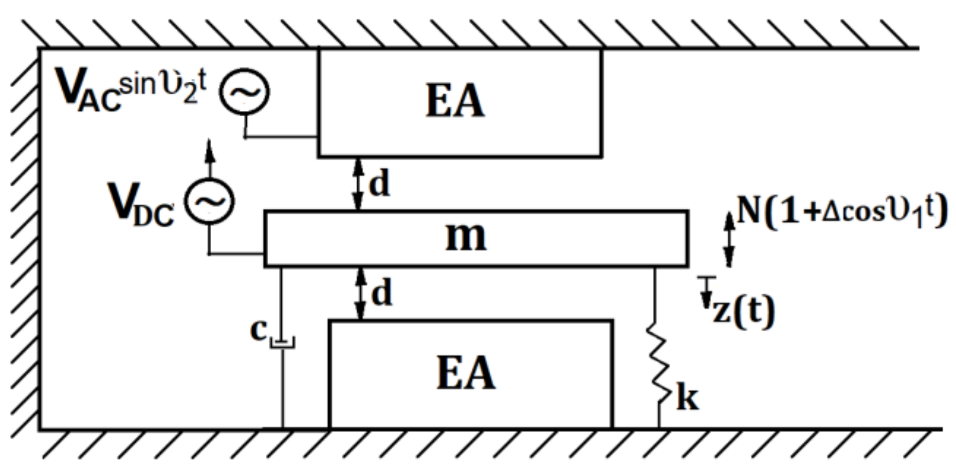
Henceforward we consider two symmetrical EA on the loss contact only on the frequency response of the Hertzian contact oscillator near the primary resonance. The model is depicted in Figure 1 and the governing equation can be written as [4,15,16]:
m z ¨ + c z ˙ + k z 3 / 2 = N ( 1 + Δ cos υ 1 t ) + F e m ,
where the dot denotes differentiation with respect to time t and z(t) is the normal displacement of the rigid mass m, c is the damping coefficient, k is the constant given by the Hertzian theory, N is the static normal load, ∆ is the amplitude, and ν1 is the frequency of the harmonic excitation load, and Fem is the electromagnetic force.
Within Equation (1) we took into consideration that the deformation between the solids in contact are elastic, the contact is maintained and the dry contact is equivalent with the linear viscous damping.
The vibrating beam of mass m is placed on z-axis between two fixed electrodes. The driving voltage Vbias + VACsinν2t is generated by the combined action of DC and AC voltage and sources on the resonator electrode. The interaction between the driving voltage and parallel plate causes the electromagnetic force
F e m = 1 2 C 0 ( d z ) 2 ( V b i a s + V A C sin υ 2 t ) 2 1 2 C 0 ( d + z ) 2 V b i a s , 2
in which C0 is the capacitance of the parallel-plate actuator, d is the initial gap width, and ν2 is the frequency.
Using Equation (2), the Equation (1) can be rewritten in the dimensionless form as
x + μ x + 1 + 2 x 3 3 / 2 = 1 + Δ cos ω τ + α 1 1 2 x 3 R 2 1 1 + 2 x 3 R 2 + β sin Ω τ 1 2 x 3 R 2 + γ ( 1 cos 2 Ω τ ) 1 2 x 3 R 2
where the prime denotes differentiation with respect to τ and
z s = N k 2 / 3 ; ω 0 2 = 3 k 2 m z s 3 / 2 ; z = z s 1 + 2 x 3 ; μ = C m ω 0 ; τ = ω 0 t ; d = z s ( 1 + R ) ; ω = υ 1 ω 0 ; υ 2 t = Ω τ ; Ω = υ 2 ω 0 ; α = C 0 V b i a s 2 2 k R 2 z s 5 / 2 ; β = C 0 V A C V b i a s k R 2 z s 5 / 2 ; γ = C 0 V A C 2 4 k R 2 z s 5 / 2
The following approximations are used:
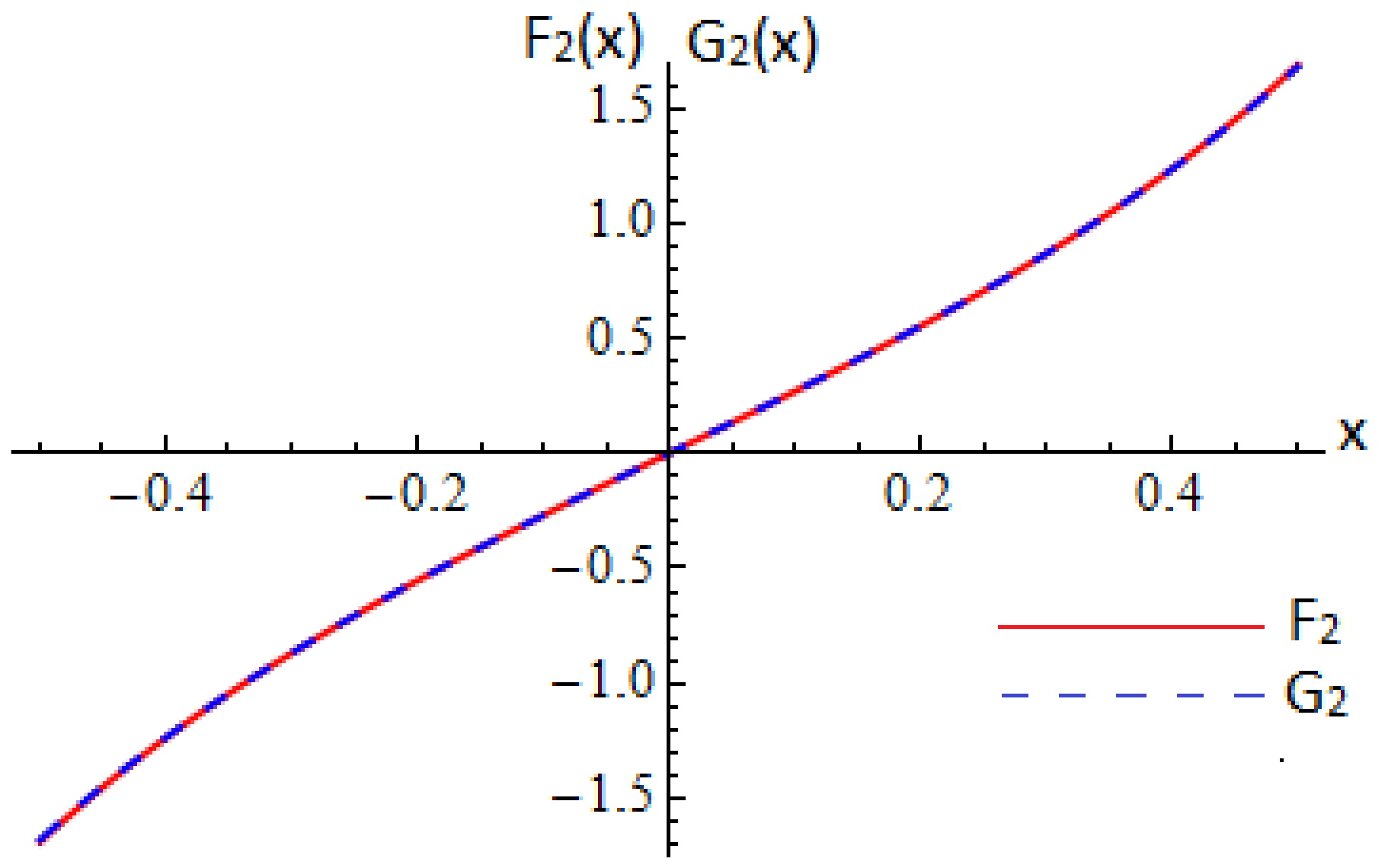
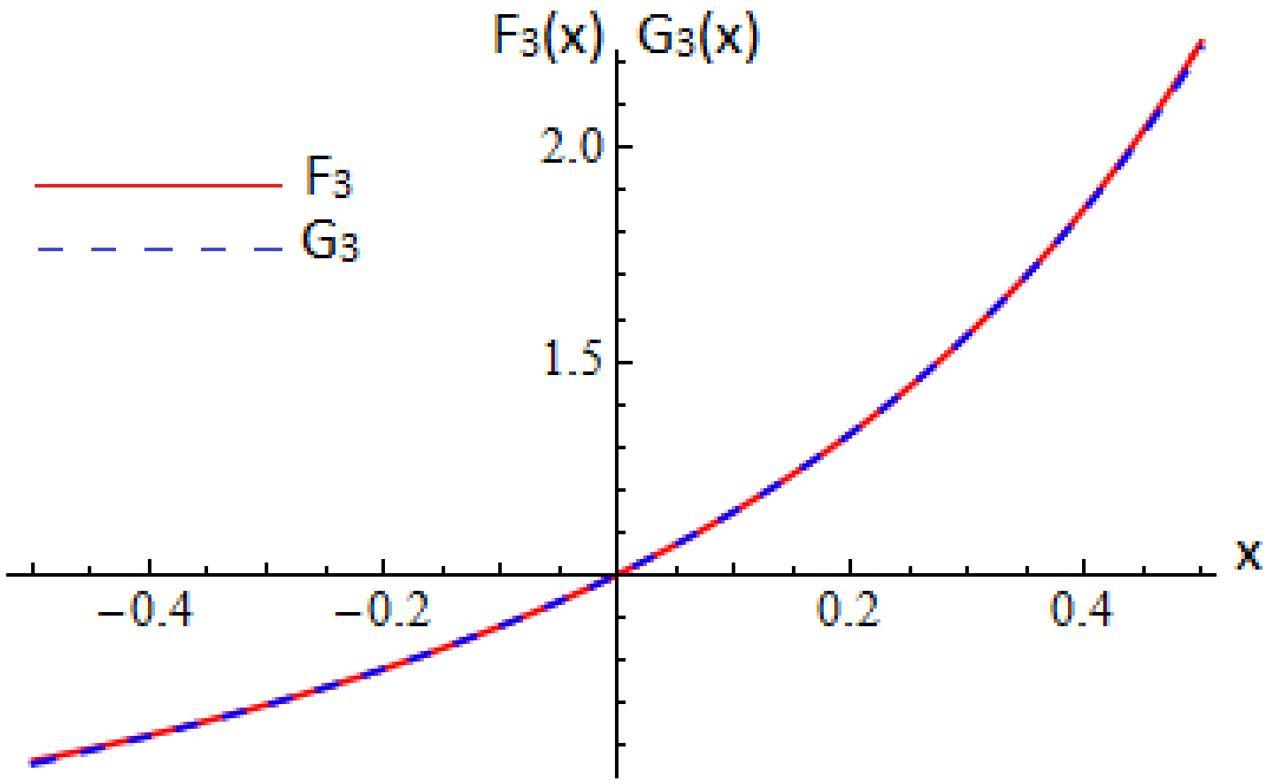
F 1 ( x ) = 1 + 2 x 3 R 3 / 2 1 + x R + x 2 6 R 2 x 3 54 R 3 + x 4 432 R 4 + x 5 1296 R 5 = G 1 ( x ) F 2 ( x ) = 1 1 2 x 3 R 2 1 1 + 2 x 3 R 2 8 x 3 R + 64 x 3 27 R 3 + 128 x 5 81 R 5 = G 2 ( x ) F 3 ( x ) = 1 1 2 x 3 R 2 1 + 4 x 3 R + 4 x 2 3 R 2 + 32 x 3 27 R 3 + 80 x 4 81 R 4 + 64 x 5 81 R 5 = G 3 ( x )
Figure 2, Figure 3 and Figure 4 depict the variations of Fi(x) and Gi(x), i = 1, 2, 3 for R = 1 on domain [−0.5–0.5]. The maximum errors of the approximations (5) are, respectively:
ε 1 = max x D F 1 ( x ) G 1 ( x ) = 1.3 10 6 ; ε 2 = max x D F 2 ( x ) G 2 ( x ) = 1.6 10 6 ε 3 = max x D F 3 ( x ) G 3 ( x ) = 7.9 10 6
In this way, Equation (3) can be rewritten in the form
x + μ x + a 1 x γ + a 2 x 2 + a 3 x 3 + a 4 x 4 + a 5 x 5 = Δ cos ω τ + + β 1 + 4 x 3 R + 4 x 2 3 R 2 + 32 x 3 27 R 3 + 80 x 4 81 R 4 + 64 x 5 81 R 5 sin Ω τ γ 1 + 4 x 3 R + 4 x 2 3 R 2 + 32 x 3 27 R 3 + 80 x 4 81 R 4 + 64 x 5 81 R 5 cos 2 Ω τ
where
a 1 = 1 8 α 3 R 4 γ 3 R ; a 2 = 1 6 4 γ 3 R 2 ; a 3 = 1 54 64 α 27 R 3 ; a 4 = 1 432 80 γ 81 R 5 ; a 5 = 1 1296 128 α 81 R 5 64 γ 81 R 5
It should be emphasized that in this paper no simplifying assumption is made as in other papers. For example, the amplitude of AC excitation voltage is much lower than the bias voltage [10,15,25]. In the present paper we consider only the primary resonance:
ω = a 1 + δ ε ; ε < < 1
in which δ is the detuning parameter from the primary resonance.
The initial conditions for the nonlinear differential Equation (7) are
x ( 0 ) = A ; x ( 0 ) = 0
It is clear that the Equation (7) with initial conditions (10) is a second order nonlinear differential equation with variable coefficients of the five order and therefore is very difficult to find an exact solution. In the following, for Equations (7) and (10) the OAFM is applied to study the nonlinear vibrations near the primary resonance.

3. Application of the OAFM

In order to apply OAFM [31,32,33,34,35,36], it is observed that the linear operator and the nonlinear operator corresponding to Equations (7) and (10) are, respectively:
L [ x ( τ ) ] = x + μ x + a 1 x
N [ x ( τ ) ] = γ + a 2 x 2 + a 3 x 3 + a 4 x 4 + a 5 x 5 Δ cos ω τ β 1 + 4 x 3 R + 4 x 2 3 R 2 + 32 x 3 27 R 3 + 80 x 4 81 R 4 + 64 x 5 81 R 5 sin Ω τ + γ 1 + 4 x 3 R + 4 x 2 3 R 2 + 32 x 3 27 R 3 + 80 x 4 81 R 4 + 64 x 5 81 R 5 cos 2 Ω τ
For Equations (7) and (10), the approximate analytical solution can be written as:
x ˜ ( τ ) = x 0 ( τ ) + x 1 ( τ , C 1 , C 2 , , C n )
where Ci, i = 1, 2, …, n are n parameters unknown at this moment, and n is an arbitrary positive integer fixed number. The initial approximation x0(τ) is determined from the following linear differential equation:
L [ x 0 ( τ ) ] = γ , x 0 ( 0 ) = A , x 0 ( 0 ) = 0
whose solution is
x 0 ( τ ) = γ a 1 + A γ a 1 e μ 2 τ ( cos p τ + μ 2 p sin p τ )
where p = ( ω δ ε ) 2 μ 2 / 4 . Inserting Equation (15) into Equation (12), after simple manipulations we obtain:
N [ x 0 ( τ ) ] = γ + a 2 A 2 2 p 2 + μ 2 4 p 2 e μ τ + a 4 A 4 3 μ 4 + 22 μ 2 p 2 + 12 p 4 32 p 4 e 2 μ τ Δ cos ω τ + + a 3 A 3 3 ( 4 p 2 + μ 2 ) 16 p 2 e 3 μ 2 τ + a 5 A 5 5 8 + 5 μ 2 16 p 2 + 5 μ 4 128 p 4 e 5 μ 2 τ cos p τ + a 3 A 3 3 μ ( 16 p 2 μ 2 ) 32 p 3 e μ τ + a 5 A 5 5 μ 16 p + 5 μ 3 32 p 3 + 5 μ 5 256 p 5 e 5 μ 2 τ sin p τ + a 2 A 2 2 p 2 μ 2 4 p 2 e μ τ + a 4 A 4 4 p 4 μ 4 8 p 4 e 2 μ τ cos 2 p τ + + a 2 A 2 μ 2 p e μ τ + a 4 A 4 μ ( 2 p 2 + μ 2 ) 4 p 3 e 2 μ τ sin 2 p τ + a 3 A 3 4 p 2 3 μ 2 16 p 2 e 3 μ 2 τ + a 5 5 16 5 μ 2 32 p 2 15 μ 4 256 p 4 e 5 μ 2 τ cos 3 p τ + a 3 A 3 μ ( 12 p 2 μ 2 ) 32 p 3 e 3 μ 2 τ + a 5 A 5 15 μ 32 p + 5 μ 3 64 p 3 5 μ 5 512 p 5 e 5 μ 2 τ sin 3 p τ + + a 4 A 4 μ 4 8 μ 2 p 2 + 4 p 4 32 p 4 e 2 μ τ cos 4 p τ + μ ( 2 p 2 μ 2 ) 2 p 3 e 2 μ τ sin 4 p τ + + a 5 A 5 e 5 μ 2 τ 1 16 + 5 μ 2 32 p 2 + 5 μ 4 256 p 4 cos 5 p τ + 5 μ 32 p 5 μ 3 64 p 3 + μ 5 512 p 5 sin 5 p τ + ( β sin Ω τ γ cos 2 Ω τ ) 1 + 4 A 2 ( μ 2 + 2 p 2 ) 12 Ω 2 p 2 e μ τ + 5 A 4 ( 3 μ 4 + 22 μ 2 p 2 + 12 p 4 ) 162 R 4 p 4 e 2 μ τ + 4 A 3 Ω e μ 2 τ + 2 A 3 ( 4 p 2 + μ 2 ) 9 R 5 p 2 e 3 μ 2 τ + + A 5 ( 80 p 4 + 40 p 2 μ 2 + 5 μ 4 ) 162 R 5 p 4 e 5 μ 2 τ cos p τ + 2 A μ 3 R p e μ 2 τ + A 3 μ ( 16 p 2 + μ 2 ) 9 R 3 p 3 e 3 μ 2 τ +
+ A 5 ( 80 μ p 4 + 40 μ 3 p 2 + 5 μ 5 ) 324 R 5 p 5 e 5 μ 2 τ sin p τ + A 2 ( 2 p 2 μ 2 ) 3 R 2 p 2 e μ τ + 10 A 4 ( 4 p 4 μ 4 ) 81 Ω 4 p 4 e 2 μ τ cos 2 p t + + 2 A 2 μ 3 R 2 p e μ τ + 20 A 4 ( A 3 2 μ p 2 ) 81 R 4 p 3 e 2 μ τ sin 2 p τ + 2 A 3 ( 4 p 2 3 μ 2 ) 27 R 3 p 3 e 3 μ 2 τ + + A 5 ( 240 μ p 4 40 μ 2 p 2 + 5 μ 4 ) 324 R 3 p 4 e 5 μ 2 τ cos 3 p τ + A 3 ( 12 μ p 2 μ 3 ) 27 R 3 p 3 e 3 μ 2 τ + + A 5 ( 240 μ p 4 + 40 μ 3 p 2 5 μ 2 ) 648 R 5 p 5 e 5 μ 2 τ sin 3 p τ + 5 A 4 ( μ 4 8 μ 2 p 2 + 4 p 4 ) e 2 μ τ 162 R 4 p 4 cos 4 p τ + + 40 A 4 ( 2 μ p 2 μ 3 ) e 2 μ τ 81 R 4 p 3 sin 4 p τ + A 5 ( 16 p 4 + 4 p 2 μ 2 + 5 μ 4 ) e 5 μ 2 τ 324 R 5 p 4 cos 5 p τ + + A 5 ( 80 μ p 4 40 μ 3 p 2 + μ 3 ) e 5 μ 2 τ 648 R 5 p 5 sin 5 p τ
To obtain the first approximation x1(τ,C1,C2,…,Cn), we choose this function in the form:
x 1 ( τ , C 1 , C 2 , , C n ) = x 10 ( τ , C 1 , C 2 , , C n ) + x 20 ( τ , C 1 , C 2 , , C n )
where x10(τ,Ci) can be obtained by using Equations (15) and (16) in the form:
L [ x 10 ( τ , C i ) ] = G j ( e k μ τ , cos p τ , sin p τ , cos 3 p τ , sin 3 p τ , )
in which Gj are combinations of the functions which appear into Equations (15) and (16). These auxiliary functions Gj are not unique. For example, the auxiliary function Gj can be of the form:
G 1 ( e k μ τ , cos p τ , sin p τ , cos 3 p τ , sin 3 p τ ) = e μ τ ( C 1 cos p τ + C 2 sin p τ + C 3 cos 3 p τ + C 4 sin 3 p τ )
or
G 2 ( e k μ τ , cos p τ , sin p τ , cos 3 p τ , sin 3 p τ ) = e μ 2 τ ( C 1 cos p τ + C 2 sin p τ + C 3 sin 3 p τ )
or
G 3 ( e k μ τ , cos p τ , sin p τ , cos 3 p τ , sin 3 p τ ) = e μ 3 τ ( C 1 cos p τ + C 2 sin p τ + C 3 cos 3 p τ + C 4 cos 5 p τ + + C 5 sin 3 p τ + C 6 sin 3 p τ )
and so on. The initial condition for the first iteration are obtained from Equations (10) and (14):
x 1 ( 0 ) = 0 , x 1 ( 0 ) = 0
Having in view only Equations (19) and (22), the function x10 can be obtained from the linear differential equation:
L [ x 10 ( τ , C i ) ] = e μ τ ( C 1 cos p τ + C 2 sin p τ + C 3 cos 3 p τ + C 4 sin 3 p τ ) , x 1 ( 0 ) = x 1 ( 0 ) = 0
The solution of the last equation is
x 10 ( τ , C i ) = M 1 ( e μ τ sin p τ e μ τ 2 sin p τ ) + M 2 e μ t cos p τ + e μ τ 2 ( μ 2 p sin p τ cos p τ ) + + M 3 e μ t cos 3 p τ e μ τ 2 ( cos p τ μ 2 p sin p τ ) + M 4 e μ t sin 3 p τ 3 e μ τ 2 sin p τ
where
M 1 = μ p C 1 + ( a 1 p 2 ) C 2 μ 2 p 2 + ( a 1 p 2 ) 2 ; M 2 = ( a 1 p 2 ) C 1 μ p C 2 μ 2 p 2 + ( a 1 p 2 ) 2 ; M 3 = ( a 1 9 p 2 ) C 3 3 μ p C 4 9 μ 2 p 2 + ( a 1 9 p 2 ) 2 M 4 = 3 μ p C 3 + ( a 1 9 p 2 ) C 4 9 μ 2 p 2 + ( a 1 9 p 2 ) 2
We have a great freedom to choose the function x20 from Equation (17):
x 20 ( τ , C i ) = M 1 ( e μ τ 35 e μ τ 30 ) sin p τ M 1 ( e μ t e μ τ 2 ) sin p τ
or
x 20 ( τ , C i ) = M 4 ( e μ τ 35 e μ τ 30 ) sin p τ M 4 ( e μ t sin p τ 3 e μ τ 2 sin p τ )
or
x 20 ( τ , C i ) = M 1 ( e μ τ 15 e μ τ 10 ) sin p τ M 1 ( e μ t e μ τ 2 ) sin p τ
and so on.
If we choose the expression (26) for the function x20(τ,Ci), then the first approximation is obtained from Equations (17), (24) and (26):
x 1 ( τ , C 1 , C 2 , C 3 , C 4 ) = M 1 ( e μ τ 35 sin p τ e μ τ 30 sin p τ ) + M 2 e μ t cos p τ + e μ τ 2 μ 2 p sin p τ cos p τ + + M 3 e μ t cos 3 p τ e μ τ 2 ( cos p τ μ 2 p sin p τ ) + M 4 ( e μ t sin 3 p τ 3 e μ τ 2 sin p τ )
The approximate solution of clamped, forced oscillator can be obtained from Equations (13), (15) and (29):
x ˜ ( τ , C 1 , C 2 , C 3 , C 4 ) = γ a 1 + A γ a 1 e μ τ 2 ( cos p τ + μ 2 p sin p τ ) + M 1 ( e μ τ 35 sin p τ e μ τ 30 sin p τ ) + + M 2 e μ t cos p τ + e μ τ 2 μ 2 p sin p τ cos p τ + M 3 e μ t cos 3 p τ e μ τ 2 ( cos p τ μ 2 p sin p τ ) + + M 4 ( e μ t sin 3 p τ 3 e μ τ 2 sin p τ )
where the coefficients Mi, i = 1, 2, 3, 4 are given by Equation (25).
It is known that the damped solution (30) is valid on a certain domain D = [0,τ*]. For the steady-state solution, valid for τ > τ*, the linear and nonlinear operators are, respectively:
L [ x ( τ ) ] = x + a 1 x
N [ x ( τ ) ] = γ + a 2 x 2 + a 3 x 3 + a 4 x 4 + a 5 x 5 Δ cos ω τ β 1 + 4 x 3 R + 4 x 2 3 R 2 + 32 x 3 27 R 3 + 80 x 4 81 R 4 + 64 x 5 81 R 5 sin Ω τ + γ 1 + 4 x 3 R + 4 x 2 3 R 2 + 32 x 3 27 R 3 + 80 x 4 81 R 4 + 64 x 5 81 R 5 cos 2 Ω τ
The initial approximation is obtained from the linear differential equation:
L [ x 0 ( τ ) ] = 0 , x 0 ( τ * ) = x ˜ ( τ * ) , x 0 ( τ * ) = x ˜ ( τ * )
where x ˜ τ * and x ˜ τ * are obtained from Equation (30), so as to ensure the continuity of the solution.
The solution of Equation (32) is:
x 0 ( τ ) = x ˜ ( τ * ) cos p * ( τ τ * ) + x ˜ ( τ * ) sin p * ( τ τ * )
The first approximation x1(τ) can be obtained similarly to Equation (23):
L [ x 1 ( τ ) ] = C 5 sin 3 p * ( τ τ * ) + C 6 sin 5 p * ( τ τ * ) + C 7 sin 7 p * ( τ τ * ) , x 1 ( τ * ) = x 1 ( τ * ) = 0
from which
x 1 ( τ ) = C 5 [ 3 sin p * ( τ τ * ) sin 3 p * ( τ τ * ) ] + C 6 [ 5 sin p * ( τ τ * ) sin 5 p * ( τ τ * ) ] + + C 7 [ 7 sin p * ( τ τ * ) sin 7 p * ( τ τ * ) ]
The steady-state solution of Equations (7) and (10) is obtained from Equations (13), (33) and (35):
N [ x ( τ ) ] = γ + a 2 x 2 + a 3 x 3 + a 4 x 4 + a 5 x 5 Δ cos ω τ β 1 + 4 x 3 R + 4 x 2 3 R 2 + 32 x 3 27 R 3 + 80 x 4 81 R 4 + 64 x 5 81 R 5 sin Ω τ + γ 1 + 4 x 3 R + 4 x 2 3 R 2 + 32 x 3 27 R 3 + 80 x 4 81 R 4 + 64 x 5 81 R 5 cos 2 Ω τ

4. Numerical Example

The efficiency of our procedure can be proved considering the following particular case, characterized by the following parameters:
A = 0.04, μ = 0.1, ∆ = 0.0007, α = 0.001, β = 0.0001, γ = 0.0002, δ = 0.02, ε = 0.01, R = 1.
From the above procedure, the optimal values of the convergence-control parameters are determined by minimizing the residual of the governing equation:
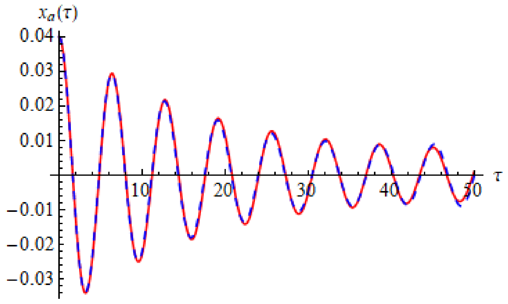
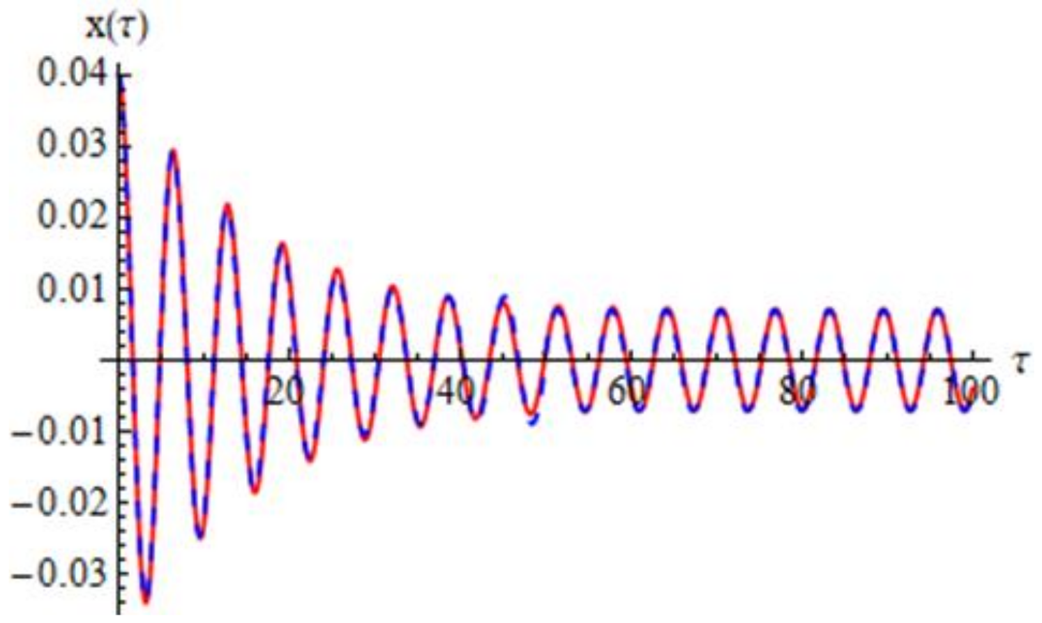
C 1 = 0 . 030429 ,   C 2 = 0 . 00073852 ,   C 3 = - 0 . 000338155 ,   C 4 = 0 . 000342986 , τ * = 50
The Figure 5 shows the comparison between approximate solution (30) of nonlinear problem (7) and (10) and numerical solution obtained by means of a fourth-order Runge-Kutta approach for τ = [0,50].
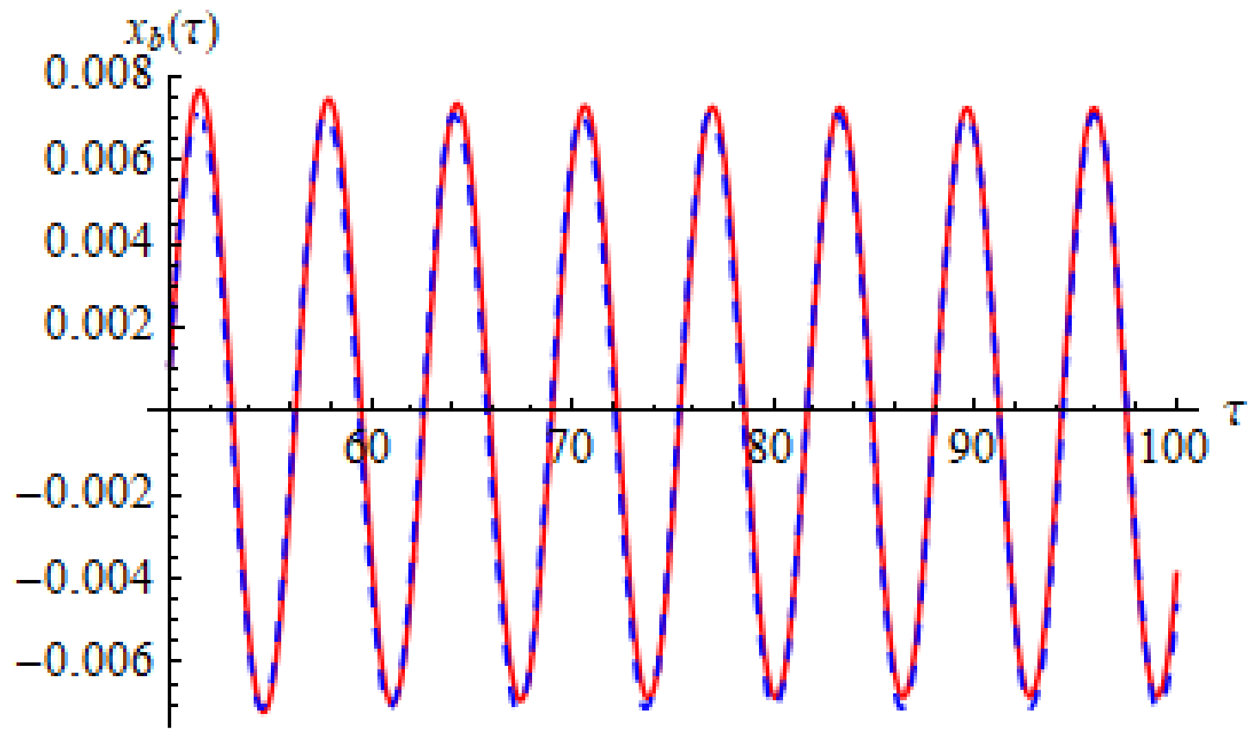
For the steady-state solution (t > 50) the optimal values of the convergence-control parameters are
C 5 = - 0 . 000003211 ,   C 6 = 0 . 000016621 ,   C 7 = 0 . 0000563803 , τ * = 50 , p * = 0 . 988
and the comparison between the corresponding approximate solution and numerical integration results is presented in Figure 6.
From Figure 7, it can be seen that the two solutions for τ < 50 and τ > 50 obtained using the proposed technique are nearly identical with that obtained through numerical integration and this excellent agreement validates the proposed approach and the obtained results.

5. Analysis of the Stability of Steady-State Motion for the Primary Resonance

In this section we use a perturbation method to investigate the stability of the steady-state motion. For this aim we use the transformation [37]
ξ = ω τ ; η = ε τ ; ω = a 1 + δ ε
In order to substitute this transformation into Equation (7), we need expressions of the first and second derivatives of variable x with respect to τ. We obtain
d x d τ = x ξ d ξ d τ + x η d η d τ = ω x ξ + ε x η = a 1 + δ ε x ξ + ε x η d 2 x d τ 2 = ω 2 2 x ξ 2 + 2 ω ε 2 x ξ η + ε 2 2 x η 2 = a 1 + δ ε 2 2 x ξ 2 + 2 a 1 + δ ε ε 2 x ξ η + ε 2 2 x η 2
Expanding x in power series, one can get:
x ( ξ , η ) = X ( ξ , η ) + ε X 1 ( ξ , η ) +
Substituting Equation (41) into Equation (7) it holds that
X + ε X 1 + μ ( X + ε X 1 ) + a 1 ( X + ε X 1 ) γ + a 2 ( X 2 + 2 ε X X 1 + ε 2 X 2 ) + a 3 ( X 3 + 3 ε X X 1 2 + 3 ε 2 X X 1 2 + + ε 3 X 1 3 ) + a 4 ( X 4 + 4 ε X 3 X 1 + 6 ε 2 X 2 X 1 2 + 4 ε 3 X X 1 3 + ε 4 X 4 ) + a 5 ( X 5 + 5 ε X 4 X 1 + 10 ε 2 X 3 X 1 2 + + 10 ε 3 X 2 X 1 3 + 5 ε 4 X X 1 4 + ε 5 X 5 ) Δ cos ω τ ( β sin Ω τ γ cos 2 Ω τ ) 1 + 4 ( X + ε X 1 ) 3 R + + 4 ( X 2 + 2 ε X X 1 + ε 2 X 1 2 ) 3 R 2 + 32 ( X 3 + 3 ε 2 X 2 X 1 + 3 ε 2 X X 1 2 + ε 3 X 1 3 ) 27 R 3 + + 80 ( X 4 + 4 ε X 3 X 1 + 6 ε 2 X 2 X 1 2 + 4 ε 3 X X 1 3 + ε 4 X 1 4 ) 81 R 4 + + 64 ( X 5 + 5 ε X 4 X 1 + 10 ε 2 X 3 X 1 2 + 10 ε 3 X 2 X 1 3 + 5 ε 4 X X 1 4 + ε 5 X 1 5 ) 81 R 5 = 0
Averaging Equation (42) we obtain
X + μ X + a 1 X γ + a 2 ( X 2 + ε 2 < X 1 2 > ) + a 3 ( X 3 + 3 ε 2 X < X 1 2 > ) + a 4 ( X 4 + 6 ε 2 X 2 < X 1 2 > + + ε 4 < X 1 4 > + a 5 ( X 5 + 10 ε 2 X 3 < X 1 2 > + 5 ε 4 X < X 1 4 > ) Δ cos ω τ = 0
Subtracting Equations (42) and (43) yields
ε X 1 + ε μ X 1 + ε a 1 X 1 + ε a 1 X 1 + a 2 [ 2 ε X X 1 + ε 2 ( X 1 2 < X 1 2 > ) + a 3 ( 3 ε X 2 X 1 + 3 ε 2 X ( X 1 2 < X 1 2 > ) + + ε 3 X 1 3 ] + a 4 [ 4 ε X 3 X 1 + 6 ε 2 X 2 2 ( X 1 2 < X 1 2 > ) + 4 ε 3 X X 1 3 + ε 4 ( X 1 4 < X 1 4 > ) ] + a 5 [ 5 ε X 4 X 1 + + 10 ε 2 X 2 ( X 1 2 < X 1 2 > ) + 10 ε 3 X 2 X 1 3 + 5 ε 4 X ( X 1 4 < X 1 4 > ) + ε 5 X 1 5 ] ( β sin Ω τ γ cos 2 Ω τ ) 4 ( X + ε X 1 ) 3 R + 4 ( X 2 + 2 ε X X 1 + ε 2 X 1 2 ) 3 R 2 + 32 ( X 3 + 3 ε 2 X 2 X 1 + 3 ε 2 X X 1 2 + ε 3 X 1 3 ) 27 R 3 + + 80 ( X 4 + 4 ε X 3 X 1 + 6 ε 2 X 2 X 1 2 + 4 ε 3 X X 1 3 + ε 4 X 1 4 ) 81 R 4 + + 64 ( X 5 + 5 ε X 4 X 1 + 10 ε 2 X 3 X 1 2 + 10 ε 3 X 2 X 1 3 + 5 ε 4 X X 1 4 + ε 5 X 1 5 ) 81 R 5 ( β sin Ω τ γ cos 2 Ω τ ) = 0
Using the so-called inertial approximation [37], i.e., all terms of Equation (44) can be ignored, except the first and the last terms, such that:
ε X 1 ( β sin Ω τ γ cos Ω τ ) = 0
from which we have:
ε X 1 = β Ω 2 sin Ω τ + γ 4 Ω 2 cos 2 Ω τ
Inserting Equation (46) into Equation (43) and taking into account the following identities:
< ε X 1 2 > = 1 Ω 4 2 π 0 2 π / Ω ( β sin Ω τ γ 4 cos 2 Ω τ ) d τ = γ 2 + 16 β 2 32 Ω 4
< ε 4 X 1 4 > = 1 Ω 8 2 π 0 2 π / Ω ( β sin Ω τ γ 4 cos 2 Ω τ ) d τ = 3 ( 4 λ 4 + γ 2 β 2 + 4 β 4 ) 32 Ω 8
We find the approximate equation for the variable X in the form
X + μ X + A 1 X + A 2 X 2 + A 3 X 3 + A 4 X 4 + A 5 X 5 + Γ Δ cos ω τ = 0
in which
A 1 = a 1 + 3 ( γ 2 + 16 β 2 ) 32 Ω 4 a 3 + 15 ( 4 γ 4 + γ 2 β 2 + 4 β 2 ) 32 Ω 8 a 5 ; A 2 = a 2 + 3 ( γ 2 + 16 β 2 ) 16 Ω 4 a 4 ; A 3 = a 3 + 5 ( γ 2 + 16 β 2 ) 16 Ω 4 a 5 ; A 4 = a 4 ; A 5 = a 5 ; Γ = γ + γ 2 + 16 β 2 32 Ω 4 a 2 + 3 ( 4 γ 4 + γ 2 β 2 + 4 β 4 ) 32 Ω 4 a 4
Now, introducing a bookkeeping parameter ε ¯ and scaling μ = ε ¯ μ , A i = ε ¯ A i ,   i = 1 , 2 , , 5 , with notation
X ( ξ , μ ) = u ( ξ , μ ) + ε ¯ v ( ξ , μ )
and then taking into consideration Equation (40), Equation (49) can be rewritten as
( a 1 + δ ε ¯ ) 2 u ξ 2 + ε ¯ 2 v ξ 2 + 2 ( a 1 + δ ε ¯ ) ε ¯ 2 u ξ η + ε ¯ 2 v ξ η + ε ¯ 2 2 u ξ 2 + ε ¯ 2 v η 2 + + ( a 1 + δ ε ¯ ) 2 u ξ 2 + ε ¯ v η + ε ¯ u ξ + ε ¯ v η + ε ¯ A 1 ( u + ε ¯ v ) + ε ¯ A 2 ( u + ε ¯ v ) 2 + ε ¯ A 3 ( u + ε ¯ v ) 3 + + ε ¯ A 4 ( u + ε ¯ v ) 4 + ε ¯ ( u + ε ¯ v ) 3 + Γ Δ cos ξ = 0
We seek a solution of Equation (52), equating the terms of same power of ε ¯ :
a 1 2 u ξ 2 + A 1 u + Γ = 0
a 1 2 v ξ 2 + A 1 v + 2 a 1 δ 2 u ξ 2 + 2 a 1 2 u ξ η + μ a 1 u ξ + A 1 u 2 + A 3 u 3 + A 4 u 4 + A 5 u 5 Δ cos ξ = 0
The solution of Equation (53) is of the form:
u ( ξ , η ) = A ( η ) cos ξ + B ( η ) sin ξ Γ A 1
Substituting Equation (55) into Equation (54) and avoiding secular terms, we obtain after some manipulations:
2 d A d η + μ A + 2 δ B 3 A 3 a 1 B ( A 2 + B 2 ) 5 A 5 a 1 B ( A 2 + B 2 ) B 2 Γ A 2 a 1 1.5 + 3 Γ 2 A 3 a 1 2.5 + 4 Γ 3 A 4 a 1 3.5 + 5 Γ 4 A 5 a 1 4.5 = 0
2 d B d η + μ B 2 δ A + 3 A 3 a 1 A ( A 2 + B 2 ) + 5 A 5 a 1 A ( A 2 + B 2 ) + A 2 Γ A 2 a 1 1.5 + 3 Γ 2 A 3 a 1 2.5 + 4 Γ 3 A 4 a 1 3.5 + 5 Γ 4 A 5 a 1 4.5 = Δ a 1
Equilibrium points of Equations (56) and (57), correspond to periodic motion such that d A d η = d B d η = 0 .
Using the notation:
θ = 2 Γ A 2 a 1 1.5 + 3 Γ 2 A 3 a 1 2.5 + 4 Γ 3 A 4 a 1 3.5 + 5 Γ 4 A 5 a 1 4.5
from Equations (56) and (57) we obtain
μ A + ( 2 δ θ ) B 3 A 3 B ( A 2 + B 2 ) a 1 5 a 5 B ( A 2 + B 2 ) 2 a 1 = 0
( θ 2 δ ) A + μ B + 3 A 3 A ( A 2 + B 2 ) a 1 + 5 a 5 A ( A 2 + B 2 ) 2 a 1 = Δ a 1
From algebraic Equations (59) and (60) one can get
A = Δ W μ a 1 ( 1 + W 2 ) , B = Δ W 2 μ a 1 ( 1 + W 2 )
where 
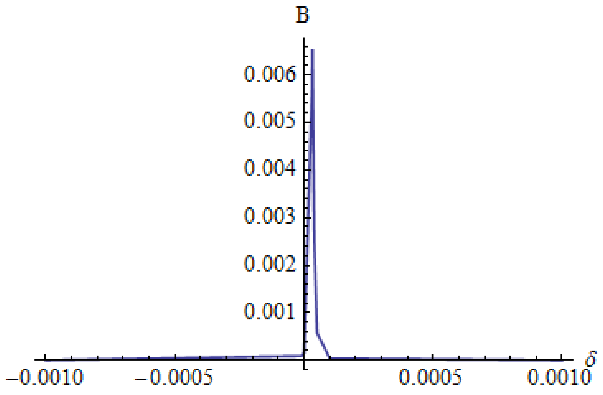
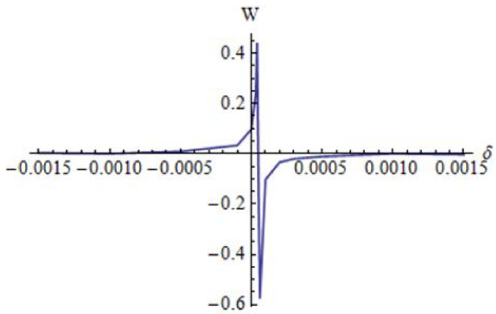
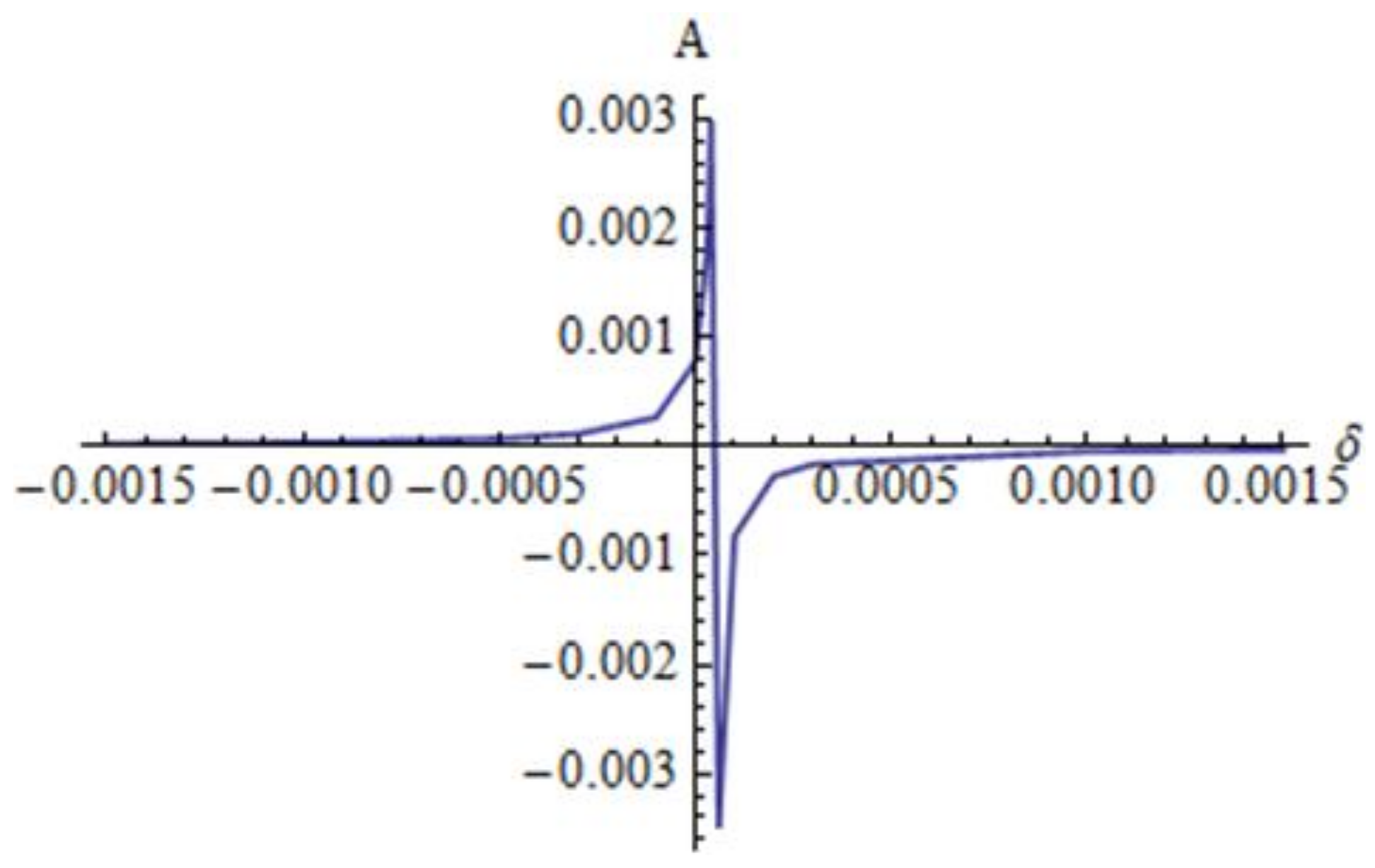
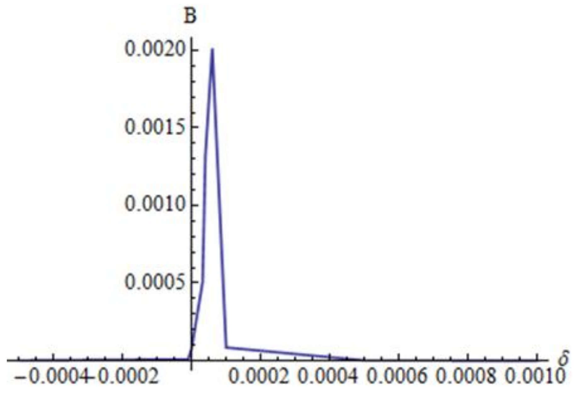
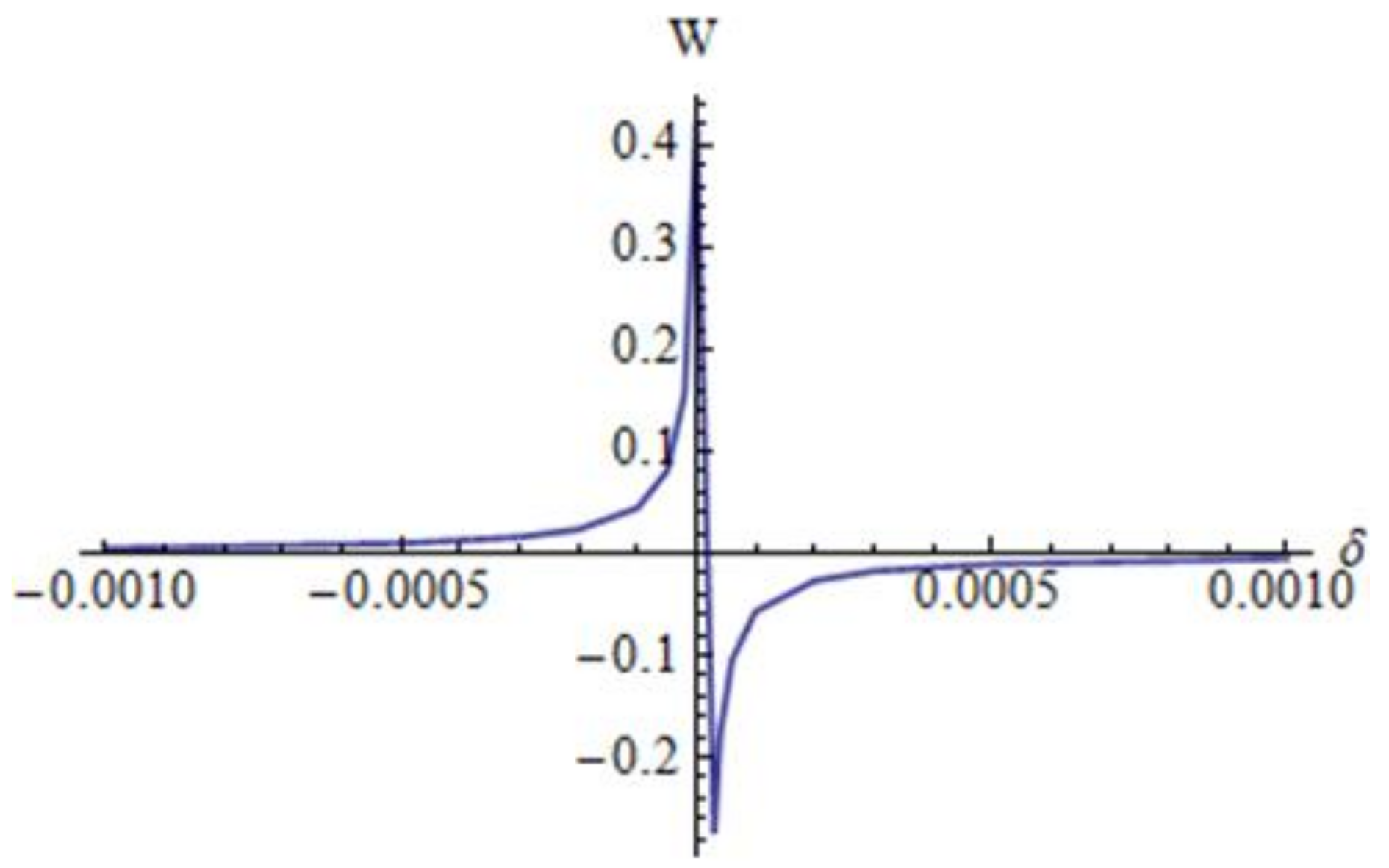
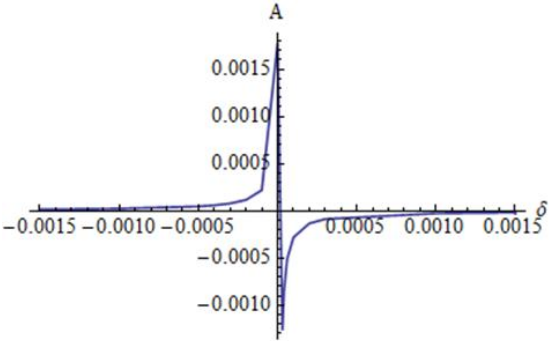
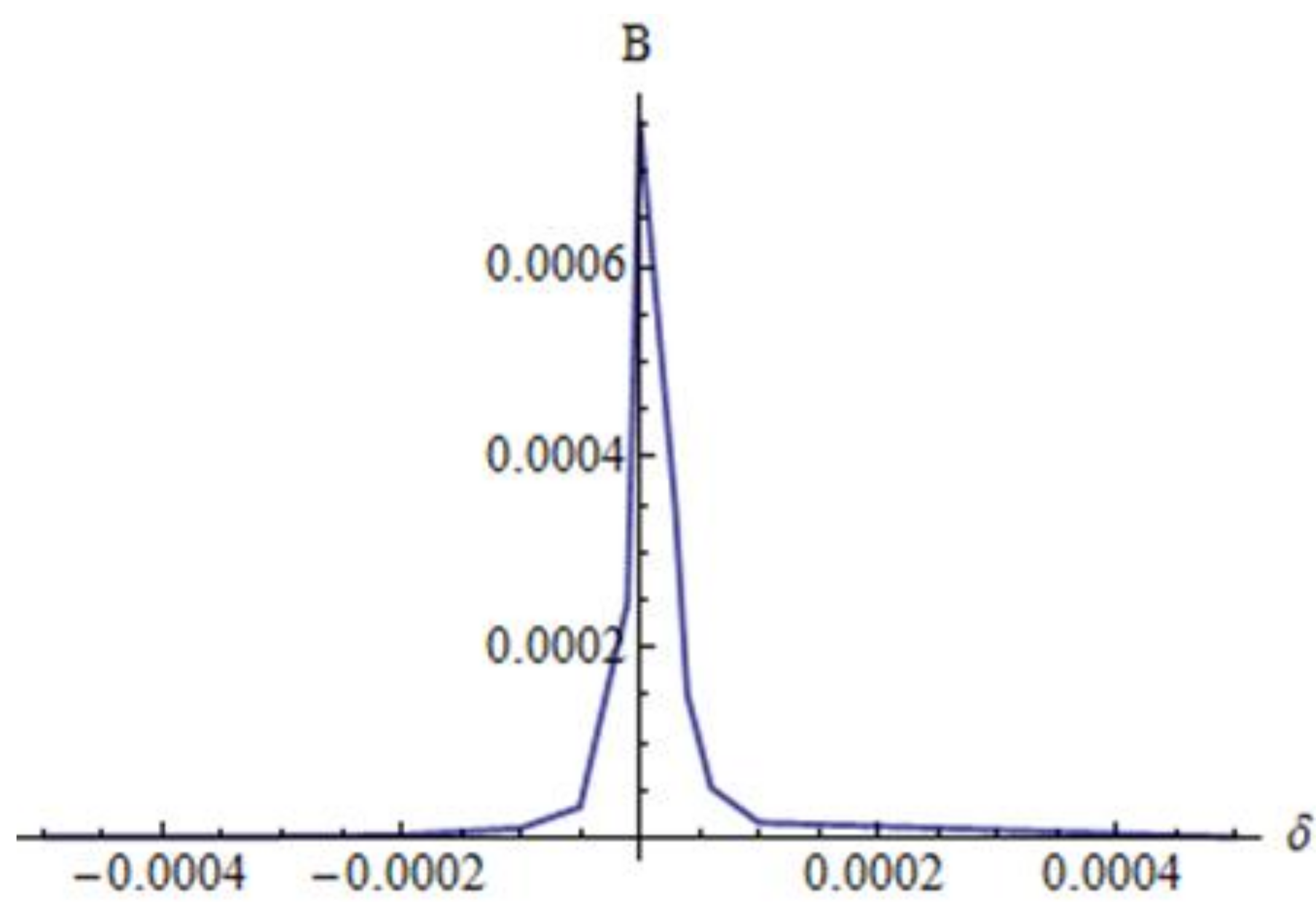
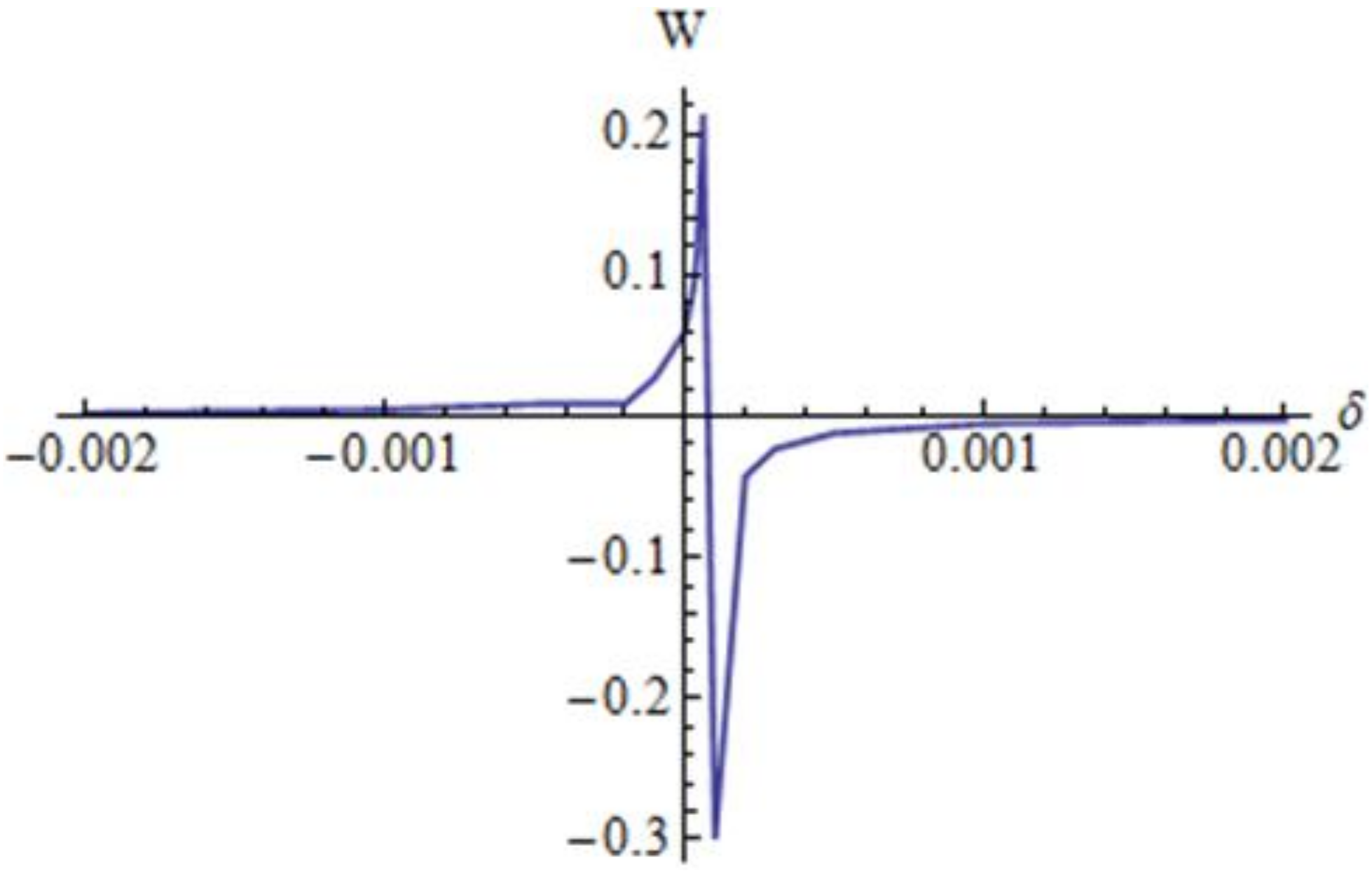
W is obtained from the following nonlinear equation:
W 2 1 + W 2 2 + 3 a 1 A 3 μ 2 5 A 5 Δ 2 W 2 1 + W 2 + ( θ 2 δ ) a 1 2.5 5 A 5 Δ 4 μ 5 a 1 1.5 5 A 5 Δ 4 W = 0
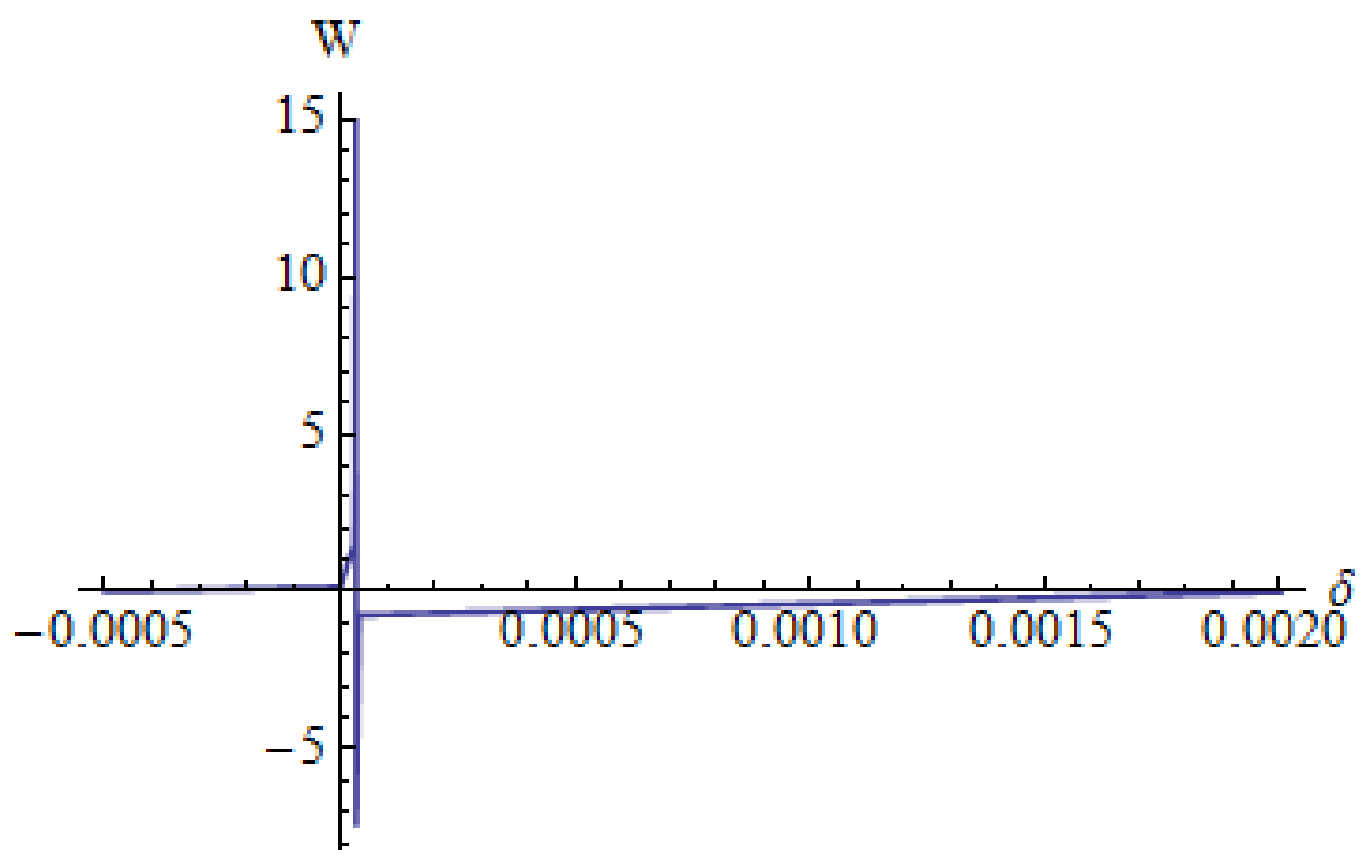
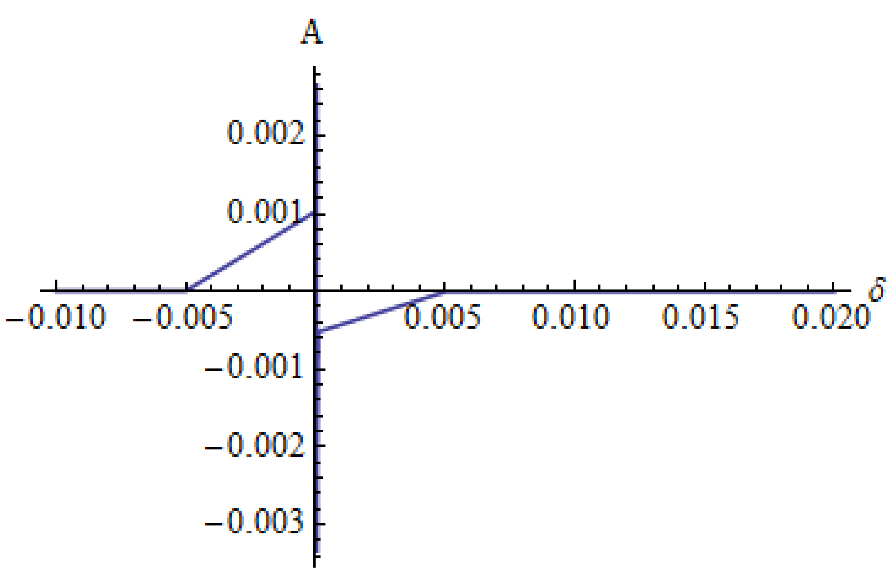
From Equation (62) it can be obtained 
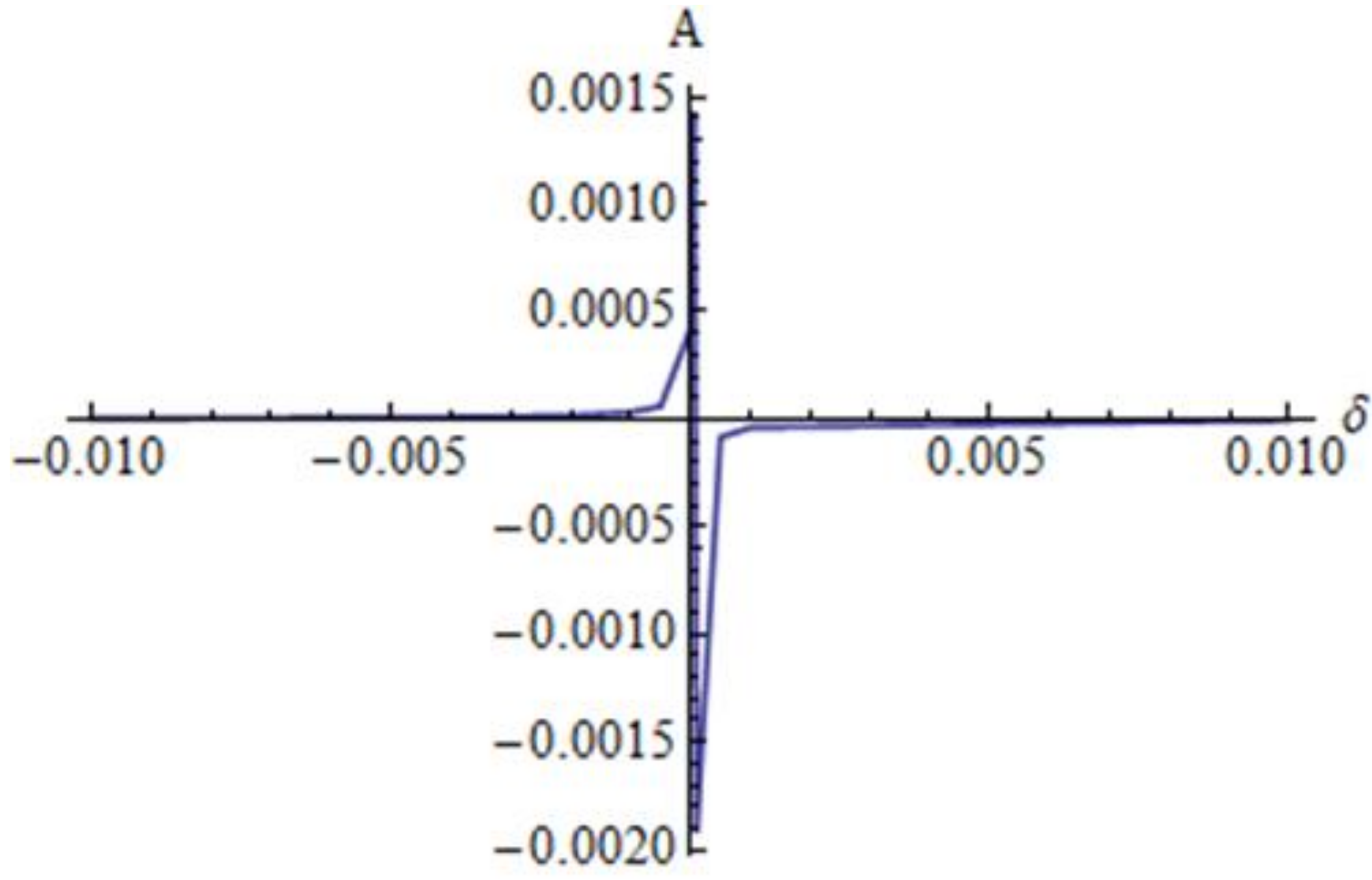
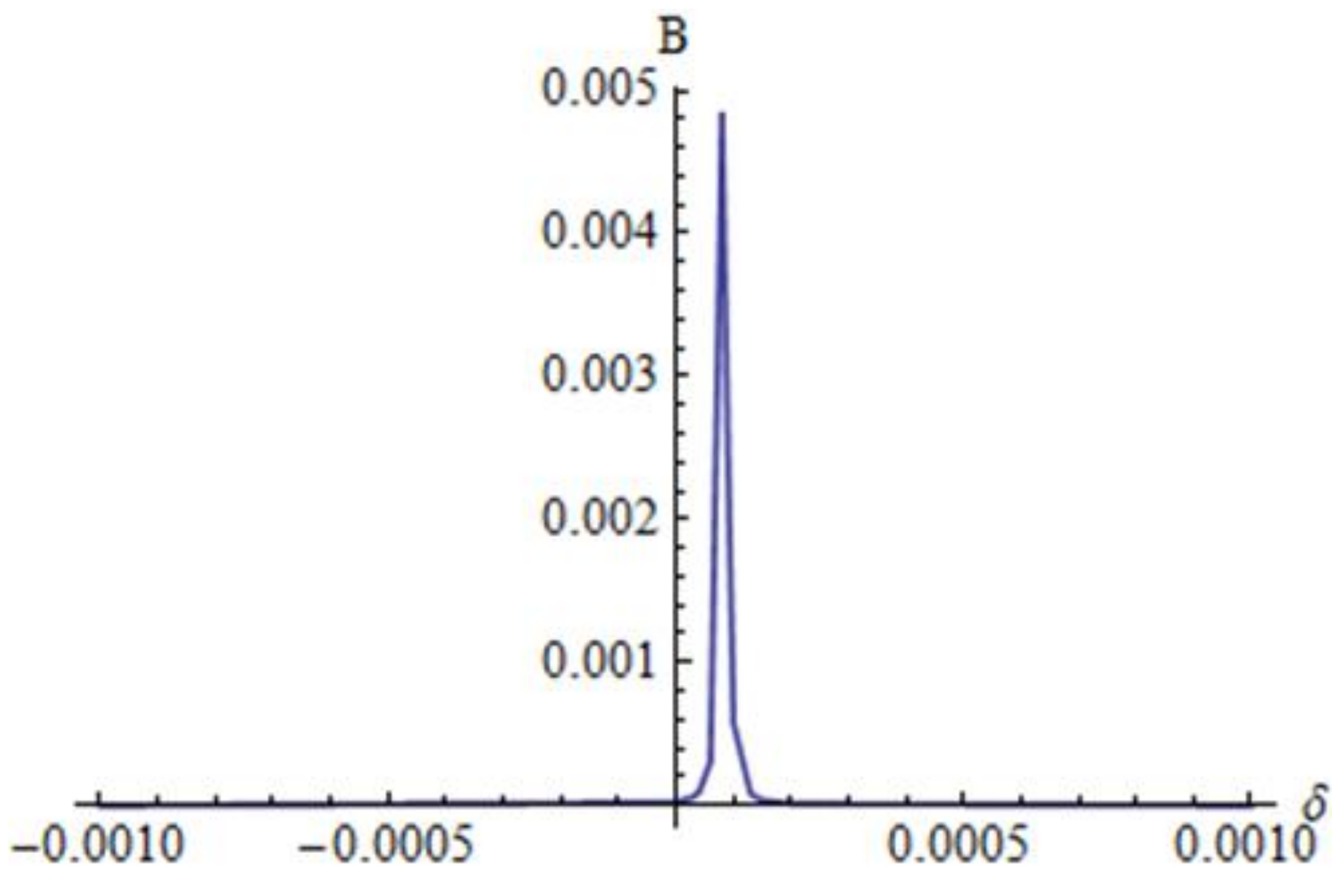
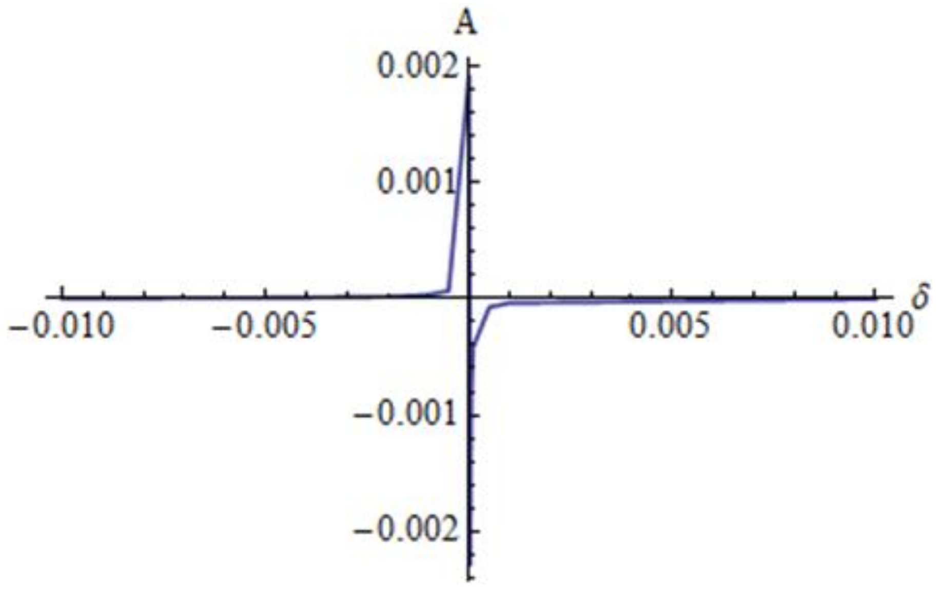
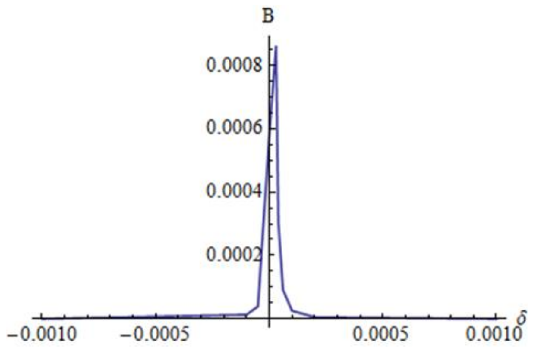
W as a function of δ. In this way the values of the equilibrium points A and B are known. For example, Figure 8, Figure 9 and Figure 10 depict the function W from (62) and the equilibrium points A and B from Equation (61) in the particular case a1 = 1; a2 = 1/6; a3 = −1/54; a4 = 1/432; a5 = 1/1296; γ = 0.0002.
In Figure 8, Figure 9, Figure 10, Figure 11, Figure 12, Figure 13, Figure 14, Figure 15, Figure 16, Figure 17, Figure 18, Figure 19, Figure 20, Figure 21 and Figure 22 it can be observed the influence of some key parameters on the system stability. From Figure 12, Figure 13, Figure 15 and Figure 16 it is observed that in the neighborhood of the origin, the amplitudes of A and B decrease with the increases of the parameter a1. In the outside of the neighborhood of the origin, the amplitudes of A and B are very little influenced by the parameter a1. The same conclusions can be drawn concerning the influence of the parameter γ: the amplitudes of A and B decrease with the increases of the parameter γ in the neighborhood of the origin, but outside of the neighborhood of the origin, the amplitudes of A and B are very little influenced by γ.
In order to determine stability of the equilibria, we will construct the Jacobian matrix, obtained from Equations (59), (61) and (62):
[ J ] = a 11 a 12 a 21 a 22
where
a 11 = A d A d η ; a 12 = B d A d η ; a 21 = A d B d η ; a 22 = B d B d η
and therefore
[ J ] = μ 2 + 3 A 3 Δ 2 W 3 a 1 1.5 μ 2 ( 1 + W 2 ) + 10 A 5 Δ 4 W 4 a 1 1.5 μ 2 ( 1 + W 2 ) 3 θ 2 δ + 3 A 3 Δ 2 W 2 ( 1 + W 2 ) 2 a 1 1.5 μ 2 ( 1 + W 2 ) 2 + 5 A 5 Δ 4 W 4 ( 1 + 5 W 2 ) 2 a 1 1.5 μ 2 ( 1 + W 2 ) 3 δ θ 2 3 A 3 Δ 2 W 2 ( 1 + W 2 ) 2 a 1 1.5 μ 2 ( 1 + W 2 ) 2 5 A 5 Δ 4 W 4 ( 5 + W 2 ) 2 a 1 1.5 μ 2 ( 1 + W 2 ) 3 μ 2 3 A 3 Δ 2 W 3 a 1 1.5 μ 2 ( 1 + W 2 ) 10 A 5 Δ 4 W 4 a 1 1.5 μ 2 ( 1 + W 2 ) 3
The sign of real parts of the eigenvalues of the Jacobian matrix are obtained from the characteristic equation:
det [ J ] λ [ I 2 ] = 0
where [I2] is the unity matrix of the second order and λ is the eigenvalue of the Jacobian matrix. From Equation (66) we have:
λ 2 + t r [ J ] λ + det [ J ] = 0
where the trace of [J] and the determinant of [J] are given by
t r [ J ] = μ
det [ J ] = μ 2 4 3 A 3 Δ 2 W 2 a 1 1.5 μ 2 ( 1 + W 2 ) + 10 A 5 Δ 4 W 4 a 1 1.5 μ 2 ( 1 + W 2 ) 2 2 + ( δ θ 2 ) 6 A 3 Δ 2 W 2 a 1 1.5 μ 2 ( 1 + W 2 ) + 15 A 5 Δ 4 W 4 a 1 1.5 μ 2 ( 1 + W 2 ) 2 + + 3 A 3 Δ 2 W 2 ( 1 + 3 W 2 ) 2 a 1 1.5 μ 2 ( 1 + W 2 ) 2 + 5 A 5 Δ 4 W 4 ( 1 + 5 W 2 ) 2 a 1 1.5 μ 2 ( 1 + W 2 ) 2 3 A 3 Δ 2 W 2 ( 3 + W 2 ) 2 a 1 1.5 μ 2 ( 1 + W 2 ) 2 + 5 A 5 Δ 4 W 4 ( 5 + W 2 ) 2 a 1 1.5 μ 2 ( 1 + W 2 ) 3
The discriminant of Equation (67) is
D = t r [ J ] 2 4 det [ J ]
where W is obtained from Equation (62).
The quadratic Equation (67) has the solutions:
λ 1 , 2 = 1 2 t r [ J ] ± 1 2 D

5.1. Possible Cases of Stability

The sign of eigenvalues λ1 and λ2 determines stability, so that we will leave discussion on so-called “borderline” cases. There are possible the following cases.

5.1.1. Case 1

The discriminant D is positive. If det[J] > 0, then λ1 and λ2 are real with the same sign and we have two subcases.
Subcase 1.a. If tr[J] > 0 then λ1 and λ2are negative and therefore the steady-state motion corresponds to nodal points and the motion is stable.
Subcase 1.b. If tr[J] < 0, then λ1 and λ2are positive and the motion is unstable.

5.1.2. Case 2

The discriminant D is negative, then the eigenvalues are complex-conjugate and the steady-state motions correspond to focal points (or focus). It follows three subcases.
Subcase 2.a. If tr[J] = 0, then the focal points are centers.
Subcase 2.b. If tr[J] > 0, then the focal points are stable.
Subcase 2.c. If tr[J] < 0, then the focal points are unstable.

5.1.3. Case 3

The discriminant D = 0 and therefore   t r J = ± 2 det [ J ] . The steady-state motion corresponds to nodal points.
Subcase 3.a. If tr[J] > 0, then λ1 = λ2 are negative and nodes are stable.
Subcase 3.b. If tr[J] < 0, then λ1 = λ2 are positive and nodes are unstable.
Subcase 3.c. If tr[J] = 0, then λ1 = λ2 = 0, then there is no motion.
In the case of Hopf bifurcation λ1 = iΩ, λ2 = −iΩ, such that tr[J] = μ = 0 and det[J] > 0. Based on the saddle-mode bifurcation theory, there is no zero eigenvalue of the Jacobian matrix and this condition corresponds to det[J] = 0. From Equation (69), the detuning parameter δ can be easily obtained.

5.2. Numerical Examples

In what follows we present some numerical examples based on particular cases corresponding to the above section.
Subcase 1.a. For μ = 0.001, a1 = 0.98, A3 = 0.09, A5 = −0.05, θ − 2δ = 1.1355∙10−5, we obtain D = 1.921258∙10−9, λ1 = −0.000378, λ2 = −0.000519 which confirm that the motion is stable.
Subcase 1.b. For μ = −0.001, a1 = 0.98, A3 = 0.09, A5 = −0.05, θ − 2δ = 1.1355∙10−5 it follows that D = −1.921258∙10−9,λ1 = 0.000519, λ2 = 0.000378 which proves that the motion is unstable.
Subcase 2.a. For a1 = 0.98, A3 = 0.09, A5 = 0.05, θ − 2δ = −0.00020945, one can get for μ = 0, D = −0.00146448∙10−6, and therefore the focal points are centers.
Subcase 2.b.In conditions of Subcase 2.a and μ = 0.001 one retrieves D = −0.0014662566 and λ1 = λ2 = −0.0005 such that the focal points are stable.
Subcase 2.c. For μ = 0.001, in conditions from Subcase 2.a, we have λ1 = λ2 = 0.0005 and the focal points are unstable.
Subcase 3.a. For a1 = 0.98, A3 = 0.09, A5 = 0.05, θ − 2δ = −1.13774∙10−5, we obtain, D = 0, and λ1 = λ2 = −0.0005for μ = 0.001. The nodes are stable.
Subcase 3.b. For μ = −0.001 in conditions from Subcase 3.a, it holds that λ1 = λ2 = −0.0005 and the nodes are unstable.
Subcase 3.c. For μ = 0 in conditions from Subcase 3.a, the motion does not exist.
We mention that for μ = 0, the expressions given by Equation (64) become
a 11 = 6 A 3 A B a 1 10 A 3 A B a 1 ; a 12 = 2 δ 3 A 3 ( A 2 + 3 B 2 ) a 1 5 A 5 ( A 2 + 3 B 2 ) a 1 25 A 2 a 1 1.5 + 3 Γ 2 A 3 a 1 2.5 + + 4 Γ 3 A 4 a 1 3.5 + 5 Γ 4 A 5 a 1 4.5 ; a 21 = 2 δ + 3 A 3 ( 3 A 2 + B 2 ) a 1 + 5 A 5 ( 3 A 2 + B 2 ) a 1 + 25 A 2 a 1 1.5 + 3 Γ 2 A 3 a 1 2.5 + + 4 Γ 3 A 4 a 1 3.5 + 5 Γ 4 A 5 a 1 4.5 ; a 22 = 6 A 3 A B a 1 + 10 A 5 A B a 1

6. Global Stability by Lyapunov Function

The governing Equation (7) of damped, forced oscillator on the dynamics of EA can be written by adding control input U in the form:
x 1 = x 2 x 2 = μ x 2 a 1 x 1 + γ a 2 x 1 2 a 3 x 1 3 a 4 x 1 4 a 5 x 1 5 + Δ cos ω τ + ( β sin Ω τ γ cos 2 Ω τ ) 1 + 4 x 1 3 R + 4 x 1 2 3 R 2 + 32 x 1 3 27 R 3 + 80 x 1 4 81 R 4 + 64 x 1 5 81 R 5 + U
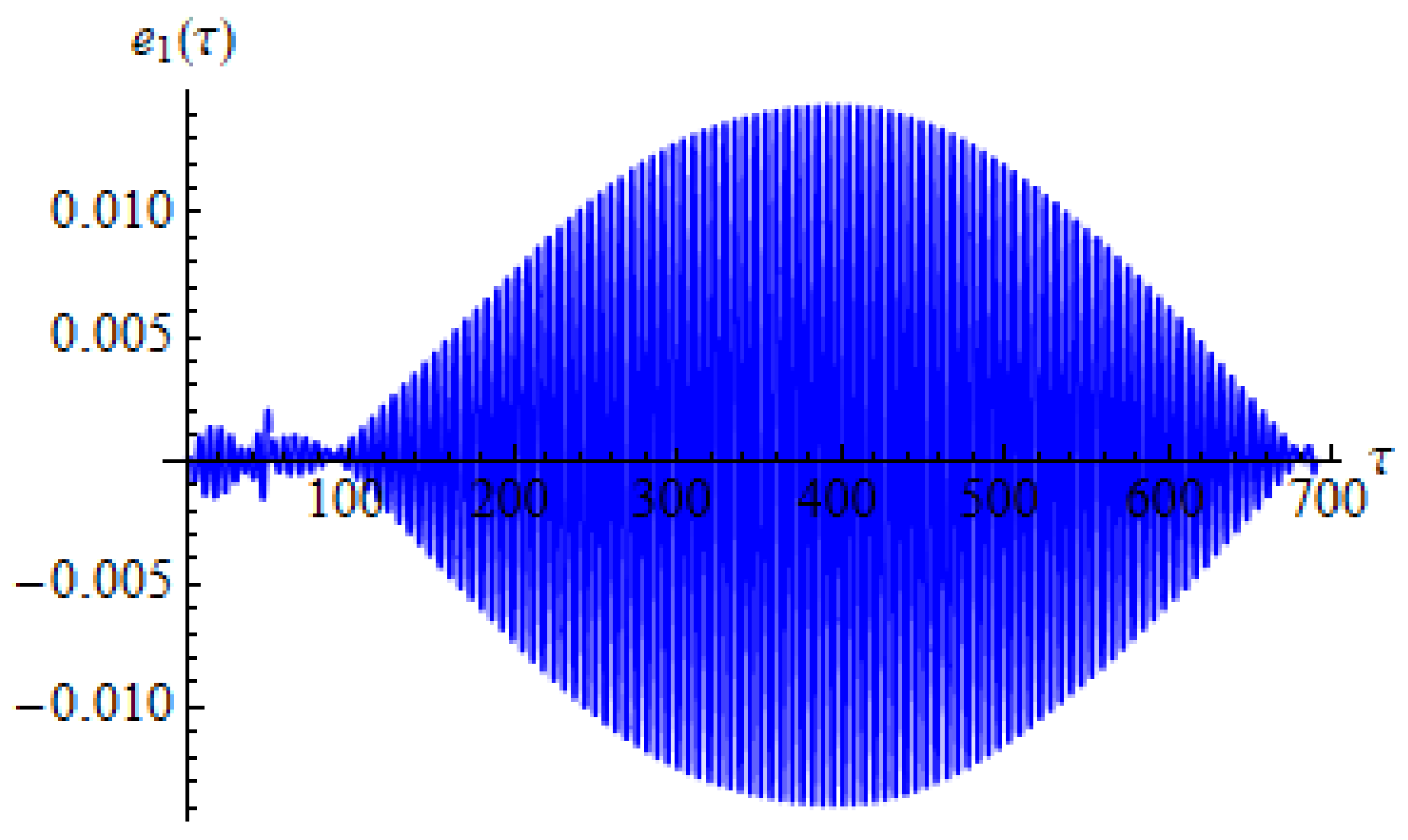
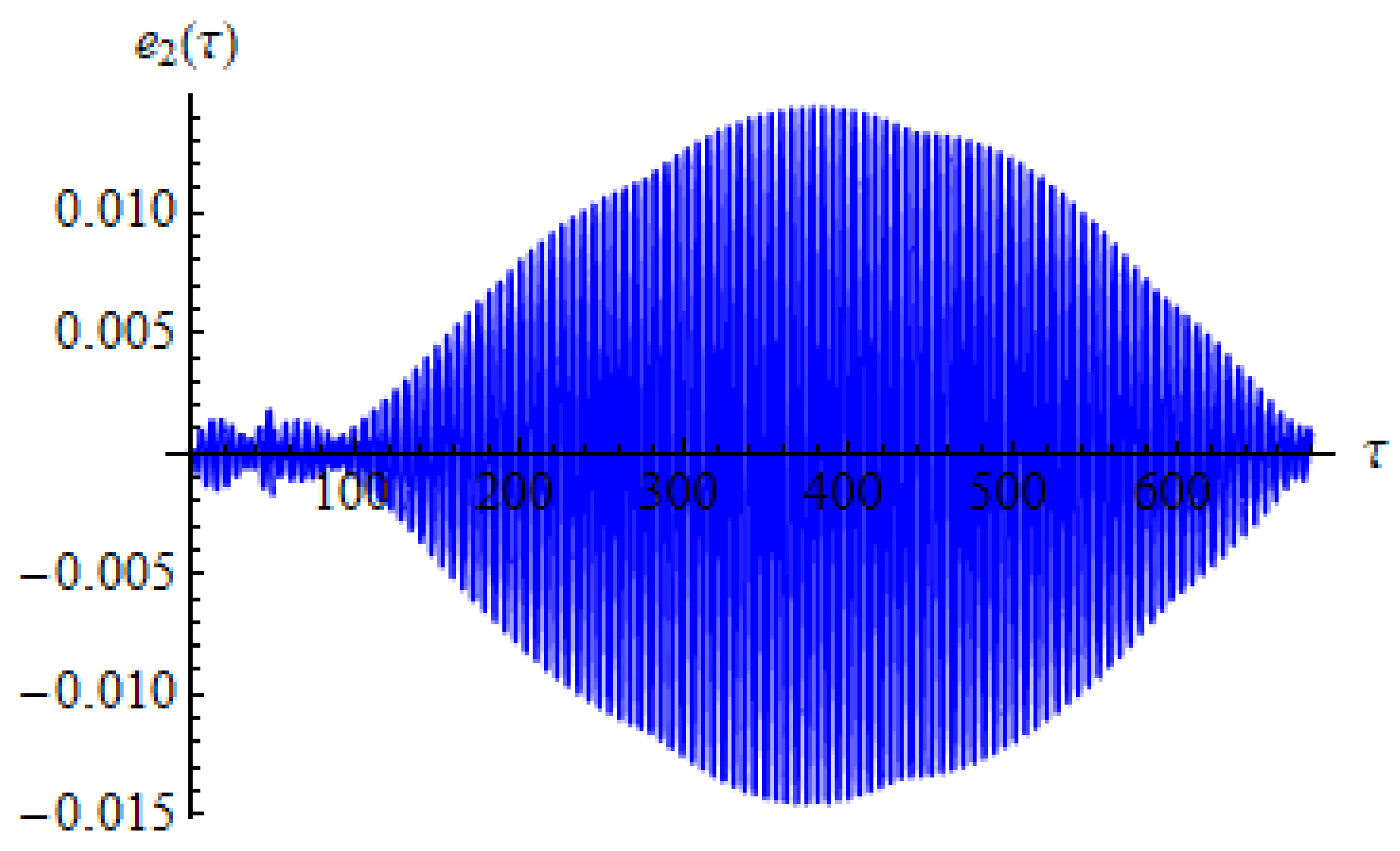
One defines the tracking errors e1 and e2 as
e 1 = x 1 x ˜ , e 2 = x 2 x ˜ + φ e 1
where x ˜ is the approximate analytical solution of Equations (7) and (10) above obtained by means of the OAFM, φ is a positive parameter and the control U will be defined later.
If μ ¯ , a ¯ 1 , a ¯ 2 , a ¯ 3 , a ¯ 4 , a ¯ 5 , Δ ¯ , β ¯ are defined as estimated parameters, then the estimation errors of parameters are defined as [25]:
μ ˜ = μ ¯ μ , a ˜ 1 = a ¯ 1 a 1 , a ˜ 2 = a ¯ 2 a 2 , a ˜ 3 = a ¯ 3 a 3 , a ˜ 4 = a ¯ 4 a 4 , a ˜ 5 = a ¯ 5 a 5 , Δ ˜ = Δ ¯ Δ , β ˜ = β ¯ β
The Lyapunov function is chosen in the form:
V ( e 1 , e 2 , μ ˜ , a ˜ i , Δ ˜ , β ˜ ) = 1 2 ( λ 1 e 1 2 + λ 2 e 2 2 + λ 3 μ ˜ 2 + λ 4 a ˜ 1 2 + λ 5 a ˜ 2 2 + λ 6 a ˜ 3 2 + λ 7 a ˜ 4 2 + λ 8 a ˜ 5 2 + λ 9 Δ ˜ 2 + λ 10 β ˜ 2 + λ 11 λ ˜ 2 )
where λj, j = 1, 2, …, 11 are positive parameters. The time derivative of Lyapunov function can be written, taking into consideration Equations (74), (75) and (76) in the form
d V d τ = λ 1 e 1 ( e 2 φ e 1 ) + λ 2 e 2 [ μ x 2 a 1 x 1 + γ a 2 x 1 2 a 3 x 1 3 a 4 x 1 4 a 5 x 1 5 + Δ cos ω τ + ( β sin Ω τ γ cos 2 Ω τ ) 1 + 4 x 1 3 R + 4 x 1 2 3 R 2 + 32 x 1 3 27 R 3 + 80 x 1 4 81 R 4 + 64 x 1 5 81 R 5 x ˜ + φ ( e 2 φ e 1 ) ] + λ 3 μ ˜ μ ˜ + λ 4 a ˜ 1 a ˜ 1 + λ 5 a ˜ 2 a ˜ 2 + + λ 6 a ˜ 3 a ˜ 3 + λ 7 a ˜ 4 a ˜ 4 + λ 8 a ˜ 5 a ˜ 5 + λ 9 Δ ˜ Δ ˜ + λ 10 β ˜ β ˜ + λ 11 γ ˜ γ ˜ )
We define the input control U through Equation (77) as:
U = μ ¯ x 2 + a ¯ 1 x 1 + a ¯ 2 x 1 2 + a ¯ 3 x 1 3 + a ¯ 4 x 1 4 + a ¯ 5 x 1 5 Δ cos ω τ ( β ¯ sin Ω τ γ ¯ cos 2 Ω τ ) 1 + 4 x 1 3 R + 4 x 1 2 3 R 2 + 32 x 1 3 27 R 3 + 80 x 1 4 81 R 4 + 64 x 1 5 81 R 5 + x ¯ φ e 2 γ ¯
Then Equation (77) can be rewritten through Equation (75) in the form:
d V d τ = λ 1 e 1 e 2 λ 1 φ e 1 2 + λ 2 [ μ ˜ x 2 + a ˜ 1 x 1 γ ˜ + a ˜ 2 x 1 2 + a ˜ 3 x 1 3 + a ˜ 4 x 1 4 + a ˜ 5 x 1 5 Δ ˜ cos ω τ ( β ˜ sin Ω τ γ ˜ cos 2 Ω τ ) 1 + 4 x 1 3 R + 4 x 1 2 3 R 2 + 32 x 1 3 27 R 3 + 80 x 1 4 81 R 4 + 64 x 1 5 81 R 5 e 2 λ 2 φ 2 e 1 e 2 + λ 3 μ ˜ μ ˜ + λ 4 a ˜ 1 a ˜ 1 + λ 5 a ˜ 2 a ˜ 2 + + λ 6 a ˜ 3 a ˜ 3 + λ 7 a ˜ 4 a ˜ 4 + λ 8 a ˜ 5 a ˜ 5 + λ 9 Δ ˜ Δ ˜ + λ 10 β ˜ β ˜ + λ 11 γ ˜ γ ˜
After some manipulations, Equation (79) becomes:
d V d τ = ( λ 1 φ 2 λ 2 ) e 1 e 2 λ 1 φ e 1 2 + μ ˜ ( λ 2 x 2 e 2 + λ 3 μ ˜ ) + a ˜ 1 ( λ 2 x 1 e 2 + λ 4 a ˜ ) + a ˜ 2 ( λ 2 x 1 2 e 2 + λ 5 a ˜ 2 ) + + a ˜ 3 ( λ 2 x 1 3 e 2 + λ 6 a ˜ 3 ) + a ˜ 4 ( λ 2 x 1 4 e 2 + λ 7 a ˜ 4 ) + a ˜ 5 ( λ 2 x 1 5 e 2 + λ 8 a ˜ 5 ) + Δ ˜ ( λ 9 Δ ˜ λ 2 e 2 cos ω τ ) + + β ˜ ( λ 10 β ˜ 1 + 4 x 1 3 R + 4 x 1 2 3 R 2 + 32 x 1 3 27 R 3 + 80 x 1 4 81 R 4 + 64 x 1 5 81 R 5 λ 2 e 2 sin Ω τ ] γ ˜ [ λ 2 e 2 1 + 4 x 1 3 R + + 4 x 1 2 3 R 2 + 32 x 1 3 27 R 3 + 80 x 1 4 81 R 4 + 64 x 1 5 81 R 5 λ 2 e 2 sin Ω τ γ ˜ [ λ 2 e 2 1 + 4 x 1 3 R + 4 x 1 2 3 R 2 + 32 x 1 3 27 R 3 + 80 x 1 4 81 R 4 + + 64 x 1 5 81 R 5 λ 2 e 2 cos 2 Ω τ λ 11 γ ˜ ]
The estimate parameters μ ˜ , a ˜ i , β ˜ , γ ˜ , i = 1, 2, …, 5 which appear in the last equation are defined as:
d μ ˜ d τ = λ 2 λ 3 x 2 e 2 ; d a ˜ 1 d τ = λ 2 λ 4 x 1 e 2 ; d a ˜ 2 d τ = λ 2 λ 5 x 1 2 e 2 ; d a ˜ 3 d τ = λ 2 λ 6 x 1 3 e 2 ; d a ˜ 4 d τ = λ 2 λ 7 x 1 4 e 2 d a ˜ 5 d τ = λ 2 λ 8 x 1 5 e 2 ; d Δ ˜ d τ = λ 2 λ 9 e 2 cos τ ; d β ˜ d τ = λ 2 λ 10 e 2 1 + 4 x 1 3 R + 4 x 1 2 3 R 2 + 32 x 1 3 27 R 3 + 80 x 1 4 81 R 4 + 64 x 1 5 81 R 5 sin Ω τ d γ ˜ d τ = λ 2 λ 11 e 2 1 1 + 4 x 1 3 R + 4 x 1 2 3 R 2 + 32 x 1 3 27 R 3 + 80 x 1 4 81 R 4 + 64 x 1 5 81 R 5 cos Ω τ
or taking into account Equations (73) and (74):
d μ ˜ d τ = λ 2 λ 3 x [ x x ˜ + φ ( x x ˜ ) ] ; d a ˜ 1 d τ = λ 2 λ 4 x [ x x ˜ + φ ( x x ˜ ) ] ; d a ˜ 2 d τ = λ 2 λ 5 x 2 [ x x ˜ + φ ( x x ˜ ) ] d a ˜ 3 d τ = λ 2 λ 6 x 3 [ x x ˜ + φ ( x x ˜ ) ] ; d a ˜ 4 d τ = λ 2 λ 7 x 4 [ x x ˜ + φ ( x x ˜ ) ] ; d a ˜ 5 d τ = λ 2 λ 8 x 5 [ x x ˜ + φ ( x x ˜ ) ] d Δ ˜ d τ = λ 2 λ 9 x 3 [ x x ˜ + φ ( x x ˜ ) ] cos Ω τ ; d β ˜ d τ = λ 2 λ 10 [ x x ˜ + φ ( x x ˜ ) ] 1 + 4 x 1 3 R + 4 x 1 2 3 R 2 + 32 x 1 3 27 R 3 + 80 x 1 4 81 R 4 + + 64 x 1 5 81 R 5 ; d γ ˜ d τ = λ 2 λ 11 [ x x ˜ + φ ( x x ˜ ) ] 1 1 + 4 x 1 3 R + 4 x 1 2 3 R 2 + 32 x 1 3 27 R 3 + 80 x 1 4 81 R 4 + 64 x 1 5 81 R 5 cos 2 Ω τ
In this way the Equation (80) becomes:
d V d τ = ( λ 1 φ 2 λ 2 ) e 1 e 2 λ 1 φ e 1 2
The positive parameter φ defined in Equation (74) is chosen as
φ = λ 1 λ 2 1
and therefore Equation (83) can be rewritten in the final form
d V d τ = λ 1 3 / 2 λ 2 1 / 2 e 1 2
It is clear that d V d τ < 0 .
Using the Lyapunov function and La Salle’s invariance principle, the system studied in the present work is globally asymptotically stable since the function V is a positive defined function and dV/dτ is negative definite.
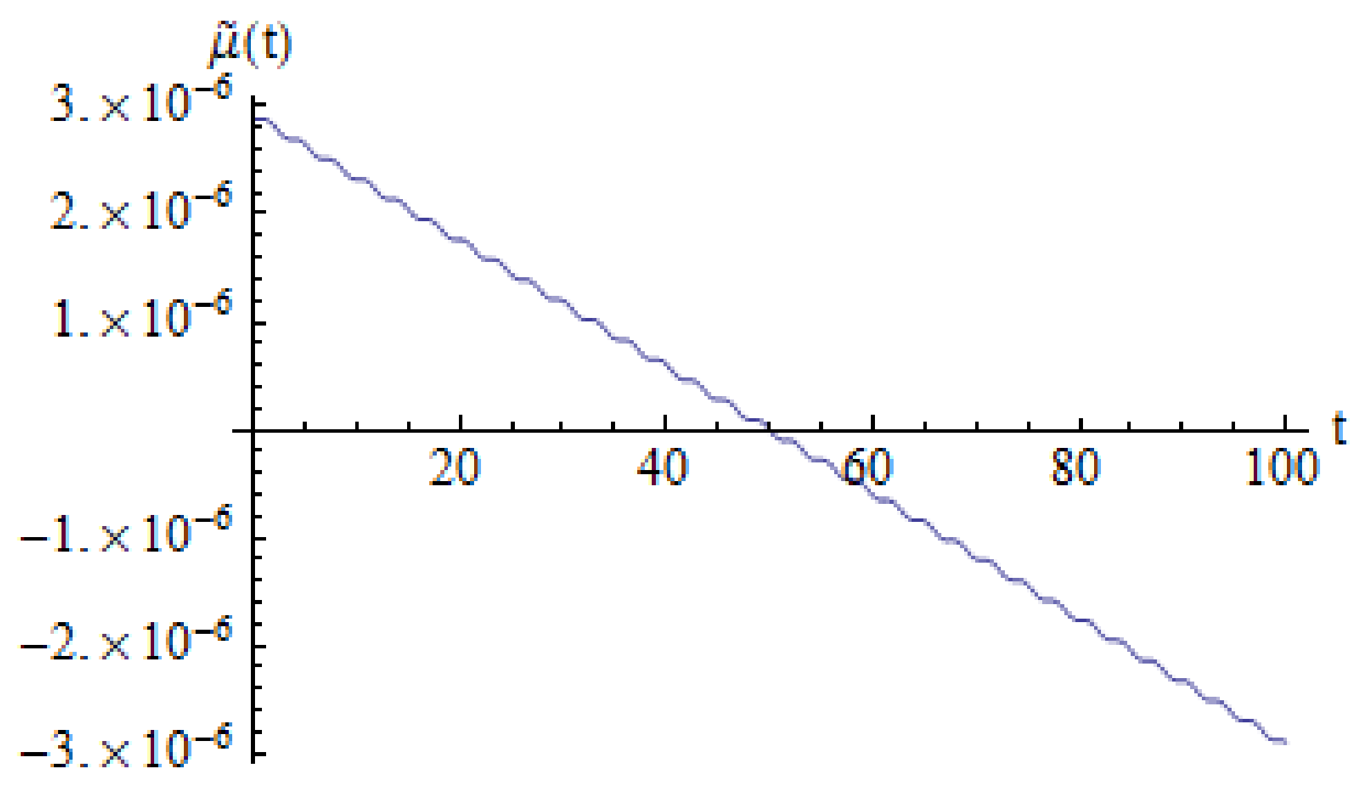
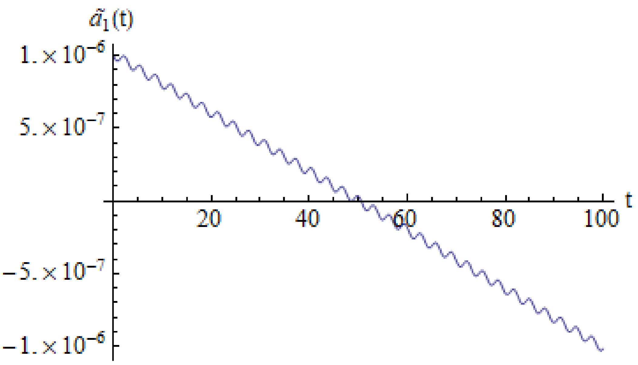
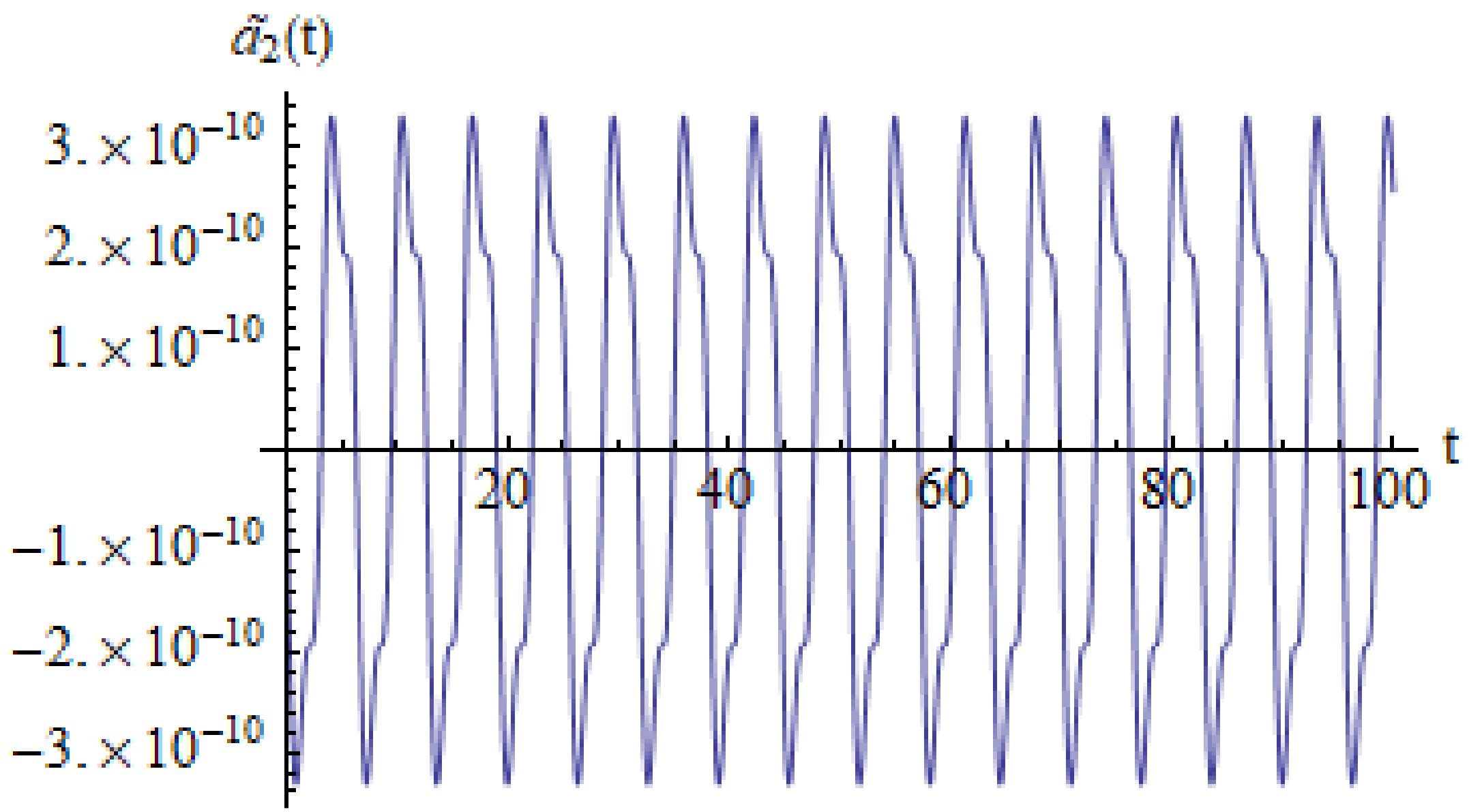
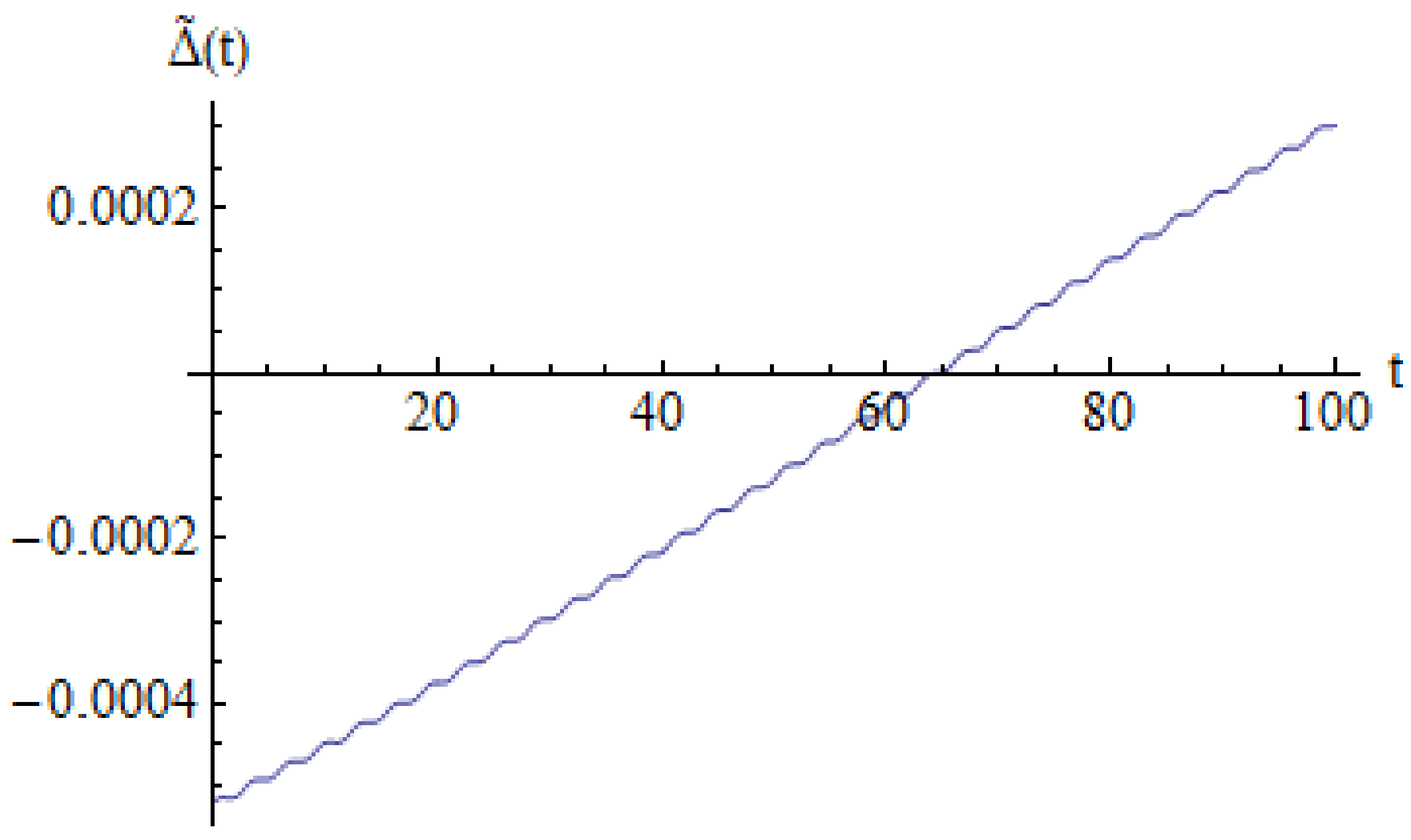
Figure 23 and Figure 24 depict the tracking errors e1 and e2, respectively.
In Figure 25, Figure 26, Figure 27 and Figure 28 are depicted only the variations of the parameters μ ˜ , a 1 ˜ , a 2 ˜ and Δ ˜ . In this way, it is clear that the Lyapunov function is well-defined.
The values of the errors e1 and e2 show that OAFM is a very efficient procedure and the estimate parameters show that the Lyapunov function can be practically determined, not only theoretically.

7. Conclusions

In the present work, the action of a vibro-impact nonlinear, damped, forced oscillator on the DC and AC electromagnetic actuation near the primary resonance is analyzed. The vibro-impact regime appears by the presence of Hertzian contact. This contact is supposed to be elastic and is maintained. The governing equation of motion is a nonlinear differential equation with variable coefficients. To find an approximate analytical solution of nonlinear differential equation we used a very accurate, effective and simple procedure, namely the Optimal Auxiliary Functions Method (OAFM). The governing equation is reduced to only two linear differential equations. The main novelties of our technique are the presence of so-called auxiliary functions, some convergence-control parameters, the construction of the two iterations, and the freedom to choose the procedure to determine the optimal values of the convergence-control parameters by applying rigorous mathematical procedures.
Also, we analyzed the local stability using some notions as the transformation averaging method, bookkeeping parameters, Jacobian matrix, or Routh-Hurwitz criteria. The borderline cases are presented for different values of the parameters. Global stability is studied by both Lyapunov function and La Salle’s invariance principle. These results lead to the conclusion that it is possible to control the nonlinear characteristics of the response near the primary resonance by tuning intensity of DC and AC electromagnetic actuation. Moreover, the proposed technique can be useful in certain engineering applications where the operating frequency range includes some critical frequencies that should be avoided.
Taking into account the proved performance of the OAFM technique, the proposed approach could be easily extended to other real practical applications from other fields of research, such as fluid dynamics, astronomy, mechanics, electrical machines, where nonlinear dynamical systems are involved.

Author Contributions

Conceptualization, V.M., N.H., L.C. and B.M.; methodology, V.M., B.M. and N.H.; software, N.H. and B.M.; validation, N.H., B.M. and V.M.; formal analysis, V.M. and L.C.; investigation, V.M., B.M., L.C. and N.H.; resources, N.H.; data curation, V.M., B.M. and N.H.; writing—original draft preparation, N.H. and V.M.; writing—review and editing, N.H. and V.M.; visualization, N.H.; supervision, N.H.; project administration, N.H. All authors have read and agreed to the published version of the manuscript.

Funding

This research received no external funding.

Data Availability Statement

Not applicable.

Conflicts of Interest

The authors declare no conflict of interest.

References

  1. Song, Y.; Wang, Z.; Liu, Z.; Wang, R. A spatial coupling model to study dynamic performance of pantograph-catenary with vehicle-track excitation. Mech. Syst. Signal Process. 2021, 151, 107336. [Google Scholar] [CrossRef]
  2. Flour, L. Contact fatigue of automotive gears: Evolution and effects of residual stresses introduced by surface treatments. Fatigue Fract. Eng. Mater. Struct. 2000, 23, 217–228. [Google Scholar]
  3. Gonzalez-Perez, I.; Iserte, J.L.; Fuentes, A. Implementation of Hertz theory and validation of a finite element model for stress analysis of gear drives with localized bearing contact. Mech. Mach. Theory 2011, 46, 765–783. [Google Scholar] [CrossRef]
  4. Bichri, A.; Belhaq, M.; Liaudet, J.P. Effect of electromagnetic actuation on contact loss in a Hertzian contact oscillator. J. Comput Nonlyn. Dyn. 2015, 10, 064501. [Google Scholar] [CrossRef]
  5. Mann, B.P.; Carter, R.E.; Hazra, S.S. Experimental study of an impact oscillator with viscoelastic and Hertzian contact. Nonlinear Dyn. 2007, 50, 587–596. [Google Scholar] [CrossRef]
  6. Ma, Q.L.; Kahraman, A.; Liaudet, J.P.; Rigaud, E. An investigation of steady-state dynamic response of a sphere-plane contact interface with contact loss. J. Appl. Mech. 2007, 74, 249–255. [Google Scholar] [CrossRef]
  7. Liaudet, J.P.; Sabot, J. Vibro-Impact Induced by Non-Linear Resonances in Hertzian Contacts. In Dynamics of Vibro-Impact Systems; Babitsky, V.I., Ed.; Springer: Berlin/Heidelberg, Germany, 1999; pp. 251–260. [Google Scholar]
  8. Popov, V.L. Rigorous Treatment of Contact Problem-Hertzian Contact. In Contact Mechanics and Friction; Section 5; Springer: Berlin/Heidelberg, Germany, 2010. [Google Scholar]
  9. Axinte, T. Hertz contact problem between wheel and rail. Adv. Mat. Res. 2013, 337, 733–738. [Google Scholar] [CrossRef]
  10. Liaudet, J.P.; Rigaud, E. Superharmonic resonance of order 2 for an impacting Hertzian contact oscillator: Theory and experiments. Trans. ASME 2007, 7, 190–196. [Google Scholar]
  11. Bichri, A.; Belhaq, M.; Liaudet, J.P. Control of vibroimpact dynamics of a single-sided Hertzian contact forced oscillator. Nonlinear Dyn. 2011, 63, 51–60. [Google Scholar] [CrossRef]
  12. Mokni, L.; Bichri, A.; Belhaq, M. Effect of time delay on vibroimpact dynamics in a forced Hertzian contact oscillator. MATEC Web Conf. 2012, 1, 02002. [Google Scholar] [CrossRef]
  13. Bichri, A.; Belhaq, M. Control of a forced impacting Hertzian contact oscillator near sub-and superharmonic resonance of order 2. J. Comput Nonlyn. Dyn. 2012, 7, 011003. [Google Scholar] [CrossRef]
  14. Kirrou, I.; Belhaq, M. Contact stiffness modulation on contact-mode atomic force microscopy. Int. J. Non-Linear Mech. 2013, 55, 102–109. [Google Scholar] [CrossRef]
  15. Belhaq, M.; Bichri, A.; Hagopian, J.; Mahfoud, J. Effect of electromagnetic actuation on the dynamics of a harmonically excited cantilever beam. Int. J. Non-Linear Mech. 2011, 46, 828–833. [Google Scholar] [CrossRef]
  16. Bichri, A.; Belhaq, M.; Mahfoud, J. Effect of a high-frequency AC electromagnetic actuation on the dynamic of an excited cantilever beam. MATEC Web Conf. 2014, 16, 08002. [Google Scholar] [CrossRef]
  17. Pereira, I.A.; Leao, L.S.; Carvalho, F.C.; Cavalini Junior, A.A.; Junior, V.S. Vibration suppression on a rotating machine by the use of electromagnetic actuators and a PID controller. In Proceedings of the XXVI Congresso Nacional de Estudiantes de Engenharia Mecanica, Ilhéus, Brasil, 19–23 August 2019. [Google Scholar]
  18. Zhang, J.; Yang, K.; Li, R. A bistable nonlinear electromagnetic actuator with elastic boundary for actuation performance improvement. Nonlinear Dyn. 2020, 100, 3575–3596. [Google Scholar] [CrossRef]
  19. Tang, M.; Boswald, M.; Govers, Y.; Pusch, M. Identification and assessment of a nonlinear dynamic actuated model for controlling an experimental flexible ring. CEAS Aeronaut. J. 2021, 12, 413–426. [Google Scholar] [CrossRef]
  20. Zhang, M.; Li, Q. A compound scheme based on improved ADRC and nonlinear compensation for electromechanical actuator. Actuators 2022, 11, 93. [Google Scholar] [CrossRef]
  21. Xiao, H.; Brennan, M.J.; Shao, Y. On the undamped free vibration of a mass interacting with a Hertzian contact stiffness. Mech. Res. Commun. 2011, 38, 560–564. [Google Scholar] [CrossRef]
  22. Ali, F. Numerical study on subsurface-stress in Hertzian contacts under pure sliding conditions. J. Appl. Comput. Mech. 2020, 6, 1098–1106. [Google Scholar]
  23. Quazi, A.; Sebes, M.; Chollet, H.; Yin, H.; Pozzolini, C. An extension of FASTSIM for state non-Hertzian contact. In Proceedings of the 27th IAVSD Symposium on Dynamics of Vehicles on Roads and Tracks, Saint Petersburg, Russia, 16–20 August 2011. [Google Scholar]
  24. Ciulli, E.; Betti, A.; Forte, P. The applicability of the Hertzian formulas to point contacts of spheres and spherical caps. Lubricants 2022, 10, 233. [Google Scholar] [CrossRef]
  25. Constandinou, S.; Blackford, J.R.; Haxley, K.J. Quantifying Errors Due to the Hertzian Contact Model in Multi-Sphere Discrete Element Modeling Simulations. Porceedings of the 8th European Congress on Computational Methods on Applied Sciences and Engineering, Oslo, Norway, 5–9 June 2022. [Google Scholar]
  26. Wu, C.E.; Lin, K.H.; Juang, J.Y. Hertzian load-displacement relation holds for spherical indentation on soft elastic solids undergoing large deformations. Tribol. Int. 2016, 97, 71–76. [Google Scholar] [CrossRef]
  27. Vouaillat, G.; Noyel, J.P.; Ville, F.; Kleber, X.; Rathery, S. From Hertzian contact to spur gears: Analyses of stresses and rolling contact fatigue. Mech. Ind. 2019, 20, 626. [Google Scholar] [CrossRef]
  28. Yousuf, L.S. Deflection calculation of cam profile due to a Hertzian contact pressure. J. Mech. 2020, 37, 149–160. [Google Scholar] [CrossRef]
  29. Cao, D.; Xia, W.; Hu, W. Low frequency and broadband vibration analysis energy harvester driven by mechanical impact based on layer-separated piezoelectric beam. Appl. Math Mech. Engl. Ed. 2019, 40, 1777–1790. [Google Scholar] [CrossRef]
  30. Zhang, L.; Tang, X.; Qin, Z.; Chu, F. Vibro-impact energy harvester for low frequency vibration enhanced by acoustic black hole. Appl. Phys. Lett. 2022, 121, 013902. [Google Scholar] [CrossRef]
  31. Marinca, V.; Herisanu, N. Construction of analytical solution to axisymmetric flow and heat transfer on a moving cylinder. Symmetry 2020, 12, 1335. [Google Scholar] [CrossRef]
  32. Marinca, V.; Herisanu, N. Optimal Auxiliary Functions method for a pendulum wrapping on two cylinders. Mathematics 2020, 8, 1364. [Google Scholar] [CrossRef]
  33. Herisanu, N.; Marinca, V. An efficient analytical approach to investigate the dynamics of misalignment multirotor system. Mathematics 2020, 8, 1083. [Google Scholar] [CrossRef]
  34. Marinca, B.; Marinca, V.; Bogdan, C. Dynamics of SEIR epidemic model by Optimal Auxiliary Functions Method. Chaos Solitons Fractals 2021, 14, 110949. [Google Scholar] [CrossRef]
  35. Herisanu, N.; Marinca, V. A solution procedure combining analytical and numerical approaches to investigate a two-degree of freedom vibro-impact oscillator. Mathematics 2021, 9, 1374. [Google Scholar] [CrossRef]
  36. Herisanu, N.; Marinca, V. An effective analytical approach to nonlinear vibration of elastically actuated microtubes. Meccanica 2021, 56, 813–823. [Google Scholar] [CrossRef]
  37. Blekhman, I.I. Vibrational Mechanics: Nonlinear Dynamic Effects, General Approach, Applications; World Scientific: Singapore, 2000. [Google Scholar]
Figure 1. Sketch of damped forced Hertzian oscillator with two symmetric EA.
Mathematics 11 02194 g001
Figure 2. Comparison between the functions F1 and G1 for R = 1.
Mathematics 11 02194 g002
Figure 3. Comparison between the functions F2 and G2 for R = 1.
Mathematics 11 02194 g003
Figure 4. Comparison between the functions F3 and G3 for R = 1.
Mathematics 11 02194 g004
Figure 5. Comparison between the approximate solution (30) and numerical integration results for τ = [0,50] _ _ _ _analytical results; ______ numerical results.
Mathematics 11 02194 g005
Figure 6. Comparison between the approximate solution (36) and numerical integration results for τ > 50: _ _ _ _ analytical results; ______ numerical results.
Mathematics 11 02194 g006
Figure 7. Comparison between the approximate solution (7) and numerical integration results: _ _ _ _analytical results; ______ numerical results.
Mathematics 11 02194 g007
Figure 8. Illustration of W from Equation (62) for a1 = 1; a2 = 1/6; a3 = −1/54; a4 = 1/432; a5 = 1/1296; γ = 0.0002.
Mathematics 11 02194 g008
Figure 9. Illustration of A from Equation (61) for a1 = 1; a2 = 1/6; a3 = −1/54; a4 = 1/432; a5 = 1/1296; γ = 0.0002.
Mathematics 11 02194 g009
Figure 10. Illustration of B from Equation (61) for a1 = 1; a2 = 1/6; a3 = −1/54; a4 = 1/432; a5 = 1/1296; γ = 0.0002.
Mathematics 11 02194 g010
Figure 11. Illustration of W from Equation (62) for a1 = 0.75; a2 = 1/6; a3 = −1/54; a4 = 1/432; a5 = 1/1296; γ = 0.0002.
Mathematics 11 02194 g011
Figure 12. Illustration of A from Equation (61) for a1 = 0.75; a2 = 1/6; a3 = −1/54; a4 = 1/432; a5 = 1/1296; γ = 0.0002.
Mathematics 11 02194 g012
Figure 13. Illustration of B from Equation (61) for a1 = 0.75; a2 = 1/6; a3 = −1/54; a4 = 1/432; a5 = 1/1296; γ = 0.0002.
Mathematics 11 02194 g013
Figure 14. Illustration of W from Equation (62) for a1 = 2; a2 = 1/6; a3 = −1/54; a4 = 1/432; a5 = 1/1296; γ = 0.0002.
Mathematics 11 02194 g014
Figure 15. Illustration of A from Equation (61) for a1 = 2; a2 = 1/6; a3 = −1/54; a4 = 1/432; a5 = 1/1296; γ = 0.0002.
Mathematics 11 02194 g015
Figure 16. Illustration of B from Equation (61) for a1 = 2; a2 = 1/6; a3 = −1/54; a4 = 1/432; a5 = 1/1296; γ = 0.0002.
Mathematics 11 02194 g016
Figure 17. Illustration of W from Equation (62) for a1 = 1; a2 = 1/6; a3 = −1/54; a4 = 1/432; a5 = 1/1296; γ = 0.0005.
Mathematics 11 02194 g017
Figure 18. Illustration of A from Equation (61) for a1 = 1; a2 = 1/6; a3 = −1/54; a4 = 1/432; a5 = 1/1296; γ = 0.0005.
Mathematics 11 02194 g018
Figure 19. Illustration of B from Equation (61) for a1 = 1; a2 = 1/6; a3 = −1/54; a4 = 1/432; a5 = 1/1296; γ = 0.0005.
Mathematics 11 02194 g019
Figure 20. Illustration of W from Equation (62) for a1 = 1; a2 = 1/6; a3 = −1/54; a4 = 1/432; a5 = 1/1296; γ = 0.0001.
Mathematics 11 02194 g020
Figure 21. Illustration of A from Equation (61) for a1 = 1; a2 = 1/6; a3 = −1/54; a4 = 1/432; a5 = 1/1296; γ = 0.0001.
Mathematics 11 02194 g021
Figure 22. Illustration of B from Equation (61) for a1 = 1; a2 = 1/6; a3 = −1/54; a4 = 1/432; a5 = 1/1296; γ = 0.0001.
Mathematics 11 02194 g022
Figure 23. Tracking error e1.
Mathematics 11 02194 g023
Figure 24. Tracking error e2.
Mathematics 11 02194 g024
Figure 25. Variation of parameter μ ˜ .
Mathematics 11 02194 g025
Figure 26. Variation of parameter a 1 ˜ .
Mathematics 11 02194 g026
Figure 27. Variation of parameter a 2 ˜ .
Mathematics 11 02194 g027
Figure 28. Variation of parameter Δ ˜ .
Mathematics 11 02194 g028
Disclaimer/Publisher’s Note: The statements, opinions and data contained in all publications are solely those of the individual author(s) and contributor(s) and not of MDPI and/or the editor(s). MDPI and/or the editor(s) disclaim responsibility for any injury to people or property resulting from any ideas, methods, instructions or products referred to in the content.

