Finite-Time Adaptive Fuzzy Control for Unmodeled Dynamical Systems with Actuator Faults

Abstract

This article concentrates upon the issue of finite-time tracking control for a category of nonlinear systems in pure-feedback form with actuator faults and unmodeled dynamics, where the loss of effectiveness and bias fault are considered. Meanwhile, the function approximation method utilizing fuzzy logic systems and dynamic surface control approach with first-order filter are implemented to model the unknown nonlinear terms induced from the proposed controller procedure and tackle the “explosion of complexity” issue of the classic backstepping method. The use of the maximal norm of the weight vector estimation method and adaptive approach reduces the computation load induced by fuzzy logic systems. Within the framework of backstepping control, a finite-time adaptive fuzzy fault-tolerant control protocol is derived to guarantee the boundedness of all signals and tracking error of the controlled system within a finite-time. Simulation studies are offered to show the validity of the derived theoretical results of the finite-time control protocol.

1. Introduction

The backstepping-based control has undergone considerable development in its application to various types of systems and some significant results have been established [1,2,3,4]. However, when the nonlinear systems contain unknown functions, the backstepping-based control schemes are not feasible. Unfortunately, the assumption that the nonlinear system under consideration is totally known is quite restrictive for a variety of engineering systems. To relax this assumption, the function approximation method with neural networks (NNs) or fuzzy logic systems (FLSs) has been broadly employed to deal with the model uncertainty functions due to their great approximation ability [5,6,7]. Fruitful adaptive backstepping NNs or adaptive backstepping FLSs control protocols have been proposed and have been widely applied to engineering systems, such as unmanned aerial vehicles, autonomous underwater vehicles, satellite clusters, sensor networks, and so on [8,9,10,11]. Note the fact that the applicability of traditional adaptive NNs/FLSs backstepping methods requires recursive differentiation on virtual control inputs at every step. This can induce an explosion of complexity issues, which may intensify the computational requirements or even reduce the control performance. The dynamic surface control approach is an effective way to resolve this drawback [12]. Recently, numerous studies have focused on leveraging the dynamic surface control approach to design adaptive controllers for nonlinear uncertain systems [13,14].

On the other hand, in real-world industrial systems, various types of faults may occur, such as process failures, actuator faults, sensor failures, and communication failures, which can adversely affect the performance of the controlled systems, and in severe cases, result in instability [6]. With the aim of guaranteeing safe and reliable operations, studying fault-tolerant schemes is crucial. Therefore, researchers have developed control schemes that can take into account the presence of actuator faults and adapt to them [6,15,16]. By using the adaptive approach and command filter method, a tracking control strategy is given for a kind of switched systems subject to unmeasurable states and actuator fault in [6]. Based on the reinforcement learning algorithm, a fault-tolerant adaptive tracking controller is derived for discrete-time multiagent systems in [15]. In [16], an adaptive distributed fault-tolerant controller is derived for nonlinear multiagent systems, where the hybrid faults are considered. The proposed adaptive adjustable parameter method can improve the accuracy of the fault information value estimation by utilizing the output signal, which has been widely used in the fault-tolerant control research field. Further, to handle the nonaffine nonlinear faults, in [17], a prescribed performance fault-tolerant control strategy is developed utilizing the excellent approximation capabilities of FLSs. It is should be noted that the fault-tolerant controllers mentioned earlier can only ensure the controlled systems are asymptotically stable.

The majority of the current research focuses on infinite-time tracking control, which involves ensuring that the states of controlled systems can reach a specified reference signal as the convergence time tends to infinity. In industrial applications, it is necessary for the system to reach the desired signal within a finite time to achieve ideal robustness and performance. Therefore, the finite-time approach was used to design the tracking control schemes to attain high-speed convergence [13,18,19,20]. In comparison with asymptotic control methods, the finite-time control approaches not only provide better disturbance-rejection ability, higher tracking precision, and faster convergence rate but also ensure that the control aim is achievable within finite-time, rendering them more significant [21]. Thus, extensive research has been conducted by scholars on finite-time control methods for complicated industrial systems, such as aircraft, nuclear power stations, and high-performance automobiles [3,22,23,24,25]. Nonetheless, there is little research focusing on the issue of unmodeled dynamics resides. The issue of unmodeled dynamics is present in virtually all real-world systems due to measurement noise, external disturbances, and modeling inaccuracies. The presence of these factors often leads to the degradation of system performance and instability. Therefore, investigating the issue of unmodeled dynamics is highly critical, and numerous significant works have been given in [26,27,28]. Despite the considerable works reported, there is still an essential issue that requires to be tackled in finite-time tracking control for nonlinear systems with actuator faults and unknown functions, which will make the proposed control more challenging and complicated. Furthermore, when the unmodeled dynamics are incorporated, the control design becomes more difficult.

Motivated by the statements mentioned above, this article addresses the fault-tolerant finite-time issue for unmodeled dynamical systems with unknown functions. The superiority of the results shown in this article are given as follows: (1) As compared with recent results [6,15,16] on fault-tolerant control, which only emphasizes that the controlled systems are asymptotically stable, in this article, a new finite-time control scheme is derived for unmodeled dynamical nonlinear systems to guarantee finite-time tracking with bounded tracking error. (2) Different from the finite-time controllers in [29,30], the impact of the unmodeled dynamical and actuator faults is considered in this paper. By utilizing the FLSs and adaptive approach, the challenge regarding the presence of unmodeled dynamical and actuator faults is resolved, thus the control performance is not affected by the unmodeled dynamical and the fault-tolerant property is guaranteed. (3) To prevent the issue of “explosion of complexity” that is often associated with traditional backstepping methods, the controller design utilizes dynamic surface control technology featuring a first-order filter. In addition, by the maximal norm of the weight vector estimation method, only two adaptive parameters are required to derive the fuzzy control protocol for the unmodeled dynamical systems, which greatly reduce the computational load.

The rest of this article is outlined as follows. The problem statement and preliminaries are presented in Section 2. In Section 3, the adaptive fault-tolerant finite-time fuzzy controller design and the stability analysis are shown. In Section 4, simulation examples are shown. In Section 5, concluding remarks are provided.

Notations: ${\mathbb{R}}^{m\times n}$ denotes the set of $m\times n$ real matrices. $C^p$ means a function with p continuous derivative. $\parallel ·\parallel$ denotes the Euclidean norm. ${\mathrm{sig}}^{\mathrm{a}}(·)=\mathrm{sign}(·){|·|}^{\mathrm{a}}$, where $\mathrm{sign}(·)$ refers to the sign function.

2. Problem Statement and Preliminaries

2.1. System Description

In this paper, we consider the following strict-feedback uncertain nonlinear systems

$$\left\{\begin{array}{c}\dot{z}=q(z,x)\hfill \\ {\dot{x}}_1=x_2+f_1\left(x_1\right)+{\Delta }_1(x,z,t),\hfill \\ {\dot{x}}_m=x_{m+1}+f_m\left(x_m\right)+{\Delta }_m(x,z,t),2\le m\le n-1\hfill \\ {\dot{x}}_n=f_n\left({\overline{x}}_n\right)+u+{\Delta }_n(x,z,t),\hfill \\ y=x_1\hfill \end{array}\right.$$

(1)

where $x={[x_1,\dots ,x_n]}^T\in {\mathbb{R}}^n$, $u\in \mathbb{R}$, $y\in \mathbb{R}$, are the plant state vector, control input, and output of the system, respectively. $x_m={[x_1,\dots ,x_m]}^T\in {\mathbb{R}}^m$, $z\in \mathbb{R}$ is the unmeasured state. $q(·)$ and $f_i(·)$ are unknown Lipschitz continuous functions. ${\Delta }_i(·)\in \mathbb{R},i=1,\dots ,n$ is the nonlinear dynamic disturbance which is unknown Lipschitz continuous function.

For practical engineering, the actuator faults are a common occurrence, which can be modeled as

$$u^f=\hslash \left(t\right)u\left(t\right)+u_r\left(t\right)$$

(2)

where $\hslash \left(t\right)$ is time-varying unknown efficiency factor, which satisfies $0<\underline{\hslash }\le \hslash \left(t\right)\le 1$ with $\underline{\hslash }$ is the lower bound of $\hslash \left(t\right)$. $u_r\left(t\right)$ is bias fault, which can be described as the bounded time-varying functions. $u_r\left(t\right)$ satisfies $|u_r\left(t\right)|\le u_r^{\max }$.

Control objective: Given the desired signal $y_d$ for systems (1) with unmodeled dynamical and actuator faults, derive a finite-time adaptive fuzzy fault-tolerant control protocol such that the tracking error $y-y_d$ converges to a small region within finite-time, and all the closed-loop signals are SGPFS.

Lemma 1

([31]). If ${ı}_1>0$, ${ı}_2>0$, and $𝚥>0$, we have

$$\begin{array}{c}{\left|x\right|}^{{ı}_1}{\left|z\right|}^{{ı}_2}\le \frac{{ı}_1𝚥}{{ı}_1+{ı}_2}{\left|x\right|}^{{ı}_1+{ı}_2}+\frac{{ı}_2{𝚥}^{-{ı}_1/{ı}_2}}{{ı}_1+{ı}_2}{\left|z\right|}^{{ı}_1+{ı}_2}\end{array}$$

(3)

Lemma 2

([32]). If ${\varrho }_0>0$, we have

$$\begin{array}{c}\hfill 0\le |{\varrho }_0|-{\varrho }_0\tanh \left(\frac{{\varrho }_0}{\iota }\right)\le 0.2785\iota \end{array}$$

(4)

where $\iota >0$ is a constant.

Lemma 3

([32]). If $x\in R$ and $\zeta \in R$, one has

$$\begin{array}{c}\hfill x\zeta \le \frac{l^{{\varrho }_1}}{{\varrho }_1}{\left|x\right|}^{{\varrho }_1}+\frac{l}{b{l}^{{\varrho }_2}}{\left|\zeta \right|}^{{\varrho }_2}\end{array}$$

(5)

where $l>0$, ${\varrho }_1>1$, ${\varrho }_2>1$, and $({\varrho }_1-1)({\varrho }_2-1)=1$.

Lemma 4

([33]). Consider the nonlinear system

$$\dot{x}=f(x,t),$$

(6)

assume that there exists a positive-definite Lyapunov function $V\left(x\right):D\to R$ with $b>0$, $0<\alpha <1$, and $\mu >0$, such that

$$\dot{V}\left(x\right)\le -bV{\left(x\right)}^{\alpha }+\mu$$

(7)

then the system (6) is semiglobal practical finite-time stability (SGPFS).

Assumption 1

([34]). The reference signal $y_d$ and its first derivative ${\dot{y}}_d$ are bounded.

Assumption 2.

The ${\Delta }_i$ is unknown Lipschitz continuous function. Based on [35], the dynamic uncertainty ${\Delta }_i$ in (1) satisfies

$$|{\Delta }_i(x,z,t)|\le {\varpi }_{i1}\left(\right|{\overline{x}}_i\left|\right)+{\varpi }_{i2}\left(\right|z\left|\right)$$

(8)

where ${\varpi }_{i1}(·)$, $i=1,\dots ,n$ are non-negative smooth unknown functions, and ${\varpi }_{i2}(·)$ are non-negative strictly increasing functions.

Definition 1

([35]). A $C^1$ function V is said to be an ISpS (input-to-state practically stable)-Lyapunov function for system $\dot{x}=f(x,u)$ if there exist functions ${\psi }_1$, ${\psi }_2$ of class $K_{\infty }$ such that

$${\psi }_1\left(\right|x\left|\right)\le V\left(x\right)\le {\psi }_2\left(\right|x\left|\right),$$

(9)

there exist two constants $c>0$, $d_0\ge 0$ and a class $K_{\infty }$-function Υ such that

$$\frac{\partial V_z}{\partial x}f(x,u)\le -c_{0}V\left(x\right)+\mathsf{{\rm Y}}\left(\right|u\left|\right)+d_0$$

(10)

where Equation (10) holds with $d_0=0$, the function V is referred to as an ISS (input-to-state stable)-Lyapunov function.

Assumption 3

([35]). The $\dot{z}=q(z,x)$ has an ISpS Lyapunov function $V_z\left(z\right)$ in the sense of Definition 1, there exists two constants $c>0$, $d_0\ge 0$ and three class $K_{\infty }$-functions ${\psi }_1$, ${\psi }_2$, and Υ such that a function $V_z\left(z\right)$ such that

$${\psi }_1\left(\right|z\left|\right)\le V_z\left(z\right)\le {\psi }_2\left(\right|z\left|\right),\frac{\partial V_z}{\partial z}\left(z\right)q(z,x)\le -c_0{V}_z\left(z\right)+\mathsf{{\rm Y}}\left(\right|x_1\left|\right)+d_0$$

(11)

moreover, $\overline{c}\in (0,c_0)$, $d_0$, Υ, ${\psi }_1$ are known.

The dynamical signal is constructed as follows

$$\dot{\kappa }=-\overline{c}\kappa +\overline{\mathsf{{\rm Y}}}\left(\right|x_1\left|\right)+d_0,\kappa \left(0\right)={\kappa }_0$$

(12)

where $\overline{\mathsf{{\rm Y}}}\left(\right|x_1\left|\right)\ge \mathsf{{\rm Y}}\left(\right|x_1\left|\right)$, $\overline{c}\in (0,c_0)$, and $c_0>0$ is a constant.

Lemma 5

([28]). According to (12) and Assumption 3, we have

$$V_z\left(z\right)\le \kappa \left(t\right)+B\left(t\right)$$

(13)

for all $t\ge 0$, where $B\left(t\right)$ is a non-negative function and $B\left(t\right)=0$ for $t\ge T_0$ with $T_0=T_0(\overline{c},{\kappa }_0,z_0)$ being finite time.

Moreover, we have

$$\dot{\kappa }=-\overline{c}\kappa +x_1^2\mathsf{{\rm Y}}\left(x_1^2\right)+d_0,\kappa \left(0\right)={\kappa }_0$$

(14)

where $\overline{\mathsf{{\rm Y}}}\left(\right|x_1\left|\right)=x_1^2\mathsf{{\rm Y}}\left(x_1^2\right)$.

2.2. Fuzzy-Logic Systems

The FLSs in this paper are designed using the following IF-THEN rules:

$$R^l:\mathrm{IF}{x}_1\mathrm{is}{F}_1^l,x_2\mathrm{is}{F}_2^l,\dots ,\mathrm{and}{x}_n\mathrm{is}{F}_n^l,\mathrm{THEN}y\mathrm{is}{G}^l,l=1,2,\dots ,g$$

(15)

where $x={[x_1,\dots ,x_n]}^T\in {\mathbb{R}}^n$ and $y\in \mathbb{R}$ refer to the FLSs input and output, respectively, $F_i^l$ and $G^l$ are the fuzzy sets associate with the membership functions ${\mu }_{F_i^l}\left(x_i\right)$ and ${\mu }_{G^l}\left(y\right)$, respectively. g is the number of rules.

Then, the FLSs can be modeled as

$$y\left(x\right)=\frac{{\sum }_{l=1}^g{\Lambda }_l{\prod }_{i=1}^n{\mu }_{F_i^l}\left(x_i\right)}{{\sum }_{l=1}^g{\prod }_{i=1}^n{\mu }_{F_i^l}\left(x_i\right)}$$

(16)

where ${\Lambda }_l={\max }_{y\in \mathbb{R}}{\mu }_{G^l}\left(y\right)$, and the fuzzy basis functions can be modeled by

$${\phi }_l\left(x\right)=\frac{{\prod }_{i=1}^n{\mu }_{F_i^l}\left(x_i\right)}{{\sum }_{l=1}^g[{\prod }_{i=1}^n{\mu }_{F_i^l}\left(x_i\right)]}$$

(17)

Denote ${\theta }^T=[{\Lambda }_1,{\Lambda }_2,\dots ,{\Lambda }_g]=[{\theta }_1,{\theta }_2,\dots ,{\theta }_g]$ and ${\phi }^T\left(x\right)=[{\phi }_1\left(x\right),{\phi }_2\left(x\right),\dots ,{\phi }_g\left(x\right)]$. Then, we have

$$y\left(x\right)={\theta }^T\phi \left(x\right)$$

(18)

Lemma 6

([36]). Assuming $f\left(x\right)$ is a continuous function defined on a compact set $\mathfrak{A}$, then for any given positive constant $\epsilon >0$, it is possible to construct FLSs that satisfy the following inequality:

$$\underset{\mathrm{x}\in \mathfrak{A}}{\sup }|f\left(x\right)-{\theta }^{\ast T}\phi \left(x\right)|\le \epsilon$$

(19)

3. Main Results

In this section, a finite-time adaptive fuzzy fault-tolerant control protocol for unmodeled dynamical nonlinear systems will be proposed by utilizing the dynamic surface technique with first-order filter and backstepping method.

3.1. Finite-Time Adaptive Fuzzy Fault-Tolerant Control Protocol

Prior to designing the controller, a sequence of function transformations is described through the following steps

$$\begin{array}{cc}\hfill e_1& =x_1-y_d\hfill \\ \hfill e_i& =x_i-{\alpha }_{i,L}i=2,3,\dots ,n\hfill \\ \hfill {\eta }_i& ={\alpha }_{i,L}-{\alpha }_{i-1}\hfill \end{array}$$

(20)

where ${\alpha }_{i-1}$ is the virtual control. ${\alpha }_{i,L}$ denotes the output of the first-order filter, which is defined as

$$\begin{array}{c}\hfill {\sigma }_i{\dot{\alpha }}_{i,L}+{\alpha }_{i,L}={\alpha }_{i-1},{\alpha }_{i,L}\left(0\right)={\alpha }_{i-1}\left(0\right),i=2,3,\dots ,n\end{array}$$

(21)

where ${\sigma }_i$ is a positive constant.

Remark 1.

The backstepping technique, which involves repeated differentiation of the virtual control signal ${\alpha }_{i-1}$, is widely recognized as a potential cause of the “explosion of complexity”. To address the “explosion of complexity” issue, the approach adopted is the utilization of the dynamic surface control technique, which incorporates a first-order filter (21). This filter is applied to ${\alpha }_{i-1}$ to produce the filtered signal ${\alpha }_{i,L}$, which is free from the explosion of complexity. This filtered signal is then utilized to the design of the control scheme. As a result, the occurrence of repeated differentiation can be efficiently avoided. The new function transformation $e_i=x_i-{\alpha }_{i,L}$ is defined by using the first-order filter to derive the finite-time tracking control protocol.

Remark 2.

This article adopts a first-order low-filter to avoid the algebraic error. However, this approach can cause a filtering error. This study is conducted without taking unexpected filtering errors into consideration. This undesirable error may degrade the control performance. According to [37], approaches to control based on a filtering-error compensation mechanism need to be explored in future.

Step 1: The time derivative of ${\dot{e}}_1$ yields

$$\begin{array}{cc}\hfill {\dot{e}}_1=& x_2+f_1\left(x_1\right)+{\Delta }_1(z,x,t)-{\dot{y}}_d\hfill \\ \hfill =& e_2+{\eta }_2+{\alpha }_1+f_1\left(x_1\right)+{\Delta }_1(z,x,t)-{\dot{y}}_d\hfill \end{array}$$

(22)

Define the Lyapunov function candidate as

$$V_1=\frac{1}{2}{e}_1^2+\frac{1}{2{\lambda }_{11}}{\tilde{\overline{\theta }}}_1^2+\frac{1}{2}{\eta }_2^2+\frac{1}{2{\lambda }_{12}}{\tilde{\overline{\varsigma }}}_1^2$$

(23)

Then, its time derivative is

$${\dot{V}}_1=e_1{\dot{e}}_1+\frac{1}{{\lambda }_{11}}{\tilde{\overline{\theta }}}_1{\dot{\tilde{\overline{\theta }}}}_1+\frac{1}{{\lambda }_{12}}{\tilde{\overline{\varsigma }}}_1{\dot{\tilde{\overline{\varsigma }}}}_1+{\eta }_2{\dot{\eta }}_2$$

(24)

Invoking (22), $e_1{\dot{e}}_1$ is calculated as

$$e_1{\dot{e}}_1=e_1(e_2+{\eta }_2+{\alpha }_1+f_1\left(x_1\right)+{\Delta }_1(z,x,t)-{\dot{y}}_d)$$

(25)

Then, we have

$${\dot{V}}_1=e_1(e_2+{\eta }_2+{\alpha }_1+f_1\left(x_1\right)+{\Delta }_1(z,x,t)-{\dot{y}}_d)+\frac{1}{{\lambda }_{11}}{\tilde{\overline{\theta }}}_1{\dot{\tilde{\overline{\theta }}}}_1+\frac{1}{{\lambda }_{12}}{\tilde{\overline{\varsigma }}}_1{\dot{\tilde{\overline{\varsigma }}}}_1+{\eta }_2{\dot{\eta }}_2$$

(26)

In light of Young’s inequality, we have

$$e_1{\eta }_2\le \frac{1}{2}{e}_1^2+\frac{1}{2}{\eta }_2^2$$

(27)

Based on Assumption 2, the term $e_1{\Delta }_{i,1}(z,x,t)$ satisfies

$$e_1{\Delta }_1(z,x,t)\le |e_1|{\varpi }_{11}\left(\right|x_1\left|\right)+|e_1|{\varpi }_{12}\left(\right|z\left|\right)$$

(28)

According to Lemma 2, we have

$$|e_1|{\varpi }_{11}\left(\right|x_1\left|\right)\le e_1{\widehat{\varpi }}_{11}(x_1,e_1)+{\acute{\tau }}_{11}$$

(29)

where the terms ${\widehat{\varpi }}_{11}(x_1,e_1)$ and ${\acute{\tau }}_{11}$ is defined as

$${\widehat{\varpi }}_{11}(x_1,e_1)={\varpi }_{11}\left(\right|x_1\left|\right)\tanh \left(\frac{e_1{\varpi }_{11}\left(\right|x_1\left|\right)}{{\tau }_{11}}\right),{\acute{\tau }}_{11}=0.2785{\tau }_{11}>0$$

(30)

For the term $|e_1|{\varpi }_{12}\left(\right|z\left|\right)$, we have

$$\begin{array}{cc}\hfill |e_1|{\varpi }_{12}\left(\right|z\left|\right)\le & |e_1|{\varpi }_{12}\left({\psi }_1^{-1}(\kappa +B)\right)\hfill \\ \hfill \le & |e_1|{\varpi }_{12}\left({\psi }_1^{-1}\left(2\kappa \right)\right)+\left|e_1\right|{\varpi }_{12}\left({\psi }_1^{-1}\left(2B\right)\right)\hfill \\ \hfill \le & e_1{\widehat{\varpi }}_{12}(e_1,\kappa )+{\acute{\tau }}_{12}+\frac{1}{4}{e}_1^2+d_1\left(t\right)\hfill \end{array}$$

(31)

with

$$\begin{array}{c}\hfill {\acute{\tau }}_{12}=0.2785{\tau }_{12}>0,d_1\left(t\right)={\left({\varpi }_{12}\left({\psi }_1^{-1}\left(2B\right)\right)\right)}^2\\ \hfill {\widehat{\varpi }}_{12}(e_1,\kappa )={\varpi }_{12}\left({\psi }_1^{-1}\left(2\kappa \right)\right)\tanh \left(\frac{e_1{\varpi }_{12}\left({\psi }_1^{-1}\left(2\kappa \right)\right)}{{\tau }_{12}}\right)\end{array}$$

(32)

Substituting (27)–(31) into (26), we have

$$\begin{array}{cc}\hfill {\dot{V}}_1\le & \frac{1}{2}{e}_1^2+e_1{e}_2+\frac{1}{2}{\eta }_2^2+e_1({\alpha }_1+f_1\left(x_1\right)-{\dot{y}}_d)++\frac{1}{{\lambda }_{11}}{\tilde{\overline{\theta }}}_1{\dot{\tilde{\overline{\theta }}}}_1+\frac{1}{{\lambda }_{12}}{\tilde{\overline{\varsigma }}}_1{\dot{\tilde{\overline{\varsigma }}}}_1+{\eta }_2{\dot{\eta }}_2\hfill \\ & +e_1{\widehat{\varpi }}_{11}(x_1,e_1)+{\acute{\tau }}_{11}+e_1{\widehat{\varpi }}_{12}(e_1,\kappa )+{\acute{\tau }}_{12}+\frac{1}{4}{e}_1^2+d_1\left(t\right)\hfill \\ \hfill \le & e_1{e}_2+\frac{1}{2}{\eta }_2^2+e_1({\alpha }_1+{\chi }_1\left(X_1\right)-{\dot{y}}_d)+\frac{1}{{\lambda }_{11}}{\tilde{\overline{\theta }}}_1{\dot{\tilde{\overline{\theta }}}}_1+\frac{1}{{\lambda }_{12}}{\tilde{\overline{\varsigma }}}_1{\dot{\tilde{\overline{\varsigma }}}}_1+{\eta }_2{\dot{\eta }}_2\hfill \\ & +{\acute{\tau }}_{11}+{\acute{\tau }}_{12}+\frac{3}{4}{e}_1^2+d_1\left(t\right)\hfill \end{array}$$

(33)

where ${\chi }_1\left(X_1\right)={\widehat{\varpi }}_{11}(x_1,e_1)+{\widehat{\varpi }}_{12}(e_1,\kappa )+f_1\left(x_1\right),X_1={[x_1,e_1,\kappa ]}^T$.

Based on Lemma 6, the FLSs are applied to approximate ${\chi }_1\left(X_1\right)$ as follows

$${\chi }_1\left(X_1\right)={\phi }_1^T\left(X_1\right){\theta }_1^{\ast }+{\epsilon }_1$$

(34)

As ${\epsilon }_1$ is bounded, there exists a constant ${\overline{\varsigma }}_1$ that is positive, such that

$$|{\epsilon }_1|\le {\overline{\varsigma }}_1$$

(35)

Then, we have

$$\begin{array}{cc}\hfill {\dot{V}}_1\le & e_1{e}_2+\frac{1}{2}{\eta }_2^2+e_1({\alpha }_1+{\phi }_1^T\left(X_1\right){\theta }_1^{\ast }+{\epsilon }_1-{\dot{y}}_d)+\frac{1}{{\lambda }_{11}}{\tilde{\overline{\theta }}}_1{\dot{\tilde{\overline{\theta }}}}_1+\frac{1}{{\lambda }_{12}}{\tilde{\overline{\varsigma }}}_1{\dot{\tilde{\overline{\varsigma }}}}_1+{\eta }_2{\dot{\eta }}_2\hfill \\ & +{\acute{\tau }}_{11}+{\acute{\tau }}_{12}+\frac{3}{4}{e}_1^2+d_1\left(t\right)\hfill \end{array}$$

(36)

Then, the virtual controller ${\alpha }_1$ is defined as

$${\alpha }_1=-\frac{e_1{\widehat{\overline{\theta }}}_1^2}{\parallel e_1{\phi }_1^T\left(x_1\right)\parallel {\widehat{\overline{\theta }}}_1+{ϵ}_{11}^{\ast }}-\frac{e_1{\widehat{\overline{\varsigma }}}_1^2}{|e_1|{\widehat{\overline{\varsigma }}}_1+{ϵ}_{12}^{\ast }}+{\dot{y}}_d-\frac{1}{2}{\mathrm{sgn}}^{\beta }\left(e_1\right)-\frac{3}{4}{e}_1$$

(37)

$${\dot{\widehat{\overline{\theta }}}}_1=-{\lambda }_{11}{\widehat{\overline{\theta }}}_1+{\lambda }_{11}\parallel e_1{\phi }_1^T\left(x_1\right)\parallel$$

(38)

$${\dot{\widehat{\overline{\varsigma }}}}_1=-{\lambda }_{12}{\widehat{\overline{\varsigma }}}_1+{\lambda }_{12}\left|e_1\right|$$

(39)

where ${\mathrm{sgn}}^{\beta }\left(z_1\right)=\mathrm{sign}\left(z_1\right){\left|z_1\right|}^{\beta }$, $0<\beta <1$ is a positive design parameter, $\parallel {\theta }_1^{\ast }\parallel \le {\overline{\theta }}_1$, ${ϵ}_{11}^{\ast }=ϵ\ast \mathrm{sign}\left(\right|z_1|\parallel {\phi }_1^T\left(x_1\right)\parallel {\widehat{\overline{\theta }}}_1)$, ${ϵ}_{12}^{\ast }=ϵ\ast \mathrm{sign}\left(\right|z_1|{\widehat{\overline{\varsigma }}}_1)$, $ϵ>0$ is a positive constant.

Substituting (37)–(39) into (36), we have

$$\begin{array}{cc}\hfill {\dot{V}}_1\le & e_1{e}_2+\frac{1}{2}{\eta }_2^2+e_1(-\frac{e_1{\widehat{\overline{\theta }}}_1^2}{\parallel e_1{\phi }_1^T\left(x_1\right)\parallel {\widehat{\overline{\theta }}}_1+{ϵ}_{11}^{\ast }}-\frac{e_1{\widehat{\overline{\varsigma }}}_1^2}{|e_1|{\widehat{\overline{\varsigma }}}_1+{ϵ}_{12}^{\ast }}+{\dot{y}}_d-\frac{1}{2}{\mathrm{sgn}}^{\beta }\left(e_1\right)-\frac{3}{4}{e}_1\hfill \\ & +{\phi }_1^T\left(X_1\right){\theta }_1^{\ast }+{\epsilon }_1-{\dot{y}}_d)+\frac{1}{{\lambda }_{11}}{\tilde{\overline{\theta }}}_1{\dot{\tilde{\overline{\theta }}}}_1+\frac{1}{{\lambda }_{12}}{\tilde{\overline{\varsigma }}}_1{\dot{\tilde{\overline{\varsigma }}}}_1+{\eta }_2{\dot{\eta }}_2+{\acute{\tau }}_{11}+{\acute{\tau }}_{12}+\frac{3}{4}{e}_1^2+d_1\left(t\right)\hfill \\ \hfill \le & e_1{e}_2+\frac{1}{2}{\eta }_2^2-\frac{e_1^2{\widehat{\overline{\theta }}}_1^2}{\parallel e_1{\phi }_1^T\left(x_1\right)\parallel {\widehat{\overline{\theta }}}_1+{ϵ}_{11}^{\ast }}-\frac{e_1^2{\widehat{\overline{\varsigma }}}_1^2}{|e_1|{\widehat{\overline{\varsigma }}}_1+{ϵ}_{12}^{\ast }}-\frac{1}{2}{\mathrm{sgn}}^{\beta +1}\left(e_1\right)+\parallel e_1{\phi }_1^T\left(X_1\right)\parallel {\overline{\theta }}_1\hfill \\ & +{\tilde{\overline{\theta }}}_1({\widehat{\overline{\theta }}}_1-\parallel e_1{\phi }_1^T\left(x_1\right)\parallel )+{\tilde{\overline{\varsigma }}}_1({\widehat{\overline{\varsigma }}}_1-|e_1\left|\right)+{\eta }_2{\dot{\eta }}_2+{\acute{\tau }}_{12}+{\acute{\tau }}_{11}+d_1\left(t\right)+|e_1\left|\right|{\epsilon }_1|\hfill \end{array}$$

(40)

Applying the fact that ${\phi }_1^T(·){\phi }_1(·)\le 1$, we have

$$\parallel e_1{\phi }_1^T\left(x_1\right)\parallel {\overline{\theta }}_1-\frac{e_1^2{\widehat{\overline{\theta }}}_1^2}{\parallel e_1{\phi }_1^T\left(x_1\right)\parallel {\widehat{\overline{\theta }}}_1+{ϵ}_{11}^{\ast }}-{\tilde{\overline{\theta }}}_1\parallel e_1{\phi }_1^T\left(x_1\right)\parallel =\frac{\parallel e_1{\phi }_1^T\parallel {\widehat{\overline{\theta }}}_1{ϵ}_{11}^{\ast }}{\parallel e_1{\phi }_1^T\left(x_1\right)\parallel {\widehat{\overline{\theta }}}_1+{ϵ}_{11}^{\ast }}\le ϵ$$

(41)

Similar to (41), one has

$$|e_1\left|\right|{\epsilon }_1|-\frac{e_1^2{\widehat{\overline{\varsigma }}}_1^2}{|e_1|{\widehat{\overline{\varsigma }}}_1+{ϵ}_{12}^{\ast }}-{\tilde{\overline{\varsigma }}}_1\left|e_1\right|\le \frac{e_1{\widehat{\overline{\varsigma }}}_1{ϵ}_{12}^{\ast }}{|e_1|{\widehat{\overline{\varsigma }}}_1+{ϵ}_{12}^{\ast }}\le ϵ$$

(42)

From (41) and (42), we have

$$\begin{array}{cc}\hfill {\dot{V}}_1\le & e_1{e}_2+\frac{1}{2}{\eta }_2^2-\frac{1}{2}{\mathrm{sgn}}^{\beta +1}\left(e_1\right)+{\tilde{\overline{\theta }}}_1{\widehat{\overline{\theta }}}_1+{\tilde{\overline{\varsigma }}}_1{\widehat{\overline{\varsigma }}}_1+{\eta }_2{\dot{\eta }}_2+{\acute{\tau }}_{11}+{\acute{\tau }}_{12}+d_1\left(t\right)+2ϵ\hfill \end{array}$$

(43)

Since ${\dot{\eta }}_2={\dot{\xi }}_2+s_2$ where ${\dot{\xi }}_2=-\frac{{\eta }_2}{{\sigma }_2}$, $s_2=-{\dot{\alpha }}_1$. From [38], we know ${\eta }_2$ is a continuous function. Based on Lemma 3, one obtains

$${\eta }_2{\dot{\eta }}_2=-\frac{{\eta }_2^2}{{\sigma }_2}+s_2{\eta }_2\le (\frac{1}{4{\ell }^2}-\frac{1}{{\sigma }_2}){\eta }_2^2+{\ell }^2{s}_2^2$$

(44)

where ℓ is a nonzero constant.

Furthermore, one has

$$\frac{1}{2}{\eta }_2^2+{\eta }_2{\dot{\eta }}_2=-(\frac{1}{{\sigma }_2}-\frac{1}{4{\ell }^2}-\frac{1}{2}){\eta }_2^2+{\ell }^2{s}_2^2$$

(45)

where ${\sigma }_2$ and ℓ are positive constants satisfying $\frac{1}{{\sigma }_2}-\frac{1}{4{\ell }^2}-\frac{1}{2}>0$.

Invoking (45) and (44), one has

$$\begin{array}{cc}\hfill {\dot{V}}_1\le & e_1{e}_2-\frac{1}{2}{\mathrm{sgn}}^{\beta +1}\left(e_1\right)+{\tilde{\overline{\theta }}}_1{\widehat{\overline{\theta }}}_1+{\tilde{\overline{\varsigma }}}_1{\widehat{\overline{\varsigma }}}_1+{\acute{\tau }}_{11}+{\acute{\tau }}_{12}+d_1\left(t\right)+2ϵ\hfill \\ & -(\frac{1}{{\sigma }_2}-\frac{1}{4{\ell }^2}-\frac{1}{2}){\eta }_2^2+{\ell }^2{s}_2^2\hfill \end{array}$$

(46)

Step i: ($2\le i\le n-1$) The time derivative of ${\dot{e}}_i$ yields

$$\begin{array}{cc}\hfill {\dot{e}}_i=& x_{i+1}+f_i\left(x_i\right)+{\Delta }_i(z,x,t)-{\dot{\alpha }}_{i,L}\hfill \\ \hfill =& e_{i+1}+{\eta }_{i+1}+{\alpha }_i+f_i\left(x_i\right)-{\dot{\alpha }}_{i,L}+{\Delta }_i(z,x,t)\hfill \end{array}$$

(47)

Then, we have

$$e_i{\dot{e}}_i=e_i(e_{i+1}+{\eta }_{i+1}+{\alpha }_i+f_i\left(x_i\right)-{\dot{\alpha }}_{i,L}+{\Delta }_i(z,x,t))$$

(48)

Based on Assumption 2, the term $e_1{\Delta }_{i,1}(z,x,t)$ satisfies

$$e_i{\Delta }_i(z,x,t)\le |e_i|{\varpi }_{i1}\left(\right|x_1\left|\right)+|e_i|{\varpi }_{i2}\left(\right|z\left|\right)$$

(49)

According to Lemma 2, we have

$$|e_i|{\varpi }_{i1}\left(\right|x_i\left|\right)\le e_1{\widehat{\varpi }}_{i1}(x_i,e_i)+{\acute{\tau }}_{i1}$$

(50)

where the terms ${\widehat{\varpi }}_{i1}(x_i,e_i)$ and ${\acute{\tau }}_{i1}$ is defined as

$${\widehat{\varpi }}_{i1}(x_i,e_i)={\varpi }_{i1}\left(\right|x_i\left|\right)\tanh \left(\frac{e_i{\varpi }_{i1}\left(\right|x_i\left|\right)}{{\tau }_{i1}}\right),{\acute{\tau }}_{i1}=0.2785{\tau }_{i1}>0$$

(51)

For the term $|e_i|{\varpi }_{i2}\left(\right|z\left|\right)$, one obtains

$$\begin{array}{cc}\hfill |e_i|{\varpi }_{i2}\left(\right|z\left|\right)\le & |e_i|{\varpi }_{i2}\left({\psi }_1^{-1}(\kappa +B)\right)\hfill \\ \hfill \le & |e_i|{\varpi }_{i2}\left({\psi }_1^{-1}\left(2\kappa \right)\right)+\left|e_i\right|{\varpi }_{i2}\left({\psi }_1^{-1}\left(2B\right)\right)\hfill \\ \hfill \le & e_i{\widehat{\varpi }}_{i2}(e_i,\kappa )+{\acute{\tau }}_{i2}+\frac{1}{4}{e}_i^2+d_i\left(t\right)\hfill \end{array}$$

(52)

with

$$\begin{array}{c}\hfill {\acute{\tau }}_{i2}=0.2785{\tau }_{i2}>0,d_i\left(t\right)={\left({\varpi }_{i2}\left({\psi }_1^{-1}\left(2B\right)\right)\right)}^2\\ \hfill {\widehat{\varpi }}_{i2}(e_i,\kappa )={\varpi }_{i2}\left({\psi }_1^{-1}\left(2\kappa \right)\right)\tanh (\frac{e_i{\varpi }_{12}\left({\psi }_1^{-1}\left(2\kappa \right)\right)}{{\tau }_{i2}})\end{array}$$

(53)

In light of Young’s inequality, we have

$$e_i{\eta }_{i+1}\le \frac{1}{2}{e}_i^2+\frac{1}{2}{\eta }_{i+1}^2$$

(54)

Define the Lyapunov function candidate as

$$V_i=V_{i-1}+\frac{1}{2}{e}_i^2+\frac{1}{2{\lambda }_{i1}}{\tilde{\overline{\theta }}}_{i1}^2+\frac{1}{2{\lambda }_{i2}}{\tilde{\overline{\varsigma }}}_{i2}^2+\frac{1}{2}{\eta }_{i+1}^2$$

(55)

Then, its time derivative is

$$\begin{array}{cc}\hfill {\dot{V}}_i\le & {\dot{V}}_{i-1}+\frac{1}{2}{e}_i^2+e_i{e}_{i+1}+\frac{1}{2}{\eta }_{i+1}^2+e_i({\alpha }_i+f_i\left(x_i\right)-{\dot{\alpha }}_{i,L})+\frac{1}{{\lambda }_{i1}}{\tilde{\overline{\theta }}}_i{\dot{\tilde{\overline{\theta }}}}_i+\frac{1}{{\lambda }_{i2}}{\tilde{\overline{\varsigma }}}_i{\dot{\tilde{\overline{\varsigma }}}}_i+{\eta }_{i+1}{\dot{\eta }}_{i+1}\hfill \\ & +e_i{\widehat{\varpi }}_{i1}(x_i,e_i)+{\acute{\tau }}_{i1}+e_1{\widehat{\varpi }}_{i2}(e_i,\kappa )+{\acute{\tau }}_{i2}+\frac{1}{4}{e}_i^2+d_i\left(t\right)\hfill \\ \hfill \le & V_{i-1}+({\pi }_2-1)e_i{e}_{i-1}+e_i{e}_{i+1}+\frac{1}{2}{\eta }_{i+1}^2+e_i({\alpha }_i+{\chi }_i\left(X_i\right)-{\dot{\alpha }}_{i,L})+\frac{1}{{\lambda }_{i1}}{\tilde{\overline{\theta }}}_i{\dot{\tilde{\overline{\theta }}}}_i+\frac{1}{{\lambda }_{i2}}{\tilde{\overline{\varsigma }}}_i{\dot{\tilde{\overline{\varsigma }}}}_i+{\eta }_{i+1}{\dot{\eta }}_{i+1}\hfill \\ & +{\acute{\tau }}_{i1}+{\acute{\tau }}_{i2}+\frac{3}{4}{e}_i^2+d_i\left(t\right)\hfill \end{array}$$

(56)

where ${\chi }_i\left(X_i\right)={\widehat{\varpi }}_{i1}(x_i,e_i)+{\widehat{\varpi }}_{i2}(e_i,\kappa )+f_i\left(x_i\right)+(1-{\pi }_2)e_{i-1},X_i={[x_i,e_i,\kappa ]}^T$.

Based on Lemma 6, the FLSs are applied to model ${\chi }_i\left(X_i\right)$ as follows

$${\chi }_i\left(X_i\right)={\phi }_i^T\left(X_i\right){\theta }_i^{\ast }+{\epsilon }_i$$

(57)

As ${\epsilon }_i$ is bounded, there exists a constant ${\overline{\varsigma }}_i$ that is positive, such that

$$|{\epsilon }_i|\le {\overline{\varsigma }}_i$$

(58)

It follows from (57) and (58) that

$$\begin{array}{cc}\hfill {\dot{V}}_i\le & {\dot{V}}_{i-1}+({\pi }_2-1)e_i{e}_{i-1}+e_i{e}_{i+1}+\frac{1}{2}{\eta }_{i+1}^2+e_i({\alpha }_i+{\phi }_i^T\left(X_i\right){\theta }_i^{\ast }+{\epsilon }_i-{\dot{\alpha }}_{i,L})+\frac{1}{{\lambda }_{i1}}{\tilde{\overline{\theta }}}_i{\dot{\tilde{\overline{\theta }}}}_i\hfill \\ & +\frac{1}{{\lambda }_{i2}}{\tilde{\overline{\varsigma }}}_i{\dot{\tilde{\overline{\varsigma }}}}_i+{\eta }_{i+1}{\dot{\eta }}_{i+1}+{\acute{\tau }}_{i2}+{\acute{\tau }}_{i1}+\frac{3}{4}{e}_i^2+d_i\left(t\right)\hfill \end{array}$$

(59)

Then, the virtual controller ${\alpha }_i$ is defined as

$${\alpha }_i=-\frac{e_i{\widehat{\overline{\theta }}}_1^2}{\parallel e_i{\phi }_1^T\left(x_i\right)\parallel {\widehat{\overline{\theta }}}_i+{ϵ}_{i1}^{\ast }}-\frac{e_i{\widehat{\overline{\varsigma }}}_i^2}{|e_i|{\widehat{\overline{\varsigma }}}_i+{ϵ}_{i2}^{\ast }}+{\dot{\alpha }}_{i,L}-\frac{1}{2}{\mathrm{sgn}}^{\beta }\left(e_i\right)-\frac{3}{4}{e}_i-{\pi }_2{e}_{i-1}$$

(60)

$${\dot{\widehat{\overline{\theta }}}}_i=-{\lambda }_{i1}{\widehat{\overline{\theta }}}_i+{\lambda }_{i1}\parallel e_i{\phi }_i^T\left(x_i\right)\parallel$$

(61)

$${\dot{\widehat{\overline{\varsigma }}}}_i=-{\lambda }_{i2}{\widehat{\overline{\varsigma }}}_i+{\lambda }_{i2}\left|e_i\right|$$

(62)

where ${\pi }_2>0$, ${\mathrm{sgn}}^{\beta }\left(e_i\right)=\mathrm{sign}\left(e_i\right){\left|e_i\right|}^{\beta }$, $0<\beta <1$ is a positive design parameter, $\parallel {\theta }_i^{\ast }\parallel \le {\overline{\theta }}_i$, ${ϵ}_{i1}^{\ast }=ϵ\ast \mathrm{sign}\left(\right|e_i|\parallel {\phi }_i^T\left(x_i\right)\parallel {\widehat{\overline{\theta }}}_i)$, ${ϵ}_{i2}^{\ast }=ϵ\ast \mathrm{sign}\left(\right|e_i|{\widehat{\overline{\varsigma }}}_i)$, $ϵ>0$ is a constant.

Substituting (60)–(62) into (59), we have

$$\begin{array}{cc}\hfill {\dot{V}}_i\le & {\dot{V}}_{i-1}+e_i{e}_{i+1}-e_{i-1}{e}_i+\frac{1}{2}{\eta }_{i+1}^2+e_i(-\frac{e_i{\widehat{\overline{\theta }}}_i^2}{\parallel e_i{\phi }_i^T\left(x_i\right)\parallel {\widehat{\overline{\theta }}}_i+{ϵ}_{i1}^{\ast }}-\frac{e_i{\widehat{\overline{\varsigma }}}_i^2}{|e_i|{\widehat{\overline{\varsigma }}}_i+{ϵ}_{i2}^{\ast }}-\frac{1}{2}{\mathrm{sgn}}^{\beta }\left(e_i\right)-\frac{3}{4}{e}_i\hfill \\ & -e_{i-1}+{\phi }_i^T\left(X_i\right){\theta }_i^{\ast }+{\epsilon }_i)+\frac{1}{{\lambda }_{i1}}{\tilde{\overline{\theta }}}_i{\dot{\tilde{\overline{\theta }}}}_i+\frac{1}{{\lambda }_{i2}}{\tilde{\overline{\varsigma }}}_i{\dot{\tilde{\overline{\varsigma }}}}_i+{\eta }_{i+1}{\dot{\eta }}_{i+1}+{\acute{\tau }}_{i1}+{\acute{\tau }}_{i2}+\frac{3}{4}{e}_i^2+d_i\left(t\right)\hfill \\ \hfill \le & {\dot{V}}_{i-1}+\frac{1}{2}{\eta }_{i+1}^2-\frac{e_i^2{\widehat{\overline{\theta }}}_i^2}{\parallel e_i{\phi }_i^T\left(x_i\right)\parallel {\widehat{\overline{\theta }}}_i+{ϵ}_{i1}^{\ast }}-\frac{e_i^2{\widehat{\overline{\varsigma }}}_i^2}{|e_i|{\widehat{\overline{\varsigma }}}_i+{ϵ}_{i2}^{\ast }}-\frac{1}{2}{\mathrm{sgn}}^{\beta +1}\left(e_i\right)+\parallel e_i{\phi }_i^T\left(X_i\right)\parallel {\overline{\theta }}_i\hfill \\ & +e_i{e}_{i+1}+|e_i\left|\right|{\epsilon }_i|+{\tilde{\overline{\theta }}}_i({\widehat{\overline{\theta }}}_i-\parallel e_i{\phi }_i^T\left(x_i\right)\parallel )+{\tilde{\overline{\varsigma }}}_i({\widehat{\overline{\varsigma }}}_i-|e_i\left|\right)+{\eta }_{i+1}{\dot{\eta }}_{i+1}\hfill \\ & +{\acute{\tau }}_{i1}+{\acute{\tau }}_{i2}+d_i\left(t\right)-e_{i-1}{e}_i\hfill \end{array}$$

(63)

Applying the fact that ${\phi }_i^T(·){\phi }_i(·)\le 1$, we have

$$\parallel e_i{\phi }_i^T\left(x_i\right)\parallel {\overline{\theta }}_i-\frac{e_i^2{\widehat{\overline{\theta }}}_i^2}{\parallel e_i{\phi }_i^T\left(x_i\right)\parallel {\widehat{\overline{\theta }}}_i+{ϵ}_{i1}^{\ast }}-{\tilde{\overline{\theta }}}_i\parallel e_i{\phi }_i^T\left(x_i\right)\parallel =\frac{\parallel e_i{\phi }_i^T\parallel {\widehat{\overline{\theta }}}_i{ϵ}_{i1}^{\ast }}{\parallel e_i{\phi }_i^T\left(x_i\right)\parallel {\widehat{\overline{\theta }}}_i+{ϵ}_{i1}^{\ast }}\le ϵ$$

(64)

Similar to (64), one has

$$|e_i\left|\right|{\epsilon }_i|-\frac{e_i^2{\widehat{\overline{\varsigma }}}_i^2}{|e_i|{\widehat{\overline{\varsigma }}}_i+{ϵ}_{i2}^{\ast }}-{\tilde{\overline{\varsigma }}}_i\left|e_i\right|\le \frac{e_i{\widehat{\overline{\varsigma }}}_i{ϵ}_{i2}^{\ast }}{|e_i|{\widehat{\overline{\varsigma }}}_i+{ϵ}_{i2}^{\ast }}\le ϵ$$

(65)

Invoking (64) and (65), one has

$$\begin{array}{cc}\hfill {\dot{V}}_i\le & {\dot{V}}_{i-1}+e_i{e}_{i+1}+\frac{1}{2}{\eta }_{i+1}^2-\frac{1}{2}{\mathrm{sgn}}^{\beta +1}\left(e_i\right)+{\tilde{\overline{\theta }}}_i{\widehat{\overline{\theta }}}_i+{\tilde{\overline{\varsigma }}}_i{\widehat{\overline{\varsigma }}}_i+{\eta }_{i+1}{\dot{\eta }}_{i+1}\hfill \\ & -e_{i-1}{e}_i+{\acute{\tau }}_{i1}+{\acute{\tau }}_{i2}+d_i\left(t\right)\hfill \end{array}$$

(66)

Since ${\dot{\eta }}_{i+1}={\dot{\xi }}_{i+1}+s_{i+1}$ where ${\dot{\xi }}_{i+1}=-\frac{{\eta }_{i+1}}{{\sigma }_{i+1}}$, $s_{i+1}=-{\dot{\alpha }}_i$. According to [38], we know ${\eta }_{i+1}$ is a continuous function. From Lemma 3, one attains

$${\eta }_{i+1}{\dot{\eta }}_{i+1}=-\frac{{\eta }_{i+1}^2}{{\sigma }_{i+1}}+s_{i+1}{\eta }_{i+1}\le (\frac{1}{4{\ell }^2}-\frac{1}{{\sigma }_{i+1}}){\eta }_{i+1}^2+{\ell }^2{s}_{i+1}^2$$

(67)

where ℓ is a nonzero constant. Furthermore, one has

$$\frac{1}{2}{\eta }_{i+1}^2+{\eta }_{i+1}{\dot{\eta }}_{i+1}=-(\frac{1}{{\sigma }_{i+1}}-\frac{1}{4{\ell }^2}-\frac{1}{2}){\eta }_{i+1}^2+{\ell }^2{s}_{i+1}^2$$

(68)

where ${\sigma }_{i+1}$ and ℓ are positive constants satisfying $\frac{1}{{\sigma }_{i+1}}-\frac{1}{4{\ell }^2}-\frac{1}{2}>0$.

From (67) and (68), we have

$$\begin{array}{cc}\hfill {\dot{V}}_i\le & {\dot{V}}_{i-1}+e_i{e}_{i+1}-(\frac{1}{{\sigma }_{i+1}}-\frac{1}{4{\ell }^2}-\frac{1}{2}){\eta }_{i+1}^2+{\ell }^2{s}_{i+1}^2-\frac{1}{2}{\mathrm{sgn}}^{\beta +1}\left(e_i\right)+{\tilde{\overline{\theta }}}_i{\widehat{\overline{\theta }}}_i+{\tilde{\overline{\varsigma }}}_i{\widehat{\overline{\varsigma }}}_i\hfill \\ & +{\acute{\tau }}_{i1}+{\acute{\tau }}_{i2}+d_i\left(t\right)\hfill \\ \hfill \le & e_i{e}_{i+1}-\sum _{i=1}^{n-1}(\frac{1}{{\sigma }_{i+1}}-\frac{1}{4{\ell }^2}-\frac{1}{2}){\eta }_{i+1}^2+{\ell }^2\sum _{i=1}^{n-1}{s}_{i+1}^2-\frac{1}{2}\sum _{i=1}^{n-1}{\mathrm{sgn}}^{\beta +1}\left(e_i\right)+\sum _{i=1}^{n-1}{\tilde{\overline{\theta }}}_i{\widehat{\overline{\theta }}}_i\hfill \\ & +\sum _{i=1}^{n-1}{\tilde{\overline{\varsigma }}}_i{\widehat{\overline{\varsigma }}}_i+\sum _{i=1}^{n-1}{\acute{\tau }}_{i1}+\sum _{i=1}^{n-1}{\acute{\tau }}_{i2}+\sum _{i=1}^{n-1}{d}_i\left(t\right)+2iϵ\hfill \end{array}$$

(69)

Step n: The time derivative of ${\dot{e}}_n$ yields

$$\begin{array}{cc}\hfill {\dot{e}}_n=& f_n\left({\overline{x}}_n\right)+u+{\Delta }_n(z,x,t)-{\dot{\alpha }}_{n,L}\hfill \end{array}$$

(70)

Based on Assumption 2, the term $e_n{\Delta }_n(z,x,t)$ satisfies

$$e_n{\Delta }_n(z,x,t)\le |e_n|{\varpi }_{n1}\left(\right|x_n\left|\right)+|e_n|{\varpi }_{n2}\left(\right|z\left|\right)$$

(71)

According to Lemma 2, we have

$$|e_n|{\varpi }_{n1}\left(\right|x_n\left|\right)\le e_n{\widehat{\varpi }}_{n1}(x_n,e_n)+{\acute{\tau }}_{n1}$$

(72)

where the terms ${\widehat{\varpi }}_{n1}(x_n,e_n)$ and ${\acute{\tau }}_{n1}$ is defined as

$${\widehat{\varpi }}_{n1}(x_n,e_n)={\varpi }_{n1}\left(\right|x_n\left|\right)\tanh \left(\frac{e_n{\varpi }_{n1}\left(\right|x_n\left|\right)}{{\tau }_{n1}}\right),{\acute{\tau }}_{n1}=0.2785{\tau }_{n1}>0$$

(73)

For the term $|e_n|{\varpi }_{n2}\left(\right|z\left|\right)$, one obtains

$$\begin{array}{cc}\hfill |e_n|{\varpi }_{n2}\left(\right|z\left|\right)\le & |e_n|{\varpi }_{n2}\left({\psi }_1^{-1}(\kappa +B)\right)\hfill \\ \hfill \le & |e_n|{\varpi }_{n2}\left({\psi }_1^{-1}\left(2\kappa \right)\right)+\left|e_n\right|{\varpi }_{n2}\left({\psi }_1^{-1}\left(2B\right)\right)\hfill \\ \hfill \le & e_n{\widehat{\varpi }}_{n2}(e_n,\kappa )+{\acute{\tau }}_{n2}+\frac{1}{4}{e}_n^2+d_n\left(t\right)\hfill \end{array}$$

(74)

with

$$\begin{array}{c}\hfill {\acute{\tau }}_{n2}=0.2785{\tau }_{n2}>0,d_n\left(t\right)={\left({\varpi }_{n2}\left({\psi }_1^{-1}\left(2B\right)\right)\right)}^2\\ \hfill {\widehat{\varpi }}_{n2}(e_n,\phi )={\varpi }_{n2}\left({\psi }_1^{-1}\left(2\kappa \right)\right)\tanh \left(\frac{e_n{\varpi }_{n2}\left({\psi }_1^{-1}\left(2\kappa \right)\right)}{{\tau }_{n2}}\right)\end{array}$$

(75)

Choose the Lyapunov function candidate as

$$V_n=V_{n-1}+\frac{1}{2}{e}_n^2+\frac{1}{2{\lambda }_{n1}}{\tilde{\overline{\theta }}}_n^2+\frac{1}{2{\lambda }_{n2}}{\tilde{\overline{\varsigma }}}_n^2$$

(76)

Then, its time derivative is

$$\begin{array}{cc}\hfill {\dot{V}}_n\le & {\dot{V}}_{n-1}+({\pi }_2-1)e_n{e}_{n-1}+e_n(g_n\left(x_n\right)u+f_n\left(x_n\right)-{\dot{\alpha }}_{n,L})+\frac{1}{{\lambda }_{n1}}{\tilde{\overline{\theta }}}_n{\dot{\tilde{\overline{\theta }}}}_n+\frac{1}{{\lambda }_{n2}}{\tilde{\overline{\varsigma }}}_n{\dot{\tilde{\overline{\varsigma }}}}_n\hfill \\ & +e_n{\widehat{\varpi }}_{n1}(x_n,e_n)+{\acute{\tau }}_{n1}+e_n{\widehat{\varpi }}_{n2}(e_n,\kappa )+{\acute{\tau }}_{n2}+\frac{1}{4}{e}_n^2+d_n\left(t\right)\hfill \\ \hfill \le & {\dot{V}}_{n-1}+e_n(g_n\left(x_n\right)u+{\chi }_n\left(X_n\right))+\frac{1}{{\lambda }_{n1}}{\tilde{\overline{\theta }}}_n{\dot{\tilde{\overline{\theta }}}}_n\hfill \\ & +{\acute{\tau }}_{n1}+{\acute{\tau }}_{n2}+\frac{1}{4}{e}_n^2+d_n\left(t\right)+\frac{1}{{\lambda }_{n2}}{\tilde{\overline{\varsigma }}}_n{\dot{\tilde{\overline{\varsigma }}}}_n\hfill \end{array}$$

(77)

where ${\chi }_n\left(X_n\right)={\widehat{\varpi }}_{n1}(x_n,e_n)+{\widehat{\varpi }}_{n2}(e_n,\kappa )+f_n\left(x_n\right)-{\dot{\alpha }}_{n,L}+(1-{\pi }_2)e_{n-1},X_n={[x_n,e_n,\kappa ]}^T$.

Based on Lemma 6, the FLSs are applied to model ${\chi }_n\left(X_n\right)$ as follows

$${\chi }_n\left(X_n\right)={\phi }_n^T\left(X_n\right){\theta }_n^{\ast }+{\epsilon }_n$$

(78)

Because of the boundedness of $u_r$, ${\theta }_n^{\ast }$, and ${\epsilon }_n$, there exist positive constants ${\overline{\theta }}_n$ and ${\overline{\varsigma }}_n$ that satisfy

$$|u_r+{\epsilon }_n|\le u_r^{max}+{\epsilon }_n^{max}\le {\overline{\varsigma }}_n,\parallel {\theta }_n^{\ast }\parallel \le {\overline{\theta }}_n$$

(79)

From (79), one has

$$\begin{array}{cc}\hfill {\dot{V}}_n\le & {\dot{V}}_{n-1}+({\pi }_2-1)e_n{e}_{n-1}+e_n(\hslash \left(t\right)u\left(t\right)+u_r\left(t\right)+{\phi }_n^T\left(X_n\right){\theta }_n^{\ast }+{\epsilon }_n)+\frac{1}{{\lambda }_{n1}}{\tilde{\overline{\theta }}}_n{\dot{\tilde{\overline{\theta }}}}_n+\frac{1}{{\lambda }_{n2}}{\tilde{\overline{\varsigma }}}_n{\dot{\tilde{\overline{\varsigma }}}}_n\hfill \\ & +{\eta }_{n+1}{\dot{\eta }}_{n+1}+{\acute{\tau }}_{n1}+{\acute{\tau }}_{n2}+\frac{1}{4}{e}_n^2+d_n\left(t\right)\hfill \\ \hfill \le & {\dot{V}}_{n-1}+({\pi }_2-1)e_n{e}_{n-1}+e_n\hslash \left(t\right)u\left(t\right)+\frac{1}{{\lambda }_{n1}}{\tilde{\overline{\theta }}}_n{\dot{\tilde{\overline{\theta }}}}_n+\frac{1}{{\lambda }_{n2}}{\tilde{\overline{\varsigma }}}_n{\dot{\tilde{\overline{\varsigma }}}}_n+{\eta }_{n+1}{\dot{\eta }}_{i+1}+{\acute{\tau }}_{n1}+{\acute{\tau }}_{n2}\hfill \\ & +\frac{1}{4}{e}_n^2+d_n\left(t\right)+\parallel e_n{\phi }_n^T\left(X_n\right)\parallel {\overline{\theta }}_n+\left|e_n\right|{\varsigma }_n\hfill \end{array}$$

(80)

Then, the actual control protocol u is constructed as

$$u=-\frac{{\pi }_1{e}_n{\widehat{\overline{\theta }}}_n^2}{\parallel e_n{\phi }_n^T\left(x_n\right)\parallel {\widehat{\overline{\theta }}}_n+{ϵ}_{n1}^{\ast }}-\frac{{\pi }_1{e}_n{\widehat{\overline{\varsigma }}}_n^2}{|e_n|{\widehat{\overline{\varsigma }}}_n+{ϵ}_{n2}^{\ast }}-\frac{{\pi }_1}{2}{\mathrm{sgn}}^{\beta }\left(e_n\right)-\frac{1}{4\underline{\hslash }}{e}_n-{\pi }_1{\pi }_2{e}_{n-1}$$

(81)

$${\dot{\widehat{\overline{\theta }}}}_n=-{\lambda }_{n1}{\widehat{\overline{\theta }}}_n+{\lambda }_{n1}\parallel e_n{\phi }_n^T\left(x_n\right)\parallel$$

(82)

$${\dot{\widehat{\overline{\varsigma }}}}_n=-{\lambda }_{n2}{\widehat{\overline{\varsigma }}}_n+{\lambda }_{n2}\left|e_n\right|$$

(83)

where ${\mathrm{sgn}}^{\beta }\left(e_n\right)=\mathrm{sign}\left(e_n\right){\left|e_n\right|}^{\beta }$, $0<\beta <1$ is a positive design parameter, $\parallel {\theta }_n^{\ast }\parallel \le {\overline{\theta }}_n$, ${ϵ}_{n1}^{\ast }=ϵ\ast \mathrm{sign}\left(\right|e_n|\parallel {\phi }_1^T\left(x_n\right)\parallel {\widehat{\overline{\theta }}}_n)$, ${\pi }_1={\underline{\hslash }}^{-1}$ for $e_n^2{\widehat{\overline{\theta }}}_n^2/(\parallel e_n{\phi }_n^T\left(x_n\right)\parallel {\widehat{\overline{\theta }}}_n+{ϵ}_{n1}^{\ast })+e_n^2{\widehat{\overline{\varsigma }}}_n^2/\left(\right|e_n|{\widehat{\overline{\varsigma }}}_n+{ϵ}_{n2}^{\ast })+\frac{1}{2}{\mathrm{sgn}}^{\beta +1}(e_n)+{\pi }_2{e}_{n-1}{e}_n>0$ else ${\pi }_1=1$. ${ϵ}_{n2}^{\ast }=ϵ\ast \mathrm{sign}\left(\right|e_n|{\widehat{\overline{\varsigma }}}_n)$, $ϵ>0$ is a positive constant.

Substituting (81)–(83) into (80) yields

$$\begin{array}{cc}\hfill {\dot{V}}_n\le & {\dot{V}}_{n-1}-\frac{e_n^2{\widehat{\overline{\theta }}}_n^2}{\parallel e_n{\phi }_n^T\left(x_n\right)\parallel {\widehat{\overline{\theta }}}_n+{ϵ}_{n1}^{\ast }}-\frac{e_n^2{\widehat{\overline{\varsigma }}}_n^2}{|e_n|{\widehat{\overline{\varsigma }}}_n+{ϵ}_{n2}^{\ast }}+\left|e_n\right|{\overline{\varsigma }}_n+\frac{1}{{\lambda }_{n1}}{\tilde{\overline{\theta }}}_n{\dot{\tilde{\overline{\theta }}}}_n+\frac{1}{{\lambda }_{n2}}{\tilde{\overline{\varsigma }}}_n{\dot{\tilde{\overline{\varsigma }}}}_n\hfill \\ & +{\acute{\tau }}_{n1}+{\acute{\tau }}_{n2}+\frac{1}{4}{e}_n^2+d_n\left(t\right)+\parallel e_n{\phi }_n^T\left(X_n\right)\parallel {\overline{\theta }}_n-\frac{1}{2}{\mathrm{sgn}}^{\beta +1}\left(e_n\right)-e_n{e}_{n-1}\hfill \\ \hfill \le & {\dot{V}}_{n-1}-\frac{e_n^2{\widehat{\overline{\theta }}}_n^2}{\parallel e_n{\phi }_n^T\left(x_n\right)\parallel {\widehat{\overline{\theta }}}_n+{ϵ}_{n1}^{\ast }}-\frac{e_n^2{\widehat{\overline{\varsigma }}}_n^2}{|e_n|{\widehat{\overline{\varsigma }}}_n+{ϵ}_{n2}^{\ast }}+|e_n|{\overline{\varsigma }}_n+{\tilde{\overline{\theta }}}_n({\widehat{\overline{\theta }}}_n-\parallel e_n{\phi }_n^T\left(x_n\right)\parallel )\hfill \\ \hfill & +{\tilde{\overline{\varsigma }}}_n({\widehat{\overline{\varsigma }}}_n-|e_n\left|\right)+{\acute{\tau }}_{n1}+{\acute{\tau }}_{n2}+d_n\left(t\right)+\parallel e_n{\phi }_n^T\left(X_n\right)\parallel {\overline{\theta }}_n\hfill \\ & -\frac{1}{2}{\mathrm{sgn}}^{\beta +1}\left(e_n\right)-e_n{e}_{n-1}\hfill \end{array}$$

(84)

Applying the fact that ${\phi }_n^T(·){\phi }_n(·)\le 1$, we have

$$\parallel e_n{\phi }_n^T\left(x_n\right)\parallel {\overline{\theta }}_n-\frac{e_n^2{\widehat{\overline{\theta }}}_n^2}{\parallel e_n{\phi }_n^T\left(x_n\right)\parallel {\widehat{\overline{\theta }}}_n+{ϵ}_{n1}^{\ast }}-{\tilde{\overline{\theta }}}_n\parallel e_n{\phi }_n^T\left(x_n\right)\parallel =\frac{\parallel e_n{\phi }_n^T\parallel {\widehat{\overline{\theta }}}_n{ϵ}_{n1}^{\ast }}{\parallel e_n{\phi }_n^T\left(x_n\right)\parallel {\widehat{\overline{\theta }}}_n+{ϵ}_{n1}^{\ast }}\le ϵ$$

(85)

Similar to (85), one has

$$|e_n\left|\right|{\epsilon }_n|-\frac{e_n^2{\widehat{\overline{\varsigma }}}_n^2}{|e_n|{\widehat{\overline{\varsigma }}}_n+{ϵ}_{n2}^{\ast }}-{\tilde{\overline{\varsigma }}}_n\left|e_n\right|\le \frac{e_n{\widehat{\overline{\varsigma }}}_n{ϵ}_{n2}^{\ast }}{|e_n|{\widehat{\overline{\varsigma }}}_n+{ϵ}_{n2}^{\ast }}\le ϵ$$

(86)

From (85) and (86), we have

$$\begin{array}{cc}\hfill {\dot{V}}_n\le & {\dot{V}}_{n-1}+{\tilde{\overline{\theta }}}_n{\widehat{\overline{\theta }}}_n+{\tilde{\overline{\varsigma }}}_n{\widehat{\overline{\varsigma }}}_n+{\acute{\tau }}_{n1}+{\acute{\tau }}_{n2}+d_n\left(t\right)-\frac{1}{2}{\mathrm{sgn}}^{\beta +1}\left(e_n\right)-e_n{e}_{n-1}+2ϵ\hfill \\ \hfill \le & -\sum _{i=1}^{n-1}(\frac{1}{{\sigma }_{i+1}}-\frac{1}{4{\ell }^2}-\frac{1}{2}){\eta }_{i+1}^2+{\ell }^2\sum _{i=1}^{n-1}{s}_{i+1}^2-\frac{1}{2}\sum _{i=1}^n{\mathrm{sgn}}^{\beta +1}\left(e_i\right)+\sum _{i=1}^n{\tilde{\overline{\theta }}}_i{\widehat{\overline{\theta }}}_i\hfill \\ & +\sum _{i=1}^n{\tilde{\overline{\varsigma }}}_i{\widehat{\overline{\varsigma }}}_i+\sum _{i=1}^n{\acute{\tau }}_{i2}+\sum _{i=1}^n{\acute{\tau }}_{i1}+\sum _{i=1}^n{d}_i\left(t\right)+2iϵ\hfill \end{array}$$

(87)

Remark 3.

For any $Y_d>0$ and $A>0$, $\Gamma :=\left\{(y_d,{\dot{y}}_d,{\ddot{y}}_d):y_d^2+{{\dot{y}}_d}^2+{{\ddot{y}}_d}^2\le Y_d\right\}$ and ${\Gamma }_i:=\left\{{\sum }_{j=1}^{i-1}(\frac{1}{2}{e}_j^2+\frac{1}{2{\lambda }_{j1}}{\tilde{\overline{\theta }}}_j^2+\frac{1}{2{\lambda }_{j2}}{\tilde{\overline{\varsigma }}}_j^2)+{\sum }_{j=2}^i{\eta }_j^2\le 2A\right\}$ are compact in ${\mathbb{R}}^3$ and ${\mathbb{R}}^{4i}$, respectively. Thus, $\Gamma \times {\Gamma }_i$ is compact in ${\mathbb{R}}^{3+4i}$. Therefore, $s_{i+1}$ has the maximum ${\overline{s}}_{i+1}\ge 0$.

3.2. Stability Analysis

The results obtained in this paper are presented as follows.

Theorem 1.

Consider the nonlinear systems (1) satisfying Assumptions 1–3, controlled by the control protocols (81), (60), and (37) with the adaptation laws (38), (39), (61), (62), (82), and (83). The derived control protocol can ensure that the controlled system is SGPFS, and that the tracking error $x_1\left(t\right)-y_d\left(t\right)$ is bounded within finite-time.

Proof .

According to the relationship ${\tilde{\overline{\varsigma }}}_i={\overline{\varsigma }}_i-{\widehat{\overline{\varsigma }}}_i$ and ${\tilde{\overline{\theta }}}_i={\overline{\theta }}_i-{\widehat{\overline{\theta }}}_i$, the following inequalities hold

$${\tilde{\overline{\varsigma }}}_i{\widehat{\overline{\varsigma }}}_i\le -\frac{1}{2}{\tilde{\overline{\varsigma }}}_i^2+\frac{1}{2}{\overline{\varsigma }}_i^2$$

(88)

$${\tilde{\overline{\theta }}}_i{\widehat{\overline{\theta }}}_i\le -\frac{1}{2}{\tilde{\overline{\theta }}}_i^2+\frac{1}{2}{\overline{\theta }}_i^2$$

(89)

Thus, (87) can be described by

$$\begin{array}{cc}\hfill {\dot{V}}_n\le & -\frac{1}{2}\sum _{i=1}^n{\left|e_i\right|}^{\beta +1}-\sum _{i=1}^{n-1}(\frac{1}{{\sigma }_{i+1}}-\frac{1}{4{\ell }^2}-\frac{1}{2}){\eta }_{i+1}^2-\frac{1}{2}\sum _{i=1}^n{\tilde{\overline{\varsigma }}}_i^2+\frac{1}{2}\sum _{i=1}^n{\overline{\varsigma }}_i^2\hfill \\ \hfill & -\frac{1}{2}\sum _{i=1}^n{\tilde{\overline{\theta }}}_i^2+\frac{1}{2}\sum _{i=1}^n{\overline{\theta }}_i^2+{\ell }^2\sum _{i=1}^{n-1}{\overline{s}}_{i+1}^2+\sum _{i=1}^n{\acute{\tau }}_{i1}+\sum _{i=1}^n{\acute{\tau }}_{i2}+\sum _{i=1}^n{d}_i\left(t\right)+2iϵ\hfill \\ \hfill \le & -\frac{1}{2}\sum _{i=1}^n{\left|e_i\right|}^{\beta +1}-\sigma \{\frac{1}{2}\sum _{i=1}^{n-1}{s}_{i+1}^2+\frac{1}{2{\lambda }_{i2}}\sum _{i=1}^n{\tilde{\overline{\varsigma }}}_i^2+\frac{1}{2{\lambda }_{i1}}\sum _{i=1}^n{\tilde{\overline{\theta }}}_i^2\}+\frac{1}{2}\sum _{i=1}^n{\overline{\theta }}_i^2+2nϵ\hfill \\ & +\frac{1}{2}\sum _{i=1}^n{\overline{\varsigma }}_i^2+{\ell }^2\sum _{i=1}^{n-1}{\overline{s}}_{i+1}^2+\sum _{i=1}^n{\acute{\tau }}_{i1}+\sum _{i=1}^n{\acute{\tau }}_{i2}+\sum _{i=1}^n{d}_i\left(t\right)+2iϵ\hfill \end{array}$$

(90)

where $\sigma =\min \left\{2/{\sigma }_{i+1}-1/2{\ell }^2-1,{\lambda }_{1i},{\lambda }_{2i}\right\}$.

Based on Lemma 1, let $𝚥={\frac{\beta +1}{2}}^{(\frac{\beta +1}{2}/1-\frac{\beta +1}{2})}$, we have

$${\left(\frac{1}{2{\lambda }_{i2}}{\tilde{\overline{\varsigma }}}_i^2\right)}^{\frac{\beta +1}{2}}\le (1-\frac{\beta +1}{2})𝚥+\frac{1}{2{\lambda }_{i2}}{\tilde{\overline{\varsigma }}}_i^2$$

(91)

Similar to (91), one has

$${\left(\frac{1}{2}{s}_{i+1}^2\right)}^{\frac{\beta +1}{2}}\le \frac{1}{2}{s}_{i+1}^2+(1-\frac{\beta +1}{2})𝚥,{\left(\frac{1}{2{\lambda }_{i1}}{\tilde{\overline{\theta }}}_i^2\right)}^{\frac{\beta +1}{2}}\le \frac{1}{2{\lambda }_{i1}}{\tilde{\overline{\theta }}}_i^2+(1-\frac{\beta +1}{2})𝚥$$

(92)

Invoking (91) and (92), we have

$$\begin{array}{cc}\hfill {\dot{V}}_n\le & -\sum _{i=1}^n{\left(\frac{1}{2}{z}_i^2\right)}^{\frac{\beta +1}{2}}-\sigma \sum _{i=1}^n{\left(\frac{1}{2}{\eta }_{i+1}^2\right)}^{\frac{\beta +1}{2}}-\sigma \sum _{i=1}^n{\left(\frac{1}{2{\lambda }_{i2}}{\tilde{\overline{\varsigma }}}_i^2\right)}^{\frac{\beta +1}{2}}\hfill \\ & -\sigma \sum _{i=1}^n{\left(\frac{1}{2{\lambda }_{i1}}{\tilde{\overline{\theta }}}_i^2\right)}^{\frac{\beta +1}{2}}+\nu \hfill \end{array}$$

(93)

where $\nu =\frac{1}{2}{\sum }_{i=1}^n{\overline{\theta }}_i^2+\frac{1}{2}{\sum }_{i=1}^n{\overline{\varsigma }}_i^2+3\sigma (1-\frac{\beta +1}{2})\iota +{\ell }^2{\sum }_{i=1}^{n-1}{\overline{\eta }}_{i+1}^2+{\sum }_{i=1}^n{\acute{\tau }}_{i1}+{\sum }_{i=1}^n{\acute{\tau }}_{i2}+{\sum }_{i=1}^n{d}_i\left(t\right)+2iϵ$.

Let $V=V_n$, it is easy to prove

$$\dot{V}\le -c{V}^{\frac{\beta +1}{2}}+\nu$$

(94)

where $c=\min \{2^{\beta -1},\sigma \}$. According Lemma 4, the (94) means that the resulting system is SGPFS. For $t\ge T^{\ast }$, one has $V^{\frac{\beta +1}{2}}\le [\nu /(1-\upsilon )c]$, and the settling time

$$T^{\ast }=\frac{1}{(1-\frac{\beta +1}{2})\upsilon c}\left[V^{\frac{1-\beta }{2}}\left(0\right)-{\left(\frac{\nu }{(1-\upsilon )c}\right)}^{\frac{1-\beta }{{}^{\beta +1}}}\right]$$

(95)

where $0<\upsilon \le 1$. It means that the signals $e_i$, ${\tilde{\overline{\theta }}}_i$, ${\tilde{\overline{\varsigma }}}_i$, and $s_{i+1}$ are bounded. Due to the virtual control ${\alpha }_i$ being a function of $e_i$, ${\tilde{\overline{\theta }}}_i$, ${\tilde{\overline{\varsigma }}}_i$, and ${\eta }_{i+1}$, we know that ${\alpha }_i$ is continuous and bounded. Furthermore, it can be proven that z, ${\Delta }_i$ and $\kappa$ are bounded.

Then, we have

$$|x_1-y_d|\le 2{\left(\frac{\nu }{(1-\upsilon )c}\right)}^{\frac{1}{2(\beta +1)}}$$

(96)

That is, the tracking error converges to a small neighborhood of the origin within finite-time.    □

Remark 4.

Theorem 1 provides a novel control scheme for uncertain nonlinear systems with actuator faults and unmodeled dynamics. Different from existing results in the literature [6,15,16], our approach ensures finite-time convergence of the closed-loop system. To prevent the issue of “explosion of complexity", the dynamic surface control technology featuring a first-order filter is used. Moreover, unlike the recent work on finite-time controllers in [29,30], which addressed nonlinear systems with limited discussions on system uncertainties, the proposed adaptive control scheme of this article is able to handle nonlinear systems with known nonlinear functions and unmodeled dynamics, in the actuator faults case.

The algorithm of the derived finite-time tracking control protocol is presented in Algorithm 1.

Algorithm 1: Algorithm to Derived Finite-time Tracking Control Protocol.

Input: The parameters ${ϵ}_{i1}^{\ast }$, ${ϵ}_{i2}^{\ast }$, $\beta$, and $\underline{\hslash }$ in actual controller (81) and virtual control laws (37), (60); the parameters ${\lambda }_{i1}$, ${\lambda }_{i2}$, ${\widehat{\overline{\theta }}}_i\left(0\right)$, and ${\widehat{\overline{\varsigma }}}_i\left(0\right)$ in adaptive laws (38), (39), (61), (62), (82), and (83); the parameters ${\sigma }_i$ in first-order filter (21), the fuzzy membership functions ${\phi }_i$ in (34), (57), and (78). Output: The adaptive finite-time fuzzy controller (81). Begin: 1: Step 1: Formulate the membership functions and establish the fuzzy basis functions. 2: Step 2: Select suitable design parameters and formulate adaptation laws (38), (39), (61), (62), (82), and (83), first-order filter (21), and intermediate virtual control (37) and (60). 3: Step 3: Choose suitable designed parameters and formulate actual control protocol (81). 4: Step 4: Determine the convergence time of the resulting system. 5: Step 5: Prove the tracking error is bounded in finite-time. end

Remark 5.

The problem investigated is new in the sense that this article represents the few attempts to cope with the finite-time tracking control problem for a class of unmodeled dynamical systems with actuator faults and unknown functions. Furthermore, especially, the systems under consideration are comprehensive to cover unknown nonlinear function actuator faults and unmodeled dynamics, hence reflecting the reality more closely and making the design of the controller more challenging and complicated. Based on Lemma 6, we can easily prove that the FLSs possess the capability of universal approximation. Due to this unique ability, the FLSs have been utilized to a great extent in handling the uncertainties of nonlinear control systems. Thus, the unknown nonlinear term ${\chi }_i(·)$ in this article is approximated by FLSs. Therefore, the obstacle caused by uncertainties ${\chi }_i(·)$ of nonlinear control systems can be dealt with by the combination of the FLSs, and adaptation laws (38), (39), (61), (62), (82), and (83). Moreover, a finite-time fault-tolerant fuzzy tracking control protocol with adaptation laws is derived in this article, which can guarantee that all signals in the resulting system and tracking error are bounded within finite-time.

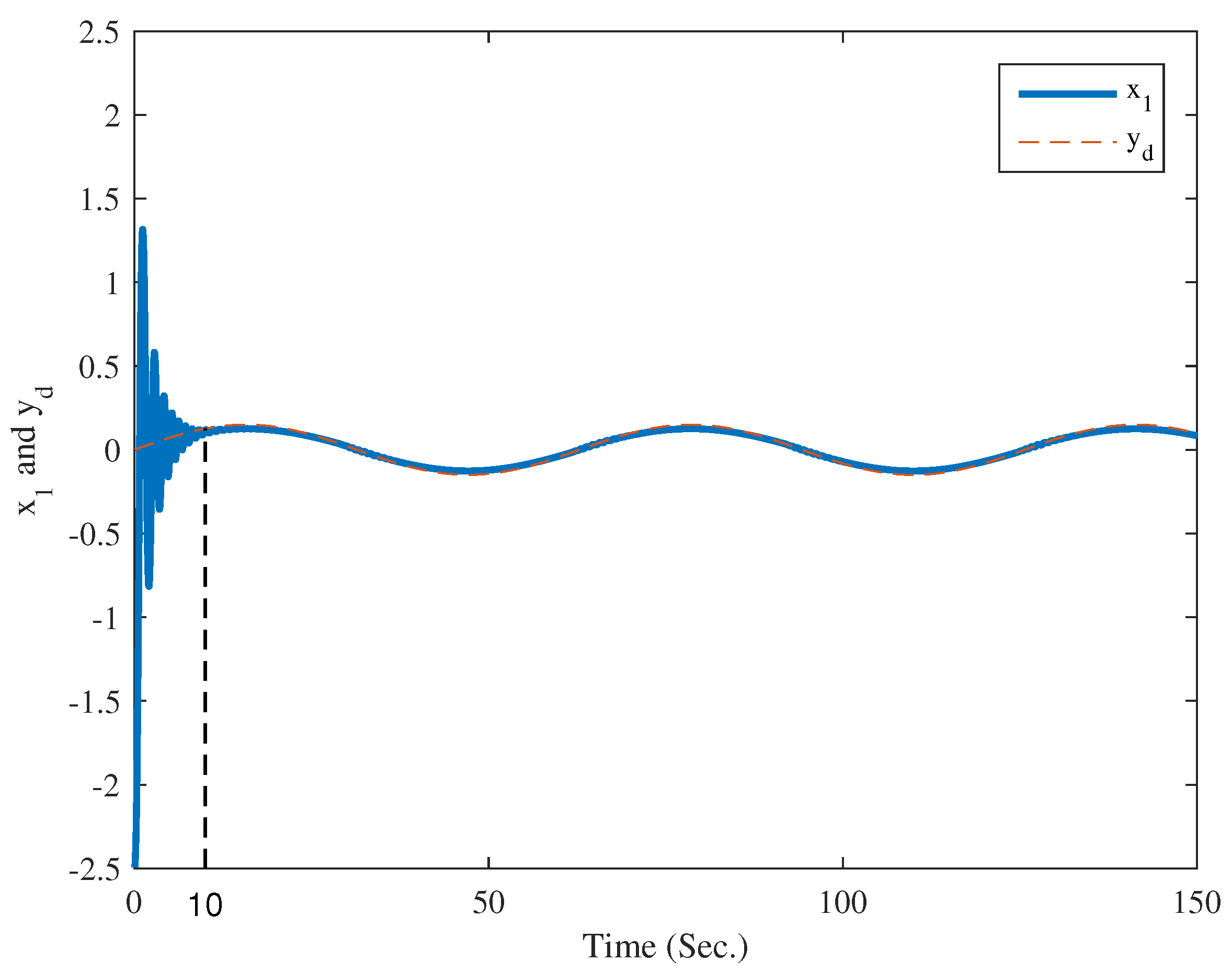
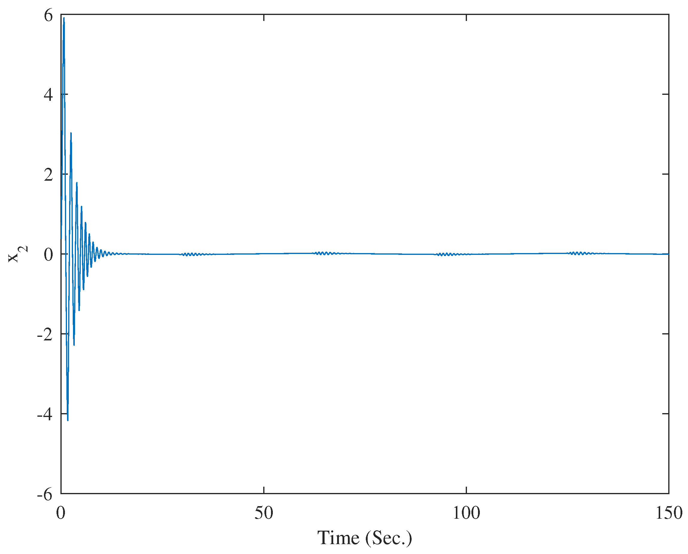
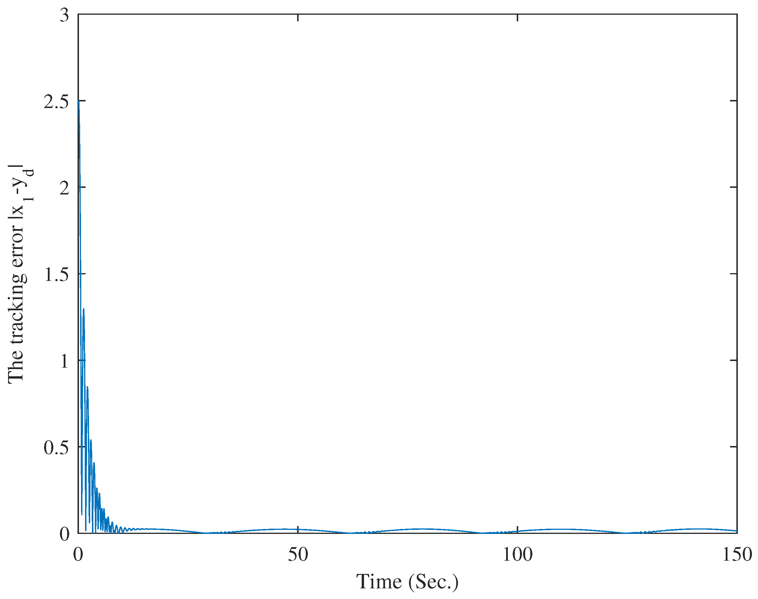
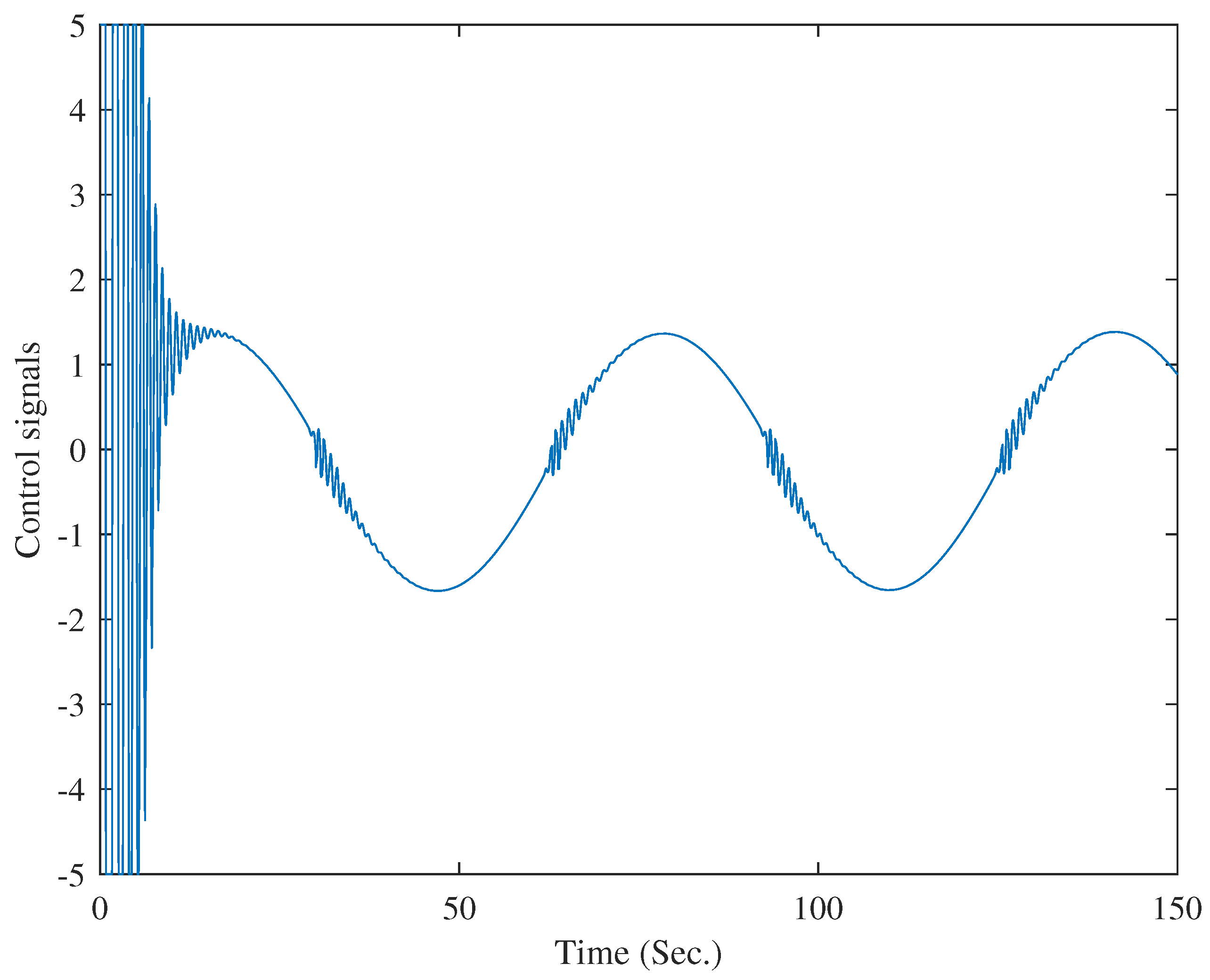
4. Illustrative Examples

To further validate the feasibility of the derived control protocol, a one-line arm dynamics example is utilized, where the system’s dynamic, and the dynamic balance equation are described by

$$\begin{array}{cc}\hfill & \dot{z}=-2z+q^2+0.5\hfill \\ \hfill & M\ddot{q}+N\dot{q}+R\sin \left(q\right)=F+\Delta (q,\dot{q},z\left(q\right),t)\hfill \end{array}$$

(97)

where q and F denote the arm’s position and control input signal, respectively. R = mgL with L = 1 m is the link length, g = 10 N/kg refers to gravitational acceleration, and m = 1 kg refers to the load mass. M = 1 $\mathrm{kg}·{\mathrm{m}}^2$ refers to mechanical inertia. N = 1 N·m·s/rad refers to the coefficient of viscous friction. $\Delta (q,\dot{q},z\left(q\right),t)$ denotes dynamic uncertainty. The dynamic signal is denoted as $\dot{\kappa }=-\kappa +2x_1^4+1$.

Define $x_1=q$, $x_2=\dot{q}$, and ${\Delta }_2(x,z,t)=z{x}_1\cos \left({\mathrm{x}}_2\right)$ then (97) can be expressed as

$$\begin{array}{cc}\hfill \dot{z}=& -2z+x_1^2+0.5\hfill \\ \hfill {\dot{x}}_1& =x_2\hfill \\ \hfill {\dot{x}}_2& =-x_2-10\sin \left(x_1\right)+u+{\Delta }_2(x,z,t)\hfill \\ \hfill y& =x_1\hfill \end{array}$$

(98)

Based on Theorem 1, the finite-time adaptive fuzzy controller (81) is constructed as

$$u=-\frac{{\pi }_1{e}_2{\widehat{\overline{\theta }}}_2^2}{\parallel e_2{\phi }_2^T\left(x_2\right)\parallel {\widehat{\overline{\theta }}}_2+{ϵ}_{21}^{\ast }}-\frac{{\pi }_1{e}_2{\widehat{\overline{\varsigma }}}_2^2}{|e_2|{\widehat{\overline{\varsigma }}}_2+{ϵ}_{22}^{\ast }}-\frac{{\pi }_1}{2}{\mathrm{sgn}}^{\beta }\left(e_2\right)-\frac{1}{4\underline{\hslash }}{e}_2-{\pi }_1{\pi }_2{e}_1$$

(99)

with the adaptation laws, are designed as

$${\dot{\widehat{\overline{\theta }}}}_2=-{\lambda }_{21}{\widehat{\overline{\theta }}}_2+{\lambda }_{21}\parallel e_n{\phi }_2^T\left(x_2\right)\parallel ,{\dot{\widehat{\overline{\varsigma }}}}_2=-{\lambda }_{22}{\widehat{\overline{\varsigma }}}_2+{\lambda }_{22}\left|e_2\right|$$

(100)

The fuzzy the membership functions are defined as ${\mu }_{F^l}(x_1,x_2,\kappa )=\exp [-{(x_1-4+l)}^2/4]\times \exp [-{(x_2-4+l)}^2/16]\times \exp [-{(r-4+l)}^2/16]$, where $l=1,2,\dots ,7$. Furthermore, the fuzzy basic functions can be defined as

$${\phi }^l(x_1,x_2,r)=\frac{{\mu }_{F^l}(x_1,x_2,\kappa )}{{\sum }_{l=1}^7{\mu }_{F^l}(x_1,x_2,\kappa )}$$

(101)

where $\phi ={[{\phi }^1,{\phi }^2,\dots ,{\phi }^7]}^T$.

Case 1. The parameters are chosen as ${\lambda }_{21}=0.002$, ${\lambda }_{22}=0.02$, $\beta =0.3$, $y_d=0.15\sin \left(0.1t\right)$, ${\widehat{\overline{\varsigma }}}_2\left(0\right)=0.01$, ${\widehat{\overline{\theta }}}_2\left(0\right)=0.01$, $ϵ=0.1$, ${\sigma }_2=0.5$, $[x_1\left(0\right),x_2\left(0\right),z\left(0\right),\kappa \left(0\right)]={[-2.5,-0.1,0,0]}^T$, $\hslash \left(t\right)=0.8+0.01\sin \left(0.02t\right)$, and $u_r\left(t\right)=0.1+0.02\cos \left(0.01t\right)$.

For two cases, the simulation results are given in Figure 1, Figure 2, Figure 3, Figure 4, Figure 5, Figure 6, Figure 7, Figure 8, Figure 9 and Figure 10. The response curves of the states $x_1$, $y_d$ and $x_2$ are shown in Figure 1 and Figure 2 for case 1, respectively. The curve of tracking error is shown in Figure 3. It can be seen that the output y can track the reference signal $y_d$ within 10 s for case 1. The curve of control signal is given in Figure 4. The curve of adaptive laws are given in Figure 5. For case 2, the simulation results are given in Figure 6, Figure 7, Figure 8, Figure 9 and Figure 10. The response curves of the states $x_1$, $y_d$ and $x_2$ are given in Figure 6 and Figure 7 for case 2, respectively. It can be seen that the output y can track the reference signal $y_d$ within 11 s for case 2. The curve of tracking error is given in Figure 8. The curve of control signal is given in Figure 9. The curve of adaptive laws are given in Figure 10. Accordingly, the simulation results are given in Figure 1, Figure 2, Figure 3, Figure 4, Figure 5, Figure 6, Figure 7, Figure 8, Figure 9 and Figure 10, where it can be seen that the feasibility of the developed finite-time control strategy in handling unmodeled dynamics and actuator fault problems. Furthermore, the good tracking performance can be ensured within finite-time under the derived adaptive finite-time fuzzy control protocol for the two cases.

Case 2. The parameters are chosen as ${\lambda }_{21}=0.002$, ${\lambda }_{22}=0.02$, $\beta =0.3$, $y_d=0.2\sin \left(0.5t\right)$, ${\widehat{\overline{\varsigma }}}_2\left(0\right)=0.01$, ${\widehat{\overline{\theta }}}_2\left(0\right)=0.01$, $ϵ=0.1$, ${\sigma }_2=0.5$, $[x_1\left(0\right),x_2\left(0\right),z\left(0\right),\kappa \left(0\right)]={[-3,-0.1,0,0]}^T$, $\hslash \left(t\right)=0.9+0.01\cos \left(0.02t\right)$, and $u_r\left(t\right)=0.1+0.02\sin \left(0.01t\right)$.

5. Conclusions

This article examines the issue of adaptive finite-time fuzzy control for nonlinear systems with unmodeled dynamics and actuator faults. The unknown nonlinear terms which are induced during the designer process are modeled by FLSs. The dynamic surface control approach is utilized to design the control scheme to overcome the issue of complexity explosion associated with traditional backstepping. A fuzzy finite-time control scheme has been derived for uncertain nonlinear systems using a finite-time control approach and adaptive backstepping method. Under the derived finite-time control protocol, the resulting system is SGPFS and the tracking error is bounded within finite-time. Moreover, by using the maximal norm of the weight vector estimation method, the communication load was greatly decreased. Illustrative examples have been offered to validate the feasibility of the derived control scheme. Future investigations include considering the fixed-time tracking control for unmodeled dynamical systems under actuator saturation.

References

1. Zhuang, H.; Sun, Q.; Chen, Z.; Zeng, X. Robust adaptive sliding mode attitude control for aircraft systems based on back-stepping method. Aerosp. Sci. Technol. 2021, 118, 107069. [Google Scholar] [CrossRef]
2. Zhang, L.; Ding, H.; Shi, J.; Huang, Y.; Chen, H.; Guo, K.; Li, Q. An adaptive backstepping sliding mode controller to improve vehicle maneuverability and stability via torque vectoring control. IEEE Trans. Veh. Technol. 2020, 69, 2598–2612. [Google Scholar] [CrossRef]
3. Yu, J.; Shi, P.; Zhao, L. Finite-time command filtered backstepping control for a class of nonlinear systems. Automatica 2018, 92, 173–180. [Google Scholar] [CrossRef]
4. Capone, A.; Hirche, S. Backstepping for partially unknown nonlinear systems using Gaussian processes. IEEE Control Syst. Lett. 2019, 3, 416–421. [Google Scholar] [CrossRef]
5. Yan, S.; Gu, Z.; Park, J.H.; Xie, X. Synchronization of delayed fuzzy neural networks with probabilistic communication delay and its application to image encryption. IEEE Trans. Fuzzy Syst. 2023, 31, 930–940. [Google Scholar] [CrossRef]
6. Wang, Y.; Xu, N.; Liu, Y.; Zhao, X. Adaptive fault-tolerant control for switched nonlinear systems based on command filter technique. Appl. Math. Comput. 2021, 392, 125725. [Google Scholar] [CrossRef]
7. Yan, S.; Gu, Z.; Park, J.H.; Xie, X. Distributed-delay-dependent stabilization for networked interval type-2 fuzzy systems with stochastic delay and actuator saturation. IEEE Trans. Syst. Man Cybern. Syst. 2023, 53, 3165–3175. [Google Scholar] [CrossRef]
8. Jiang, S.; Tian, F.; Sun, S.; Liang, W. Integrated guidance and control of guided projectile with multiple constraints based on fuzzy adaptive and dynamic surface. Def. Technol. 2020, 16, 1130–1141. [Google Scholar] [CrossRef]
9. Liu, K.; Wang, R. Antisaturation adaptive fixed-time sliding mode controller design to achieve faster convergence rate and its application. IEEE Trans. Circuits Syst. II Express Briefs 2022, 69, 3555–3559. [Google Scholar] [CrossRef]
10. Yan, S.; Gu, Z.; Park, J.H.; Xie, X. Sampled memory-event-triggered fuzzy load frequency control for wind power systems subject to outliers and transmission delays. IEEE Trans. Cybern. 2022, 1–11. [Google Scholar] [CrossRef]
11. Liu, K.; Wang, R.; Zheng, S.; Dong, S.; Sun, G. Fixed-time disturbance observer-based robust fault-tolerant tracking control for uncertain quadrotor UAV subject to input delay. Nonlinear Dyn. 2022, 107, 2363–2390. [Google Scholar] [CrossRef]
12. von Ellenrieder, K.D. Dynamic surface control of trajectory tracking marine vehicles with actuator magnitude and rate limits. Automatica 2019, 105, 433–442. [Google Scholar] [CrossRef]
13. Li, Y.; Li, K.; Tong, S. Finite-time adaptive fuzzy output feedback dynamic surface control for MIMO nonstrict feedback systems. IEEE Trans. Fuzzy Syst. 2018, 27, 96–110. [Google Scholar] [CrossRef]
14. Ma, H.; Liang, H.; Zhou, Q.; Ahn, C.K. Adaptive dynamic surface control design for uncertain nonlinear strict-feedback systems with unknown control direction and disturbances. IEEE Trans. Syst. Man Cybern. Syst. 2018, 49, 506–515. [Google Scholar] [CrossRef]
15. Li, H.; Wu, Y.; Chen, M. Adaptive fault-tolerant tracking control for discrete-time multiagent systems via reinforcement learning algorithm. IEEE Trans. Cybern. 2020, 51, 1163–1174. [Google Scholar] [CrossRef] [PubMed]
16. Hua, C.; Li, Z.; Li, K.; Chen, S.; Sun, J. Distributed control for uncertain nonlinear multiagent systems subject to hybrid faults. Int. J. Control. Autom. Syst. 2020, 18, 2589–2598. [Google Scholar] [CrossRef]
17. Dong, G.; Ren, H.; Yao, D.; Li, H.; Lu, R. Prescribed performance consensus fuzzy control of multiagent systems with nonaffine nonlinear faults. IEEE Trans. Fuzzy Syst. 2020, 29, 3936–3946. [Google Scholar] [CrossRef]
18. Du, H.; Wen, G.; Cheng, Y.; Lü, J. Design and implementation of bounded finite-time control algorithm for speed regulation of permanent magnet synchronous motor. IEEE Trans. Ind. Electron. 2020, 68, 2417–2426. [Google Scholar] [CrossRef]
19. Lei, R.; Chen, L. Finite-time tracking control and vibration suppression based on the concept of virtual control force for flexible two-link space robot. Def. Technol. 2021, 17, 874–883. [Google Scholar] [CrossRef]
20. Song, C.; Yu, J.; Zhao, L.; Ma, Y. Full-state constraints-based neuroadaptive finite-time control for induction motor drive systems with iron losses. Int. J. Control Autom. Syst. 2022, 20, 637–647. [Google Scholar] [CrossRef]
21. Liu, K.; Wang, Y.; Ji, H.; Wang, S. Adaptive saturated tracking control for spacecraft proximity operations via integral terminal sliding mode technique. Int. J. Robust Nonlinear Control 2021, 31, 9372–9396. [Google Scholar] [CrossRef]
22. Li, S.; Ahn, C.K.; Xiang, Z. Command-filter-based adaptive fuzzy finite-time control for switched nonlinear systems using state-dependent switching method. IEEE Trans. Fuzzy Syst. 2020, 29, 833–845. [Google Scholar] [CrossRef]
23. Sun, W.; Wu, Y.; Sun, Z. Command filter-based finite-time adaptive fuzzy control for uncertain nonlinear systems with prescribed performance. IEEE Trans. Fuzzy Syst. 2020, 28, 3161–3170. [Google Scholar] [CrossRef]
24. Lv, W. Finite time adaptive fault-tolerant control for nonlinear MIMO systems with actuator faults. Int. J. Control Autom. Syst. 2022, 20, 99–108. [Google Scholar] [CrossRef]
25. Nguyen, N.P.; Mung, N.X.; Ha, L.N.N.T.; Huynh, T.T.; Hong, S.K. Finite-time attitude fault tolerant control of quadcopter system via neural networks. Mathematics 2020, 8, 1541. [Google Scholar] [CrossRef]
26. Wang, Z.; Yuan, Y.; Yang, H. Adaptive fuzzy tracking control for strict-feedback Markov jumping nonlinear systems with actuator failures and unmodeled dynamics. IEEE Trans. Cybern. 2018, 50, 126–139. [Google Scholar] [CrossRef] [PubMed]
27. Jing, Y.; Yang, G. Fuzzy adaptive fault-tolerant control for uncertain nonlinear systems with unknown dead-zone and unmodeled dynamics. IEEE Trans. Fuzzy Syst. 2019, 27, 2265–2278. [Google Scholar] [CrossRef]
28. Yang, Y.; Tang, L.; Zou, W.; Ding, D.-W.; Ahn, C.K. A unified fixed-time framework of adaptive fuzzy controller design for unmodeled dynamical systems with intermittent feedback. Inf. Sci. 2022, 611, 628–648. [Google Scholar] [CrossRef]
29. Wang, J.; Tian, Y.; Hua, L.; Shi, K.; Zhong, S.; Wen, S. New results on finite-time synchronization control of chaotic memristor-based inertial neural networks with time-varying delays. Mathematics 2023, 11, 684. [Google Scholar] [CrossRef]
30. Li, Y.; Liang, H. Robust finite-time control algorithm based on dynamic sliding mode for satellite attitude maneuver. Mathematics 2022, 10, 111. [Google Scholar] [CrossRef]
31. Hardy, H.; Littlewood, E.; Polya, J. Inequalities; Cambridge University Press: Cambridge, UK, 1995. [Google Scholar]
32. Deng, H.; Krstic, M. Output-feedback stochastic nonlinear stabilization. IEEE Trans. Autom. Control 1999, 44, 328–333. [Google Scholar] [CrossRef]
33. Wang, F.; Chen, B.; Liu, X.; Lin, C. Finite-time adaptive fuzzy tracking control design for nonlinear systems. IEEE Trans. Fuzzy Syst. 2017, 26, 1207–1216. [Google Scholar] [CrossRef]
34. Meng, B.; Liu, W.; Qi, X. Disturbance and state observer-based adaptive finite-time control for quantized nonlinear systems with unknown control directions. J. Frankl. Inst. 2022, 359, 2906–2931. [Google Scholar] [CrossRef]
35. Jiang, Z.; Praly, L. Design of robust adaptive controllers for nonlinear systems with dynamic uncertainties. Automatica 1998, 34, 825–840. [Google Scholar] [CrossRef]
36. Deng, C.; Yang, G. Distributed adaptive fuzzy control for nonlinear multiagent systems under directed graphs. IEEE Trans. Fuzzy Syst. 2017, 26, 1356–1366. [Google Scholar]
37. Liu, K.; Wang, R. Antisaturation command filtered backstepping control-based disturbance rejection for a quadarotor UAV. IEEE Trans. Circuits Syst. II Express Briefs 2021, 68, 3577–3581. [Google Scholar] [CrossRef]
38. Kong, L.; Yu, X.; Zhang, S. Neuro-learning-based adaptive control for state-constrained strict-feedback systems with unknown control direction. ISA Trans. 2021, 112, 12–22. [Google Scholar] [CrossRef]
Figure 1. The curves of the state x 1 and y d in case 1.
Mathematics 11 02193 g001
Figure 2. The curve of the state x 2 in case 1.
Mathematics 11 02193 g002
Figure 3. The curves of tracking error | x 1 y d | in case 1.
Mathematics 11 02193 g003
Figure 4. The curve of control signal in case 1.
Mathematics 11 02193 g004
Figure 5. The curves of adaptive laws θ ¯ ^ 2 and ς ¯ ^ 2 in case 1.
Mathematics 11 02193 g005
Figure 6. The curves of the state x 1 and y d in case 2.
Mathematics 11 02193 g006
Figure 7. The curve of the state x 2 in case 2.
Mathematics 11 02193 g007
Figure 8. The curves of tracking error | x 1 y d | in case 2.
Mathematics 11 02193 g008
Figure 9. The curve of control signal in case 2.
Mathematics 11 02193 g009
Figure 10. The curves of adaptive laws θ ¯ ^ 2 and ς ¯ ^ 2 in case 2.
Mathematics 11 02193 g010
Disclaimer/Publisher’s Note: The statements, opinions and data contained in all publications are solely those of the individual author(s) and contributor(s) and not of MDPI and/or the editor(s). MDPI and/or the editor(s) disclaim responsibility for any injury to people or property resulting from any ideas, methods, instructions or products referred to in the content.