Article

The Gibbons, Ross, and Shanken Test for Portfolio Efficiency: A Note Based on Its Trigonometric Properties

Maine Business School, University of Maine, Orono, ME 04469, USA
Mathematics 2023, 11(9), 2198; https://doi.org/10.3390/math11092198
Submission received: 10 April 2023 / Revised: 29 April 2023 / Accepted: 2 May 2023 / Published: 6 May 2023

Abstract

:
This study is intended as a note and provides an extension to a much-used and established test for portfolio efficiency, the Gibbons, Ross, and Shanken GRS-Wald test. Tests devised to measure portfolio efficiency are crucial to the theoretical issues related to CAPM (Capital Asset Pricing Model) testing and have applications for the fund manager who seeks to rank portfolio performance. This study looks at the GRS-Wald test for portfolio efficiency and extends it to make it visually more interpretive without any loss of generality in its structure. The geometrically recast statistic draws upon the trigonometric properties of a portfolio in the mean-variance space and a mathematical proof of the equivalence of the two statistics is provided. The GRS-Wald test is a widely used statistic in studies addressing the issue of portfolio efficiency and CAPM deviations. A simulation demonstrates the use of the recast GRS-Wald test in testing for the mean-variance efficiency of a test portfolio. The study also provides a table of the GRS-Wald test, based on a range of mean-variance locations (cosine of portfolio angles) at which the test portfolio and the efficient market portfolio can be placed.

1. Introduction

The GRS-Wald test statistic, Gibbons, Ross, and Shanken [1] (hereinafter the GRS-W test or the GRS-test, or the GRS-statistic), is a widely used statistic to test for portfolio efficiency. This study is a note and provides an extension to the GRS test, which is also used to study the CAPM (Capital Asset Pricing Model) deviations (Galea, Curci, and Molina [2]; Fama and French [3]). The test is recast in a form that is visually more intuitive (geometrically), while maintaining its original structure. At the same time, the recast statistic does not suffer from any loss of generality or rigor in its structure. The recast statistic draws upon the trigonometric properties (Gustafson [4,5], Rodriguez [6]) of a portfolio in the mean-variance space, and a mathematical proof of the equivalence of the two statistics is provided. A simulation is also employed to demonstrate the use of the recast GRS statistic in testing for the mean-variance efficiency of a test portfolio, and a table of values, based on a range of angles, spanning the various points on the mean-variance spectrum is presented (Appendix A.3). The GRS~W test is a multivariate statistic for testing the mean-variance efficiency of a portfolio, it also has a geometric interpretation. The statistic tests for the efficiency of proxies used for the market portfolio and enables them to address issues related to the critique by Roll [7] regarding the validity of the empirical testing procedures on the CAPM (Capital Asset Pricing Model, Chen [8]. Testing for the efficiency of the proxies used is important because, “if the proxy is not a valid surrogate, then as tests of the CAPM the existing empirical investigations are somewhat beside the point” (Gibbons, Ross, and Shanken [1]). Hu et al. [9] solved the portfolio optimization problem of the mean-variance model (as used in the GRS-test) by developing an interactive multi-criterion, self-learning system that does not require an a priori assumption of the agent’s utility preference structure.

2. The Gibbons, Ross, and Shanken Test Statistic and Its Relevance

Bodnar and Schmid [10] speak of the GRS test as an exact F-test for the efficiency of a given portfolio which has become a fundamental test in portfolio theory. Cueto, Grané, and Caascos [11], deploy the GRS test to assess the ability of a multifactorial risk model to explain excess returns, by determining if the regression intercepts are jointly zero, α1 = α2 = … = αn = 0. Ryan et al. [12], utilizing the GRS-test, look at the average value of absolute intercepts, αi = 0 to test whether the regression intercepts are jointly equal to zero, with the idea being that the intercept is indistinguishable from zero if an asset pricing model completely captures the expected returns (in which case the portfolio is efficient). Suarez and Alonso-Conde [13] looked at an entropy-based decomposition that captures the divergence between the factor-mimicking portfolio and the minimum-variance pricing kernel as distinct from quadratic test statistics, such as the GRS-test (determined as a function of pricing errors). Solórzano-Taborga et al. [14], utilize the GRS test for identifying restrictions (they termed ‘efficiency factor’) to test the null of asset pricing errors equaling zero. Barillas et al. [15] utilized the GRS test to accommodate the comparison of non-nested models as in a squared Sharpe-ratio (Sharpe [16]). Kamstra and Shi [17] rigorously generalized the Sharpe ratio-based interpretation of the GRS test to the multiple portfolio case but also suggested modifications to it when extended to multiple factors.
It may be noted that the GRS test does not accommodate short-selling restrictions (Fletcher [18]). Vigo-Pereira and Laurini [19] stated that for the GRS test to be effective the error terms have to be i.i.d N(0,1), normally distributed ~ N(μ, σ2); f x = 1 σ 2 π e 1 2 x μ σ 2 , homoscedastic with the diagonal elements jj and kk of two var-cov matrices A and B being equal, A j j = B k k , j = k , and uncorrelated ρ ϵ j , ϵ k = 0 . Kamstra and Shi [17] asserted that the GRS statistic can lead to higher failure rates especially when the returned model has K-factors, K > 1 and N-assets, N < N*; “the bias to over-reject is non-negligible in small samples”. The short-selling constraint prevents the replication of an investible benchmark index, thus invoking Roll’s Critique [7] of whether the benchmark is representative of the test portfolio. However, tests of mean-variance efficiency with no short sales constraints have been proposed by Basak et al. [20]. Kim and Robinson [21] also point out that perfect efficiency cannot exist in practice and that it would be unrealistic that all intercept values were jointly and exactly zero, hence they introduce an interval-based hypothesis testing and get lower rejection rates with the GRS-test.
Shanken [22] provided an exhaustive review of 23 statistical methods that have been used in testing mean-variance portfolio efficiency. Kamstra and Shi [17] posited that “the Gibbons, Ross, and Shanken ([1], GRS) test of mean-variance efficiency of asset returns is the gold standard of empirical asset pricing, used by virtually every paper in the literature exploring empirical asset pricing models. Not only is it used to establish if an asset pricing model can account for expected returns of a set of test assets, but the GRS test is also used to rank models for relatively superior performance, that is, which model produces the lower GRS statistic (see, for instance, Fama and French [3])”. Essentially, this is done by testing for the intercepts on a multifactor risk model to be jointly zero, indicating that there is no excess return to the factor loadings. Cueto et al. [11], deploy the GRS test to assess the ability of a multifactorial risk model to explain excess returns, by determining if the regression intercepts are jointly zero, α1 = α2 = … = αn = 0. Ryan et al. [12], utilizing the GRS test, looked at the average value of absolute intercepts, αi = 0 to test whether the regression intercepts are jointly equal to zero, with the idea being that the intercept is indistinguishable from zero if an asset pricing model completely captures the expected returns (in which case the portfolio is efficient). It can be surmised that there is a substantive link between the GRS test, and portfolio performance evaluation and that it has been well-researched. This paper abstracts from those empirical tests and seeks to provide a trigonometric interpretation of the GRS test.
MacKinlay [23] discriminated between the risk-based and the non-risk-based explanations of CAPM deviations and indicates that models that base their explanations on the need for additional risk factors may be making premature conclusions (Roll and Ross [24]. He further adds that on an ex ante basis, “CAPM deviations due to missing risk factors will be very difficult to statistically detect”. The main point of his study is that the adoption of empirically developed multifactor models is not the answer to observed CAPM deviations. His study utilized the GRS test to detect CAPM deviations on an ex ante basis. Using a 342-month time series of excess returns for 32 portfolios (25 stock and 7 bond portfolios) as the dependent variable, with market excess returns being the independent variable, he tested for the null hypothesis that the intercept on the CAPM is zero. He finds that on an ex ante basis, it is more probable that the deviations are better explained by non-risk-based alternatives than by additional risk-based alternatives. This is inferred from the degree of overlap the alternative distributions have over the GRS-test statistic MacKinlay [23]. For purposes of comparing a risk-based model with a non-risk-based alternative, MacKinlay [23] stated, “the zero-intercept test can be very useful since the distributions of the test statistic for these alternatives have little overlap”.
Zhou [25] stated, “the GRS test has rich economic interpretations and attractive statistical properties … the GRS test is fundamental for testing MV (mean-variance) efficiency under normality.” He uses the statistic and rejects the MV efficiency on the CRSP (Center for Research in Security Prices, WRDS [26]; Agrrawal [27]) value-weighted stock index for three of the six consecutive ten-year sub-periods from 1926 to 1986 besides rejecting the normality assumption of the data at the same time. Zhou [25] conducts the zero-intercept test on the CAPM under the normality as well as the alternative (elliptical) distribution assumption and uses the values of the GRS statistic to calculate the p-values (level of significance). Bodnar et al. [28] also mentioned that Zhou [25] extended the findings of Gibbons et al. [1] by applying their GRS test of the validity of the CAPM to elliptically distributed returns. For the alternative distributions of excess returns, he reported that the p-values for five of the six sub-periods from 1926–1976 exceed 5% and are larger than the p-values under the normality assumption (Table V, Panel B, p. 1938, Zhou [25]). This prevents the rejection of the null hypothesis (zero-intercept on the excess return form of the CAPM) for the period under study. The Zhou [25] paper thus introduces a refinement to the GRS-test by way of testing the implications of the GRS-test to alternative distributions and cautions that “empirical studies that ignore the nonnormality are likely to over reject the theory being tested”. At the same time, it brings out the appeal of the GRS test to situations that call for the testing of portfolios.
The Fama and French [29] study used 32 portfolios over 342 monthly observations to arrive at the GRS-test F-value of 1.91 (for the single factor case with excess market returns as the sole independent factor). The study rejects the null of a zero-intercept at the 99.6% level (Fama and French [29]). Their lowest F-statistic (closer to zero, implying higher efficiency) has a value of 1.56 and rejects the null at the 96.1% level; in this case, their model is the three-factor stock market model. Despite its ‘marginal rejection’ in the F-tests, they feel “the three-factor model does a good job on the cross-section of stock returns”. The five-factor (3 stock and 2 bond market) model has an F-value of 1.66 and rejects the null at the 97.5% level, which is lower than the three other scenarios. This prompts them to conclude that “the five-factor regressions provide the best model for returns on bonds and stocks”. A look at the p-values for the overall regressions clearly shows that the null of a zero-intercept is rejected at least at the 96.1% level (which is the lowest on the table referred to above). Evidently, the Fama and French [29] study makes a strong case for multi-factor risk-based alternates to the univariate proposition of the CAPM. Hou, Karolyi, and Kho [30] used the GRS-test statistic for their country, industry, and characteristic-based global test portfolios. Ehsani and Linnainmaa [31] utilized the GRS test to see if factor momentum contributes to the returns of cross-sectional momentum strategies and test the null hypothesis of the alphas being jointly zero. This note provides an extension/recharacterization of the GRS test with the objective of giving it a geometrical interpretation and making its implementation easier.

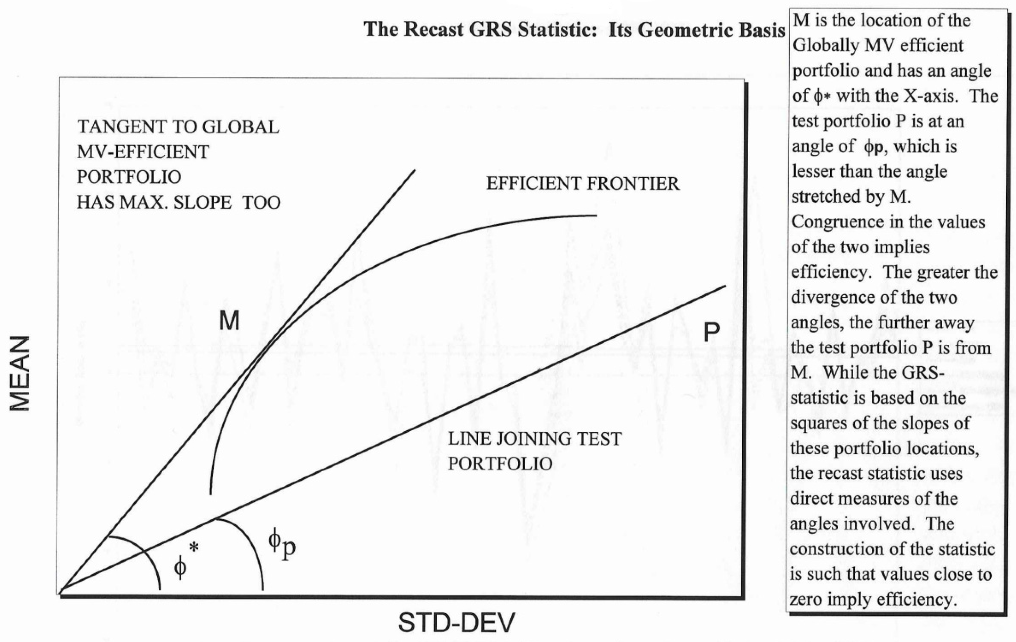
3. Suggested Recharacterization of the GRS-Statistic

Gibbons, Ross, and Shanken [1] devised a statistic to test for the MV efficiency of any particular portfolio. Their motivation was to examine the MV efficiency of market proxies used in CAPM testing, especially given the equivalence of the CAPM to MV efficiency of the market. They derived an exact form test and examined its sensitivity to the choice of the portfolio and the number of assets used to derive the MV efficiency frontier (Merton [32]). They found that “conclusions regarding the efficiency of a given index can be altered by the type of assets used to construct the ex post frontier”. Their tests reject the efficiency of the CRSP value-weighted (VW) index but do not reject the efficiency of the CRSP equal-weighted (EW) index, and utilized monthly data over the period from 1931–1965. They also provided a geometrical (Gomez-Deniz et al. [33]; Danko and Soltés [34]) interpretation of their test in “the mean-standard deviation space of portfolio theory”, something that this study attempted to extend.
The GRS statistic measures the distance, in mean-standard deviation space, between a test portfolio (market index), and a tangency portfolio (on the efficient frontier) and returns a value, which is then used to assess the relative efficiency of the portfolio under consideration. The GRS test statistic, also called the GRS-W, statistic is as follows:
W = 1 + θ ^ * 2 1 + θ ^ p 2 2 1 ψ 2 1
and θ ^ * is the Sharpe measure of the ex post efficient portfolio (ratio of expected excess return to the standard deviation of the excess return), and θ ^ p is the Sharpe measure of the test portfolio. Note that Ψ cannot be less than one since θ ^ * is the slope of the ex post frontier and is based on all the assets in the test (including the test portfolio p). To accept the efficiency of the test portfolio, Ψ 2 should be close to 1. Larger numerical values of Ψ 2 imply portfolio inefficiency (MacKinlay et al. [35]) arising out of the increased distance between the test portfolio and the global MV efficient portfolio on the frontier ( W = Ψ 2 1 0 implies efficiency). In other words, for values of W close to zero, the test portfolio cannot be called inefficient.
The null hypotheses of a zero intercept on the excess-return form of the CAPM can be rejected when the value of W is greater than the F-statistic value with degrees of freedom N and (T-N-1), where N is the number of assets and T is the number of time series observations on the underlying asset returns.
It may be noticed that the above statistic involves the prior calculation of the slopes of the tangent to the efficient frontier and the segment joining the test portfolio to the origin. Additionally, θ is a slope measure ( θ r ¯ / σ ) with excess return ( r ¯ ) and standard deviation of return (σ). The simplification of this approach involves the direct use of the angles stretched by the two lines, and could perhaps aid in a more visually intuitive use of the GRS test statistic. The suggested modification on the original form of the GRS statistic is as follows.
Let ϕ* be the angle between tangent OM and the X-axis (Figure 1), and ϕ p be the angle between the segment OP and the X-axis.
Then, we can recast the GRS-W statistic as W ~ , where:
W ~ = cos ϕ p cos ϕ * 2 1
If W ~ = Ψ 2 1 0 , we cannot reject Ho (which indicates that the test portfolio P is efficient), and ϕ* is the angle between the tangency portfolio and the X-axis:
sec ϕ * sec ϕ p 2 1
and ϕp is the angle between the test portfolio and the X-axis,
sec 2 ϕ * sec 2 ϕ p 2 1
1 + t a n 2 ϕ * 1 + t a n 2 ϕ p 2 1
1 + θ ^ * 2 1 + θ ^ p 2 2 1
where θ is a slope measure ( θ r ¯ / σ ); tan(ϕ) = θ, which is the exact form of W ˜ , the original GRS-W test statistic (Gibbons, Ross, and Shanken [1]).
The return vectors ri ≡ xi generate a s c a l a r   v a r i a n c e   p r o d u c t   x 1 . x 2 v a r x .
where   correlation   ρ x 1 x 2 = c o v x 1 x 2 σ x 1 σ x 2
= x 1 · x 2 η 1 x 1 η 1 1 x 2 η 1 1         f o r   s c a l e d   r e t u r n s   x 1 , x 2   a n d   η   o b s e r v a t i o n s . W h e r e   t h e   s q u a r e d   l e n g t h   o f   v e c t o r   x 1 , x 2   i s : x 1 2 = a 1 2 + a 2 2 + a n 2 2 x 2 2 = b 1 2 + b 2 2 + b n 2 2 P r o d u c t   o f   v e c t o r s   A , B   i s   a . b = a · b   c o s ( α ) a = a 1 , a 2 a n x 1 b = b 1 , b 2 b n x 2
Note that P denotes the test portfolio, so it lies on or below the frontier (above it would violate the budget constraint and is hence infeasible). The proof involves the use of some basic axioms of trigonometry ( s u c h   a s   1 + t a n 2 θ = s e c 2 θ ), and displays the equivalence of the original form of the GRS test to its recast form. This is important because the recast GRS-W statistic leaves the numerical value of the test unchanged while at the same time providing a geometrical interpretation (the closer the test portfolio line is to the tangency portfolio line, the more efficient the test portfolio is) and computational ease. In that sense, there is no structural change to the original GRS-W test; it is just extended to provide a geometric and trigonometric interpretation.
A calculator with trigonometric functions can easily compute the W ~ statistic, thus giving it a quick-and-ready status. It also obviates the need to calculate the length of the hypotenuse for the two points under consideration, and all that is needed is the value of the angles between the two lines and the X-axis. This quick-and-ready W ~ statistic that measures the efficiency of a portfolio can be useful for professional fund manager presentations and instruction on the MV efficiency criterion. At the same time the recast statistic W ~ does not suffer from any loss of generality or rigor in its structure. The study suggests this recast portfolio efficiency test statistic as an extension and not a replacement for the GRS-W test statistic.

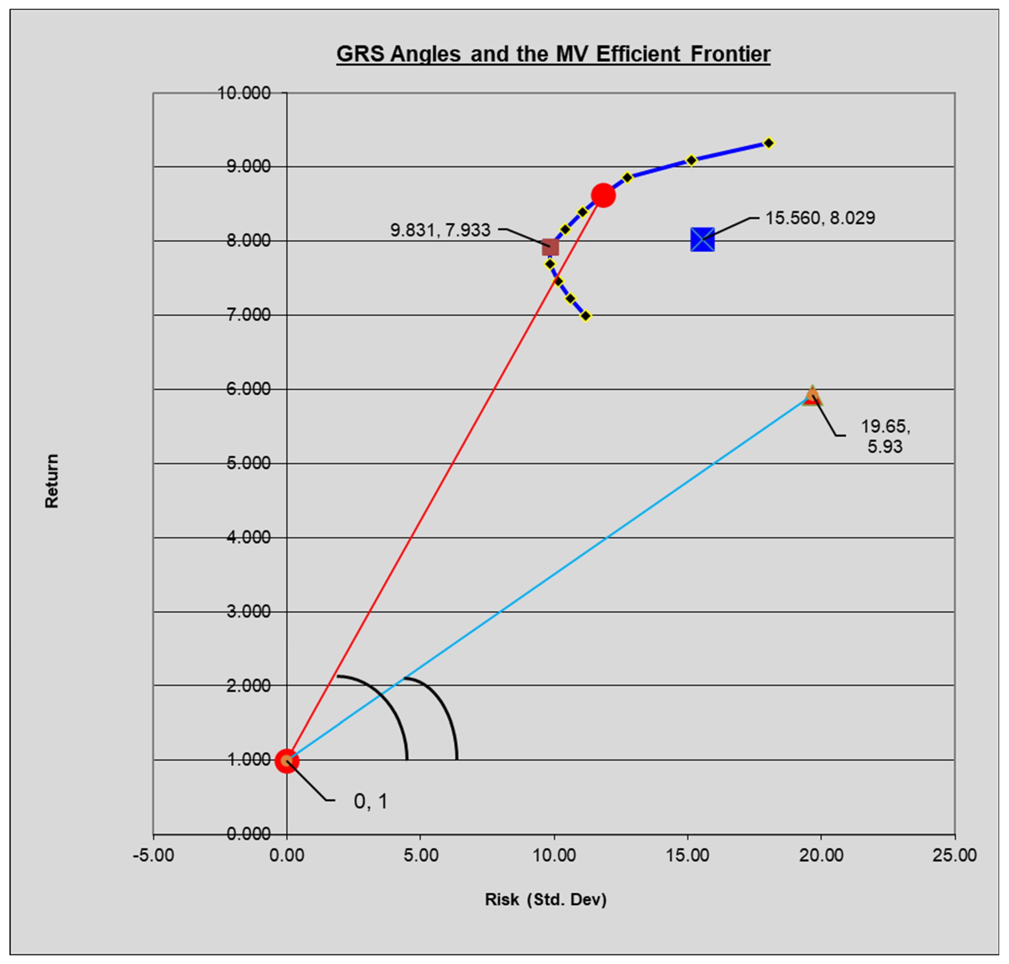
4. A Simulated Efficient Frontier and a Test of Portfolio Efficiency

This section delves into the mechanics of tracing out an efficient MV frontier and identifying the relative location of the global MV-efficient portfolio. Thereafter, the location of an EW portfolio having the same return distribution as those of the assets employed in the formation of the efficient frontier is noted and its efficiency is tested using the recast GRS statistic. This enables us to improve on the simple eyeballing technique employed in testing the efficiency of a test portfolio used in the works of Roll and Ross [24].
The simulations begin with an initial set of five assets i whose returns are randomly generated under the assumption of normality. More specifically, the distribution specified is a Gaussian distribution of the return (r) random variable x, with mean and standard deviation ~ N(μ, σ2) and having a p.d.f.:
f x = 1 σ 2 π e 1 2 x μ σ 2
where μi was successively set at 0, 2, 4, 6, 8, 10 and σi was set at 0, 5, 10, 15, 20, 25.
Now, the problem reduces to one of minimizing the variance of a portfolio subject to a target rate of return and a budget constraint. The MV portfolio selection problem is one where the investor seeks to minimize the portfolio variance subject to the budget and target return constraint. A short selling, Black [36] non-negativity constraint is optional, depending on the model (Buckle [37] utilized a bivariate normal distribution due to option payoffs). Simply stated, the problem is to
M i n i m i z e σ 2 ( x ) = x T Σ x s u b j e c t t o , x T e = 1 w h e r e e T = [ 1 ,   1 , 1 ] x T μ = μ p a n d x o ( o p t i o n a l )
where, μ and x are n-vectors composed of asset rates of return and portfolio weights respectively:
Σ is an n x n positive-definite non-singular covariance matrix;
e is a unit vector;
μ p is a scalar equal to the targeted portfolio return;
And x  0 is the short-selling constraint.
The equivalent Parametric Quadratic Programming (PQP) problem (Best and Grauer [38,39]) is
M a x x T μ x T Σ x 2 A x γ
where, A is an m × n constraint matrix, γ an m × 1 vector, for a given var-cov matrix Σ and Σ = σ 11 σ 22 s i n 2 α , where σ is the standard deviation of returns; it is well known that Generalized Variance is
G V = x 1 x 2 sin α η 1 2
for η observations, with α, the angle between the vectors x1 and x2 respectively. Another approach, called the Risk parity based allocation approaches does not require an estimate of the return vectors. Lee [40] outlined a process that is elaborated in Appendix A.4).
The solution involves the use of the Kuhn-Tucker [41] conditions (please see Appendix A.1 for the K-T conditions) to arrive at a global optimum portfolio (it is a saddle point where the variance is minimized in one plane and the mean return is maximized in the other).
However, computational solutions that hinge on algorithms, are developed for the solution of non-linear quadratic programming situations. Greene [42] reviewed some commonly used NLP algorithms and stated that the quasi-Newton algorithms belong to a ”very effective class of algorithms that eliminates second derivatives altogether and has excellent convergence properties, even for ill-behaved problems”. The results of this optimization can be seen in Table 1, which gives us the GRS-test values for a range of portfolio returns and standard deviations (Appendix A.2). Following Roll and Ross [24] and Shefrin and Statman [43], feasible portfolios away from the tangency portfolio will plot below the efficient frontier (infeasible above the frontier).
The plot of the efficient frontier (Figure 2) shows that this is indeed the case. The inefficient EW portfolio lies inside the frontier and considerably away from the global MV efficient portfolio. The global tangency portfolio (M) produces the highest return per unit of risk amongst all other efficient portfolios; in other words, it generates the highest value of the Sharpe ratio [16] measure for portfolio performance.
Glabadanidis [44] proposed a new finite sample mean-variance efficiency test based on the risk reduction of the global minimum variance (GMV) portfolio, which he found has a straightforward geometric and portfolio interpretation and complements the celebrated GRS-test well Notice that M is tangential to a line emanating from the origin and has the property of maximizing the angle formed between the axis that measures risk and the line through the origin. Any other portfolio on or below the frontier will generate an angle that will be lesser in value. The study noted the significance of this property of the global MV efficient portfolio and employed this unique characteristic to devise a formal test for portfolio efficiency using the values of the angles formed by the test and the global MV efficient portfolio with the risk axis. While it may be visually appealing to comment on the efficiency of a test portfolio based on its distance from the global MV efficient portfolio, a mathematically precise test conveys the information with greater clarity and conviction.
The first step in arriving at the values of the recast GRS statistic requires the precise calculation of the “portfolio angles”, since these values form an integral part of the test of portfolio efficiency. The change in the gradient of the “W stat” as (x, y) changes is shown in Figure 3; with the X-coordinate representing return and the Y-coordinate measuring the standard deviation on the portfolio, an application of the Pythagorean theorem allows us to arrive at the values of the angles created by such coordinates in the Cartesian plane.
Stated simply, the theorem states that for any right-angled triangle, the value of the hypotenuse-squared (h2) equals the sum of the values of the perpendicular (p2)-squared and the base-squared (b2), i.e., h2 = p2 + b2. For example, for the coordinates of the EW portfolio and the M portfolio (8, 4.67) and (12, 5.05); the values of the angles stretched by the two given coordinates are found as follows:
h ( ϕ p ) = 4.67 2 + 8 2 = 9.263
where   h ( ϕ p )   is   the   hypotenuse   of   the   right   angled   triangle   formed   with   two known   vertices   at   ( 0 , 0 )   and   ( 4 . 67 , 8 ) . cos ϕ p = b / h = ( 4.67 / 9.263 ) = 0.5042 cos 1 0.5042 = 59.717 o ϕ p = 59.717 o Similarly ,   h ( ϕ * ) = 13 . 019 ϕ * = 67.176 o , the   angle   stretched   by   the   global   min - var   portfolio   M . Recalling that the GRS-statistic also called the GRS-W statistic is
W = 1 + θ ^ * 2 1 + θ ^ p 2 2 1 ψ 2 1
(For values of W close to zero, the test portfolio cannot be called inefficient).
It has been shown that it can be recast in the following form:
W ˜ = cos ϕ p cos ϕ * 2 1 And if W ˜ 0 , we cannot reject the efficiency of the test portfolio p .
Using the values found above we can see that W ˜ = 0.689 which is not close to zero, thus implying inefficiency of the test portfolio p, which, in this case, is the EW portfolio comprised of the five asset universe. Is the value of the recast GRS statistic W ˜ equal to the original form value of W? The original form of the GRS construction θ is the slope of a line and the Sharpe measure for the ex post price of risk. The GRS test defines θ r ¯ / σ as the Sharpe measure with excess return ( r ¯ ) and standard deviation of return (σ). On a more specific basis, θ ^ * is the Sharpe measure of the ex post efficient portfolio (ratio of expected excess return to the standard deviation of the excess return), while θ ^ p is the Sharpe measure of the test portfolio. Jurdi [45] and Agrrawal et al. [46] note that investors rely on the ex-post performance of portfolios to assess the economic utility of their asset allocation and guide the portfolio rebalancing decision. Bazhutov et al. [47] further note that no market portfolio is clearly defined in CAPM testing. The coordinates of the EW test portfolio (P) and the M portfolio are (8, 4.67) and (12, 5.05), respectively, with the X-coordinate representing return and the Y-coordinate measuring the standard deviation on the portfolio. Then,
W = 1 + θ ^ * 2 1 + θ ^ p 2 2 1 = 1 + 12 5.05 2 1 + 8 4.67 2 2 1 = 0.689 = W ^
The above mentioned demonstration shows the equality of the two statistics when actual numbers are used. The recast approach, however, involves the direct use of the angles stretched by the two lines in the hope that this could perhaps aid in a visually more intuitive use of the GRS statistic.
The GRS statistic also measures the distance, in mean-standard deviation space, between a test portfolio (market index) and a tangency portfolio (on the efficient frontier) and returns a value which is then used to assess the relative efficiency of the portfolio under consideration. The GRS statistic denoted by GRS-W is given as
W = 1 + θ ^ * 2 1 + θ ^ p 2 2 1 ψ 2 1
where, θ ^ * is the Sharpe measure of the ex post efficient portfolio (ratio of expected excess return to the standard deviation of the excess return), and θ ^ p is the Sharpe measure of the test portfolio. Essentially, θ is a slope measure ( θ r ¯ / σ ) with excess return ( r ¯ ) and standard deviation of return (σ), and is the ray emanating from the origin on the Y-axis connecting to a portfolio in the first quadrant. Note that ψ cannot be less than one since θ ^ * is the slope of the ex post frontier and is based on all the assets in the test (including portfolio p). To accept the efficiency of the test portfolio, ψ2 should be close to 1. Larger values of ψ2 imply portfolio inefficiency arising out of the increased distance between the test portfolio and the global MV efficient portfolio on the frontier ( W = Ψ 2 1 0 implies efficiency). In other words, for values of W close to zero, the test portfolio cannot be called inefficient (visual implementation in Appendix A.5).
The test statistic is numerically determined as
[ T ( T - N - 1 ) / N ( T - 2 ) ]   1 + θ ^ * 2 1 + θ ^ p 2 2 X F
It follows an F-distribution ~ F (N, T-N-1), where N is the number of assets and T is the number of time series observations on the underlying asset returns.
H0: Portfolio is efficient.
The decision rule to reject H0 is Rej. H0, iff. F(XF, N, T-N-1) < a threshold p-value. For the two portfolios with the given sample (r, rf, σ) in the table below, the various parameters required to determine the GRS statistic are displayed below:
The GRS test confirmed that the test portfolio is not efficient relative to the tangency portfolio.

5. Conclusions

The implication of using such an inefficient portfolio as a market index can be best stated in the words of Roll and Ross [24], who said “if the index is not efficient, the ex ante cross-sectional relation does not hold exactly and no other variables can have explanatory power”. Gibbons, Ross, and Shanken [1]) had earlier stated that “if the proxy is not a valid surrogate, then as tests of the CAPM the existing empirical investigations are somewhat beside the point”. Tests devised to measure portfolio efficiency are crucial to the theoretical issues related to CAPM testing, Fama and French [48] and have applications for fund managers who seek to rank portfolio performance. This study provides an extension/recharacterization of the GRS-test with the objective of giving it a geometrical interpretation (Agrrawal [49]) and making its implementation easier; there is no structural change to the original GRS-W test, only that it is extended to provide a visual interpretation (Appendix A.5). It utilized the trigonometric properties of a portfolio in the mean-variance space to arrive at the mathematical equivalence of the two tests. A simulation demonstrates the use of the recast GRS-Wald test in testing for the mean-variance efficiency of a test portfolio. The study also provides a table of the GRS-Wald test, based on a range of mean-variance locations (cosine of portfolio angles, Appendix A.3) at which the test portfolio and the efficient market portfolio can be placed.

Funding

This research received no external funding.

Data Availability Statement

Pricing data is via the Wharton Research Data Services. Numerical simulations via Matlab. Available online: https://wrds-www.wharton.upenn.edu/ (accessed on 1 March 2023).

Acknowledgments

I am thankful for the role of my dissertation committee in the development of my quantitative finance studies. An earlier version of this paper received the Best Doctoral Paper Award, at the South Western Finance Association, San Antonio, 1996.

Conflicts of Interest

The author declares no conflict of interest.

Appendix A

Appendix A.1. The Kuhn-Tucker [41] Saddle Point Theorem

Mathematics 11 02198 i001
The dual for the Lagrangian L x , λ = f 0 x + i = 1 n λ i f i x is given as λ arg max λ g λ   s . t .   λ 0 where g λ = min x L x , λ is the dual function. Duality holds when: min x max λ 0 L x , λ = max λ 0 min x L x , λ .
The problem of minimizing risk while simultaneously maximizing return is a constrained optimization problem (Markowitz [50]), where the budget constraint is i = 0 n w i = 1 and the short selling constraint on asset weights is i , w i 0 ) to which the K-T saddle point (Balbás et al. [51]) conditions apply.
The first of these three plots is the K-T saddle point minmax optimal point, the next two are when the axis is rotated 90° and show the same optimal point, but on different reference planes.
Mathematics 11 02198 i002

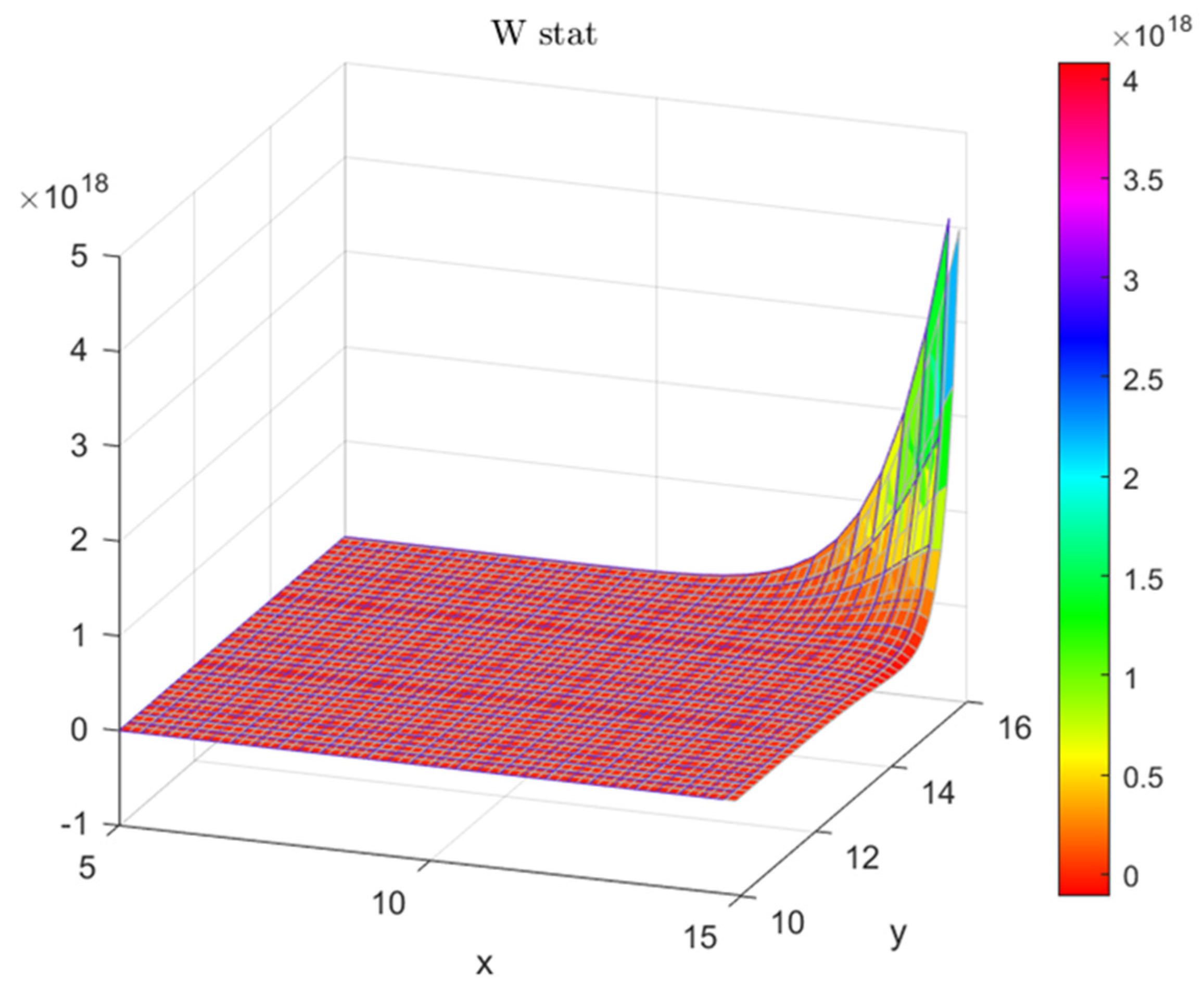
Appendix A.2. Polar Plot of the Table of Sharpe Ratios and the GRS−W Statistic

As the delta of the angle between the test and the tangency portfolio increases as the GRS-W statistic increases, implying inefficiency. The table is based on the internal area values of Table 1 for a range of return values on the outside columns and incremental variances on the top row. Mathematics 11 02198 i003
GRS~W Stat θ = (r − rf)/s
r\s1012141610121416s/r
50.1980.2760.3280.3640.40.3330.2860.255
5.50.150.23740.2970.3390.450.3750.3210.2815.5
60.1010.1980.2650.3130.50.4170.3570.3136
6.50.0530.1580.2320.2850.550.4580.3930.3446.5
70.0050.1170.1980.2570.60.50.4290.3757
7.5 0.0770.1630.228 0.5420.4640.4067.5
8 0.0370.1290.198 0.5830.50.4388
8.5 0.0940.168 0.5360.4698.5
9 0.060.137 0.5710.59
9.5 0.0250.107 0.6070.5319.5
10 0.077 0.56310
10.5 0.047 0.59410.5
Bold numbers are r: return and s: std. dev.; p-value is <0.05 for all non-bold, non-italicized cells, implying inefficient portfolios. The italicized numbers are the GRS-W values W = [ 1 + θ ^ * 2 1 + θ ^ p 2 ] 2 1 ψ 2 1 , that correspond to efficient portfolios.

Appendix A.3. Values of the GRS-W Statistic for a Range of Angles

Test Port
ANGLE 010203040455060708090
mkt tangency port cosine (xo)1.000.980.940.870.770.710.640.500.340.170.00
01.000.000
100.980.0310.000
200.940.1320.0980.000
300.870.3330.2930.1770.000
400.770.7040.6530.5050.2780.000
450.711.0000.9400.7660.5000.1740.000
500.641.4201.3471.1370.8150.4200.2100.000
600.503.0002.8792.5322.0001.3471.0000.6530.000
700.347.5497.2916.5495.4114.0173.2742.5321.1370.000
800.1732.16331.16328.28423.87318.46115.58212.7027.2912.8790.000
900.002.6,10+322.58,10+322.35,10+321.99,10+321.56,10+321.33,10+321.10,10+326.66,10+313.12,10+318.04,10+300.000
This table provides the values of the recast GRS—test statistic and is based on the angles (in italics) stretched by the portfolio under test (test port) and the globally MV efficient portfolio (mkt tangent port). Only the lower triangular matrix is relevant because the test portfolio has to lie in the feasible zone of the ellipse. Values of the statistic close to zero (in italics) imply efficiency (say 40° test port, and 45° tangency port (cosine(.) values in Bold text (0.77, 0.71), results in a GRS-test value of 0.174). The further the location of a test portfolio from the tangency portfolio the larger the distance (GRS-test values) and the lower the portfolio efficiency. The values of N and T impact the p-values as applied to the test and not the GRS-W test per se. They are also provided in Table 2 for a set of mean-variance locations. Essentially the trigonometric test has to be digitized since there would be a very large number of mean-variance combinations and locations on the X-Y plane. A digital copy can be supplied upon request.

Appendix A.4. Risk Parity: Avoiding the Problem of Error Maximization in a Mean-Variance Optimization Framework

Lee (2011), shows that for a portfolio with a variance–covariance structure Σ, risk parity is the state when the percentage contribution to total risk (PCTR) of an asset equals that of another, resulting in an even distribution of risk across all constituent asset classes. Mathematically, as reported in Agrrawal [52] for the “bivariate (Maillard, Roncalli, and Teiletche [53] also provide the general case for n > 2 assets, and Qian [54] for the n = 2 case) n = 2 asset case, where ρ12 is the correlation, σ1, σ2 and σp the standard deviations of the assets and the portfolio, and non-negative weights such that w1 + w2 =1, the problem reduces to equating PCTRi = PCTRj  i j :
σ p 2 = w 1 2 σ 1 2 + w 2 2 σ 2 2 + + 2 w 1 w 2 ρ 12 σ 1 σ 2
P C T R 1 = w 1 σ p w 1 σ p = w 1 2 σ 1 2 + w 1 w 2 ρ 12 σ 1 σ 2 σ p 2
P C T R 2 = w 2 σ p w 2 σ p = w 2 2 σ 2 2 + w 1 w 2 ρ 12 σ 1 σ 2 σ p 2
β i = σ i p σ p 2 w i β i 1 i = 1 , 2
This also implies that wi, the weight of asset i is inversely proportional to its beta βi. Choueifaty and Coignard [55], also abstract from the classic mean-variance optimized portfolios and thereafter developed risk-parity based strategies.Yu [56], in a comprehensive study on the leading methodological issues surrounding CAPM modeling identified nine major mathematical issues that affect beta estimation, of which Agrrawal [46] and Fama and French [3] link to frequency, interval and dynamic weighting constructs that ultimately affect portfolio efficiency measures. In a recent paper, de Jong and diBartolomeo [57], discuss evolving implications of optimization that deal with new alpha sources emanating from multiple performance sources and portfolio efficiency measures. Stone et al. [58] find evidence that points to a fundamental revision in the theory of the relationship between cash levels in an financial system and central bank interest rates; this paper fundamentally recasts the GRS-W statistic based on its trigonometric properties.

Appendix A.5. Risk Parity: Efficient Portfolio Zone as a Floating Hyperplane, the Tangency Portfolio and the GRS-W Statisctic Gradient -3D Efficient Frontier with Actual ETFs

Based on large scale numerical runs with actual pricing data, using a variety of multi-asset portfolios, WRDS [26], Agrrawal [52], a stable and realistic tangency portfolio placed at 8% annual return with a standard deviation of 10% per year. Utilizing that central point a mesh grid of the GRS-W test values W = [ 1 + θ ^ * 2 1 + θ ^ p 2 ] 2 1 ψ 2 1 , were spanned for μ  (5% to 15%) and σ  (5% to 25%). The gradient of the Z-axis values is indicative of the inefficiencies associated with even minor perturbations in the mean-variance space around the tangency portfolio (blue sphere). The floating hyperplane is the efficiency space projected around the tangency portfolio.
Mathematics 11 02198 i004
At a reviewer’s suggestion, a set of highly liquid and diversified Exchange traded Funds -ETFs (VT, VTI, IWM, VEU, BND, GLD, AOK, AOM, UUP, FXE, IYR), were plotted in the mean-variance-GRS-test space. As can be seen in the figure with the multiple spheres, these ETFs plotted around the bright-blue tangency portfolio. However, this efficient frontier is now an “efficient dome” and the GRS-W test is the Z-axis, making it visually quite apparent which of the assets are in the efficiency zone.
Mathematics 11 02198 i005
The author will be glad to provide additional granularity and the implementation of Matlab’s #fmesh (f) protocol to generate these analytics. It can be seen that the efficiency zone is in the vicinity of the GRS-W value of around zero, implying portfolio efficiency. These are not some randomly chosen ETFs, they represent the major asset-classes that extend beyond the equity market to the various components of the capital markets (Agrrawal [52]. One desirable attribute of these, apart from automatic diversification and high liquidity is low within pair correlation and a lower matrix covariance structure, following from Equation (3) earlier in the text. C o r r e l a t i o n = x 1 · x 2 η 1 x 1 η 1 1 x 2 η 1 1 ρ x 1 x 2 = c o v x 1 x 2 σ x 1 σ x 2 .

References

  1. Gibbons, M.R.; Ross, S.; Shanken, J. A Test of the Efficiency of the Given Portfolio. Econometrica 1989, 57, 1121–1152. [Google Scholar] [CrossRef]
  2. Galea, M.; Cademartori, D.; Curci, R.; Molina, A. Robust Inference in the Capital Asset Pricing Model Using the Multivariate t-distribution. J. Risk Financ. Manag. 2020, 13, 123. [Google Scholar] [CrossRef]
  3. Fama, E.F.; French, K.R. A five-factor asset pricing model. J. Financ. Econ. 2015, 116, 1–22. [Google Scholar]
  4. Gustafson, K. Operator Trigonometry of Multivariate Finance. J. Multivar. Anal. 2010, 101, 374–384. [Google Scholar] [CrossRef]
  5. Gustafson, K. A New Financial Risk Ratio. J. Stat. Comput. Simul. 2015, 85, 2682–2692. [Google Scholar] [CrossRef]
  6. Rodriguez, R.J. Graphical Portfolio Analysis. Financ. Rev. 1996, 31, 869–884. [Google Scholar]
  7. Roll, R. A critique of the asset pricing theory’s tests Part I: On past and potential testability of the theory. J. Financ. Econ. 1977, 4, 129–176. [Google Scholar] [CrossRef]
  8. Chen, J.M. The Capital Asset Pricing Model. Encyclopedia 2021, 1, 915–933. [Google Scholar] [CrossRef]
  9. Hu, S.; Li, D.; Jia, J.; Liu, Y. A Self-Learning Based Preference Model for Portfolio Optimization. Mathematics 2021, 9, 2621. [Google Scholar] [CrossRef]
  10. Bodnar, T.; Schmid, W. Econometrical analysis of the sample efficient frontier. Eur. J. Financ. 2009, 15, 317–335. [Google Scholar] [CrossRef]
  11. Cueto, J.M.; Grané, A.; Cascos, I. How to Explain the Cross-Section of Equity Returns through Common Principal Components. Mathematics 2021, 9, 1011. [Google Scholar] [CrossRef]
  12. Ryan, N.; Ruan, X.; Zhang, J.E.; Zhang, J.A. Choosing Factors for the Vietnamese Stock Market. J. Risk Financ. Manag. 2021, 14, 96. [Google Scholar] [CrossRef]
  13. Suárez, J.; Alonso-Conde, A.B. Relative Entropy and Minimum-Variance Pricing Kernel in Asset Pricing Model Evaluation. Entropy 2020, 22, 721. [Google Scholar] [CrossRef] [PubMed]
  14. Solórzano-Taborga, P.; Alonso-Conde, A.B.; Rojo-Suárez, J. Data Envelopment Analysis and Multifactor Asset Pricing Models. Int. J. Financ. Stud. 2020, 8, 24. [Google Scholar] [CrossRef]
  15. Barillas, F.; Kan, R.; Robotti, C.; Shanken, J. Model Comparison with Sharpe Ratios. J. Financ. Quant. Anal. 2020, 55, 1840–1874. [Google Scholar] [CrossRef]
  16. Sharpe, W.F. Mutual Fund Performance. J. Bus. 1966, 39, 119–138. Available online: http://www.jstor.org/stable/2351741 (accessed on 1 March 2023). [CrossRef]
  17. Kamstra, M.; Shi, R. A Note on the GRS Test; Technical Report; Department of Economics, University of California at Riverside: Riverside, CA, USA, 2021. [Google Scholar]
  18. Fletcher, J. An Empirical Examination of the Incremental Contribution of Stock Characteristics in UK Stock Returns. Int. J. Financ. Stud. 2017, 5, 21. [Google Scholar] [CrossRef]
  19. Vigo-Pereira, C.; Laurini, M. Portfolio Efficiency Tests with Conditioning Information—Comparing GMM and GEL Estimators. Entropy 2022, 24, 1705. [Google Scholar] [CrossRef]
  20. Basak, G.K.; Jagannathan, R.; Sun, G. A Direct Test for the Mean Variance Efficiency of a Portfolio. J. Econ. Dyn. Control 2002, 26, 1195–1215. [Google Scholar] [CrossRef]
  21. Kim, J.H.; Robinson, A.P. Interval-Based Hypothesis Testing and Its Applications to Economics and Finance. Econometrics 2019, 7, 21. [Google Scholar] [CrossRef]
  22. Shanken, J. 23 Statistical methods in tests of portfolio efficiency: A synthesis. Handb. Stat. 1996, 14, 693–711. [Google Scholar] [CrossRef]
  23. MacKinlay, A.C. Multifactor models do not explain deviations from the CAPM. J. Financ. Econ. 1995, 38, 3–28. [Google Scholar] [CrossRef]
  24. Roll, R.; Ross, S.A. On the Cross-Sectional Relation between Expected Returns and Betas. J. Financ. 1994, 49, 101. [Google Scholar] [CrossRef]
  25. Zhou, G. Asset-pricing Tests under Alternative Distributions. J. Financ. 1993, 48, 1927–1942. [Google Scholar] [CrossRef]
  26. WRDS. CRSP Pricing Data on Stocks. Wharton Research Data Services. 2023. Available online: https://wrds-www.wharton.upenn.edu/ (accessed on 1 March 2023).
  27. Agrrawal, P. An automation algorithm for harvesting capital market information from the web. Manag. Financ. 2009, 35, 427–438. [Google Scholar]
  28. Bodnar, T.; Gupta, A.K.; Vitlinskyi, V.; Zabolotskyy, T. Statistical Inference for the Beta Coefficient. Risks 2019, 7, 56. [Google Scholar] [CrossRef]
  29. Fama, E.F.; French, K.R. Common risk factors in the returns on stocks and bonds. J. Financ. Econ. 1993, 33, 3–56. [Google Scholar] [CrossRef]
  30. Hou, K.G.; Karolyi, G.A.; Kho, B. What Factors Drive Global Stock Returns? Rev. Financ. Stud. 2011, 24, 2527–2574. [Google Scholar] [CrossRef]
  31. Ehsani, S.; Linnainmaa, J.T. Factor Momentum and the Momentum Factor. J. Financ. 2022, 77, 1877–1919. [Google Scholar] [CrossRef]
  32. Merton, R.C. An analytical derivation of the efficient frontier. J. Financ. Quant. Anal. 1972, 7, 1851–1872. [Google Scholar] [CrossRef]
  33. Gómez–Déniz, E.M.E.; Ghitany, M.E.; Gupta, R.C. A bivariate generalized geometric distribution with applications. Commun. Stat. Theory Methods 2017, 46, 5453–5465. [Google Scholar] [CrossRef]
  34. Danko, J.; Soltés, V.; Bindzar, T. Portfolio creation using graph characteristics and testing its performance. Montenegrin J. Econ. 2022, 18, 7–17. [Google Scholar] [CrossRef]
  35. MacKinlay, C.A.; Richardson, M. Using Generalized Method of Moments to Test Mean-Variance Efficiency. J. Financ. 1991, 46, 511–527. [Google Scholar] [CrossRef]
  36. Black, F. Capital Market Equilibrium with Restricted Borrowing. J. Bus. 1972, 45, 444–454. [Google Scholar]
  37. Buckle, D. The Impact of Options on Investment Portfolios in the Short-Run and the Long-Run, with a Focus on Downside Protection and Call Overwriting. Mathematics 2022, 10, 1563. [Google Scholar] [CrossRef]
  38. Best, M.J. Equivalence of some Quadratic Programming Algorithms. Math. Program. 1984, 30, 71–87. [Google Scholar] [CrossRef]
  39. Best, M.J.; Grauer, R.R. On the Sensitivity of Mean-Variance-Efficient Portfolios to Changes in Asset Means: Some Analytical and Computational Results. Rev. Financ. Stud. 1991, 42, 315–342. [Google Scholar]
  40. Lee, W. Risk On/Risk Off. J. Portf. Manag. 2012, 38, 28–39. [Google Scholar]
  41. Kuhn, H.W.; Tucker, A.W. Nonlinear programming. In Proceedings of the Second Berkeley Symposium on Mathematical Statistics and Probability 1950, Berkeley, CA, USA, 31 July–12 August 1950; pp. 481–492. [Google Scholar]
  42. Greene, W.H. Econometric Analysis; Prentice Hall: Hoboken, NJ, USA, 2002; ISBN 10: 0130661899; ISBN 13: 9780130661890. [Google Scholar]
  43. Shefrin, H.M.; Statman, M. Behavioral Capital Asset Pricing Theory. J. Financ. Quant. Anal. 1994, 29, 323–349. [Google Scholar] [CrossRef]
  44. Glabadanidis, P. Another Test of the Efficiency of a Given Portfolio. SSRN Electron. J. 2015. [Google Scholar] [CrossRef]
  45. Jurdi, D.J. Predicting the Australian equity risk premium. Pac. Basin Financ. J. 2022, 71, 101683. [Google Scholar] [CrossRef]
  46. Agrrawal, P.; Gilbert, F.W.; Harkins, J. Time Dependence of CAPM Betas on the Choice of Interval Frequency and Return Timeframes: Is There an Optimum? J. Risk Financ. Manag. 2022, 15, 520. [Google Scholar] [CrossRef]
  47. Bazhutov, D.; Betzer, A.; Stehle, R. Beta estimation in the European network regulation context: What matters, what doesn’t, and what is indispensable. Financ. Mark. Portf. Manag. 2023. [Google Scholar] [CrossRef]
  48. Fama, E.F.; French, K.R. The Cross-Section of Expected Stock Returns. J. Financ. 1992, 47, 427–465. [Google Scholar] [CrossRef]
  49. Agrrawal, P. On Certain Aspects of the Ex Ante CAPM. Ph.D. Dissertation, University of Alabama, Tuscaloosa, AL, USA, 1996. [Google Scholar]
  50. Markowitz, H. Portfolio Selection. J. Financ. 1952, 7, 77–91. [Google Scholar] [CrossRef]
  51. Balbás, A.; Balbás, B.; Balbás, R. Minimizing measures of risk by saddle point conditions. J. Comput. Appl. Math. 2010, 234, 2924–2931. [Google Scholar] [CrossRef]
  52. Agrrawal, P. Using Index ETFs for Multi-Asset-Class Investing: Shifting the Efficient Frontier Up. J. Beta Investig. Strateg. 2013, 4, 83–94. [Google Scholar]
  53. Maillard, S.; Roncalli, T.; Teïletche, J. The Properties of Equally-Weighted Risk Contributions Portfolios. J. Portf. Manag. 2010, 36, 60–70. [Google Scholar] [CrossRef]
  54. Qian, E. On the Financial Interpretation of Risk Contribution: Risk Budgets Do Add Up. J. Investig. Manag. 2006, 4, 41–51. [Google Scholar] [CrossRef]
  55. Choueifaty, Y.; Coignard, Y. Toward Maximum Diversification. J. Portf. Manag. 2008, 35, 40–51. [Google Scholar] [CrossRef]
  56. Yu, Z. Cross-Section of Returns, Predictors Credibility, and Method Issues. J. Risk Financial Manag. 2023, 16, 34. [Google Scholar] [CrossRef]
  57. de Jong, M.; diBartolomeo, D. Multiple Alpha Sources and Portfolio Design. J. Asset Manag. 2021, 22, 389–390. [Google Scholar] [CrossRef]
  58. Stone, A.L.; Gup, B.E.; Lee, J. New insights about the relationship between corporate cash holdings and interest rates. J. Econ. Finan. 2018, 42, 33–65. [Google Scholar] [CrossRef]
Figure 1. The geometric basis of the GRS-W test statistic. The test coordinates of the EW portfolio (P) and the tangency portfolio (M) are plotted relative to the mean-variance efficient frontier. The further away P is from the tangency portfolio, the less efficient the portfolio P is.
Mathematics 11 02198 g001
Figure 2. Results of an actual simulation are plotted here, the MV portfolio (red square) and the test portfolio (triangular orange) are also utilized to derive the actual GRS−W statistic value (Table 2). The Rf rate is 1%.
Mathematics 11 02198 g002
Figure 3. A plot of the left panel of Table 1, showing the spike in the GRS−W as variance approaches 16% with a low return of 5%, high “W stat” values imply inefficiency of the test portfolio.
Mathematics 11 02198 g003
Table 1. Showing the values of the GRW-W test statistic and the Sharpe ratio θ.
GRS~W Stat θ = (r − rf)/s
r\s10.0012.0014.0016.0010.0012.0014.0016.00s/r
5.000.1980.2760.3280.3640.4000.3330.2860.2505.00
5.500.1500.23740.2970.3390.4500.3750.3210.2815.50
6.000.1010.1980.2650.3130.5000.4170.3570.3136.00
6.500.0530.1580.2320.2850.5500.4580.3930.3446.50
7.000.0050.1170.1980.2570.6000.5000.4290.3757.00
7.50 0.0770.1630.228 0.5420.4640.4067.50
8.00 0.0370.1290.198 0.5830.5000.4388.00
8.50 0.0940.168 0.5360.4698.50
9.00 0.0600.137 0.5710.5009.00
9.50 0.0250.107 0.6070.5319.50
10.00 0.077 0.56310.00
10.50 0.047 0.59410.50
Bold numbers are r: return and s: std. dev.; p-value is <0.05 for all non-bold, non-italicized cells, implying inefficient portfolios. The italicized numbers are the GRS-W values W = [ 1 + θ ^ * 2 1 + θ ^ p 2 ] 2 1 ψ 2 1 , that correspond to efficient portfolios.
Table 2. These represent a range of actual GRS-W test statistic values and the associated Sharpe ratio values for a set of mean-variance points (as applied in Figure 2). This table has the p-values as well. N = 30 and a 10-year weekly period of T = 520. The top panel of the table illustrates the values arrived in the first two rows of the larger table, with the first row corresponding to the tangency portfolio (7.93 r, 9.83 σ), which is also applied in Figure 2, as the tangency portfolio on the efficient frontier. Cells in bold text are the efficient portfolios with low GRS-W statistics.
Tangency Portfolio (*)Test Portfolio (p)
mean, r7.9310.50
risk free, rf1.001.00
sigma, s9.838.00
θ = (r − rf)/s0.7051.188
GRS~W Stat 0.046
NNo. of Assets30
TNo. of Weekly Intervals520
XF 0.759
p-valueRej. H0 (is an Efficient Port) iff p~00.8202
Mean, rSigma, sθ = (r − rf)/sGRS~W StatNTXFp-Value
Tangency Portfolio (*)7.939.830.705 No. of AssetsNo. of Weekly Intervals Rej. H0 (Efficient Port) iff p~0
Test Portfolio (p)10.5016.000.5940.047305200.7630.81564721900Eff.
Test Portfolio (p)3.0010.000.20.3737305206.1150.00000000000Not Efficient
Test Portfolio (p)5.0010.000.4000.198305203.2380.00000004498Not Efficient
Test Portfolio (p)5.5010.000.4500.150305202.4480.00004374410Not Efficient
6.0010.000.5000.101305201.6520.01746340000Not Efficient
6.5010.000.5500.053305200.8610.68131012700Eff.
7.0010.000.6000.005305200.0811.00000000000Eff.
Test Portfolio (p)5.0012.000.3330.276305204.5130.00000000000Not Efficient
5.5012.000.3750.237305203.8840.00000000012Not Efficient
6.0012.000.4170.198305203.2380.00000004498Not Efficient
6.5012.000.4580.158305202.5800.00001444100Not Efficient
7.0012.000.5000.117305201.9170.00279042500Not Efficient
7.5012.000.5420.077305201.2560.16816038300Eff.
8.0012.000.5830.037305200.5990.95601098600Eff.
Test Portfolio (p)5.0014.000.2860.328305205.3660.00000000000Not Efficient
5.5014.000.3210.297305204.8620.00000000000Not Efficient
6.0014.000.3570.265305204.3360.00000000000Not Efficient
6.5014.000.3930.232305203.7930.00000000028Not Efficient
7.0014.000.4290.198305203.2380.00000004498Not Efficient
7.5014.000.4640.163305202.6740.00000646460Not Efficient
8.0014.000.5000.129305202.1070.00067275200Not Efficient
8.5014.000.5360.094305201.5390.03571892400Not Efficient
9.0014.000.5710.060305200.9730.50892160100Eff.
9.5014.000.6070.025305200.4130.99780363100Eff.
Test Portfolio (p)5.0016.000.2500.364305205.9580.00000000000Not Efficient
5.5016.000.2810.339305205.5490.00000000000Not Efficient
6.0016.000.3130.313305205.1170.00000000000Not Efficient
6.5016.000.3440.285305204.6670.00000000000Not Efficient
7.0016.000.3750.257305204.2020.00000000001Not Efficient
7.5016.000.4060.228305203.7240.00000000053Not Efficient
8.0016.000.4380.198305203.2380.00000004498Not Efficient
8.5016.000.4690.168305202.7450.00000351764Not Efficient
9.0016.000.5000.137305202.2490.00022052900Not Efficient
9.5016.000.5310.107305201.7520.00899892900Not Efficient
10.0016.000.5630.077305201.2560.16816038300Eff.
10.5016.000.5940.047305200.7630.81564721900Eff.
Disclaimer/Publisher’s Note: The statements, opinions and data contained in all publications are solely those of the individual author(s) and contributor(s) and not of MDPI and/or the editor(s). MDPI and/or the editor(s) disclaim responsibility for any injury to people or property resulting from any ideas, methods, instructions or products referred to in the content.

