A New Self-Tuning Deep Neuro-Sliding Mode Control for Multi-Machine Power System Stabilizer

Abstract

In order to increase the accuracy and improve the performance of the power system stabilizer (PSS) controller compared to the methods presented in other studies, this paper presents a new method for tuning sliding mode control (SMC) parameters for a PSS using a deep neural network. This controller requires fast switching which can create unwanted signals. To solve this problem, a boundary layer is used. First, the equations of a multi-machine power system are converted into the standard form of sliding mode control, and then the sliding surfaces are determined with three unknown parameters. Calculating and determining the optimal values (at any moment) for these parameters are fundamental challenges. A deep neural network can overcome this challenge and adjust the control system regularly. In the simulation, a power system with 4 machines and 11 buses is implemented and both phase-to-ground and three-phase errors are applied. The simulation results clearly show the good performance of the proposed method and especially the importance of the deep neural network in the SMC structure compared to other methods.

1. Introduction

The stability and robustness of the voltage in a power system are essential issues and the priorities of every electric company. In recent years, various methods have been proposed to increase the dynamic stability of power systems. Modern voltage regulators and quick-response excitation systems can be used to improve transient stability in the system by increasing the car’s synchronizing torque but may adversely affect the damping of rotor oscillations. A suitable solution to this problem is to equip the generator with a controller that inserts an additional signal at the reference voltage input in the automatic voltage regulator. This device is called a power system stabilizer (PSS) [1,2,3,4,5,6]. Numerous control methodologies have been proposed for PSS design, among which classic PSSs with after-phase-pre-phase compensators have been used by most companies due to their simple structure, flexibility, and reasonable implementation. Although, the efficiency of these stabilizers is significantly reduced by changing the operating conditions of the system in normal operation. Because power systems are highly nonlinear, classical PSSs with fixed parameters cannot withstand drastic changes in system operating conditions. Additionally, changes in the automatic voltage regulating parameters cause drastic changes in the state of the system. Therefore, in practice, the classical stabilizer will not work well [7,8,9]. There are many research studies on PSS in power systems, including the optimal placement of PSSs, coordination of PSSs, and the use of more efficient methods in PSS design [10]. In the recent context, the use of optimal control theory [11], adaptive controllers [12], as well as methods such as the use of artificial neural networks [13,14,15] was presented.

Recently, with the development of artificial intelligence (AI), many studies have been conducted in the field of using them to design PSSs [16,17,18]. Although using this method has many advantages in improving system performance, it has disadvantages such as increasing the number of layers in each neuron and also increasing its training time [19,20,21]. Another method that has recently received great attention and is used to design PSSs is fuzzy logic [22,23,24,25]. In this method, with the previous knowledge of the system, researchers have proceeded to design PSSs. The fuzzy logic method has been used to design PSSs in [26,27,28]. Along with artificial intelligence, as mentioned, optimization algorithms are also being used a lot recently. In [29], simulated annealing (SA) is introduced to tuning the coefficients of PSSs. Of course, the possibility of failure of this method is also very high. In order to determine PSSs, in [10], an improved atom search optimization algorithm was proposed, which has very good performance and accuracy. Other optimization methods such as tabu search (TS) and genetic algorithm (GA) have also been mentioned in many studies [16,30,31,32].

One of the methods used in designing controllers of nonlinear systems is the sliding mode control (SMC) method. This method has been utilized to control robots, motors, and mechanical systems, and has been shown to ensure the optimal behavior of the closed-loop system [33,34]. The application of sliding mode control theory to design a power system stabilizer using the linearized model of the system has been used in [35,36]. Today, neuro-sliding mode control is used in much research and for various applications. For example, this method has been used to design and control quadrotor UAVs [37,38,39,40,41]. neuro-sliding mode controls have also shown a very good response in several studies for controlling nonlinear systems with uncertainty and have many advantages over other methods [42,43]. In addition to all these applications, with the growth of renewable systems, neuro-sliding mode controls have been recently used in renewable systems [44,45,46]. In [47,48], this method was proposed to control DFIGs. One of the disadvantages of using the linearized model of the system to design the controller is the reduction in the controller efficiency in the event of large disturbances which also cause severe changes in the system parameters. In this paper, the proposed sliding controller was designed using a nonlinear system model that was converted to a normal shape using a suitable converter. Since this controller requires a very fast switching mechanism, it produces undesirable fluctuations in the system, and the presence of these fluctuations may activate unmodulated system dynamics. A suitable method to eliminate these fluctuations employed in this paper was to use a boundary layer.

The headline innovations are:

• Introducing a new delayed deep neural network.
• Designing a sliding mode control system with six adjustable parameters (in previous works, there were usually two or three adjustable parameters).
• The development of the proposed control system for synchronizing a power system.

The contents of this article are as follows: In the second part, the dynamic model of the synchronous generator will be explained. In the third part, the design principles of sliding mode controllers will be stated. In the fourth part, to facilitate the design of the nonlinear controller for the system, using a suitable conversion, the nonlinear model of the synchronous generator will be converted to normal, and then the proposed sliding controller for the system will be introduced. In the fifth part, the stabilizer of the classical power system, which is based on post-phase-pre-phase compensators, will be introduced. Finally, in the sixth part, the results of computer simulations performed on the nonlinear system using the proposed method and the classical design method will be presented and compared.

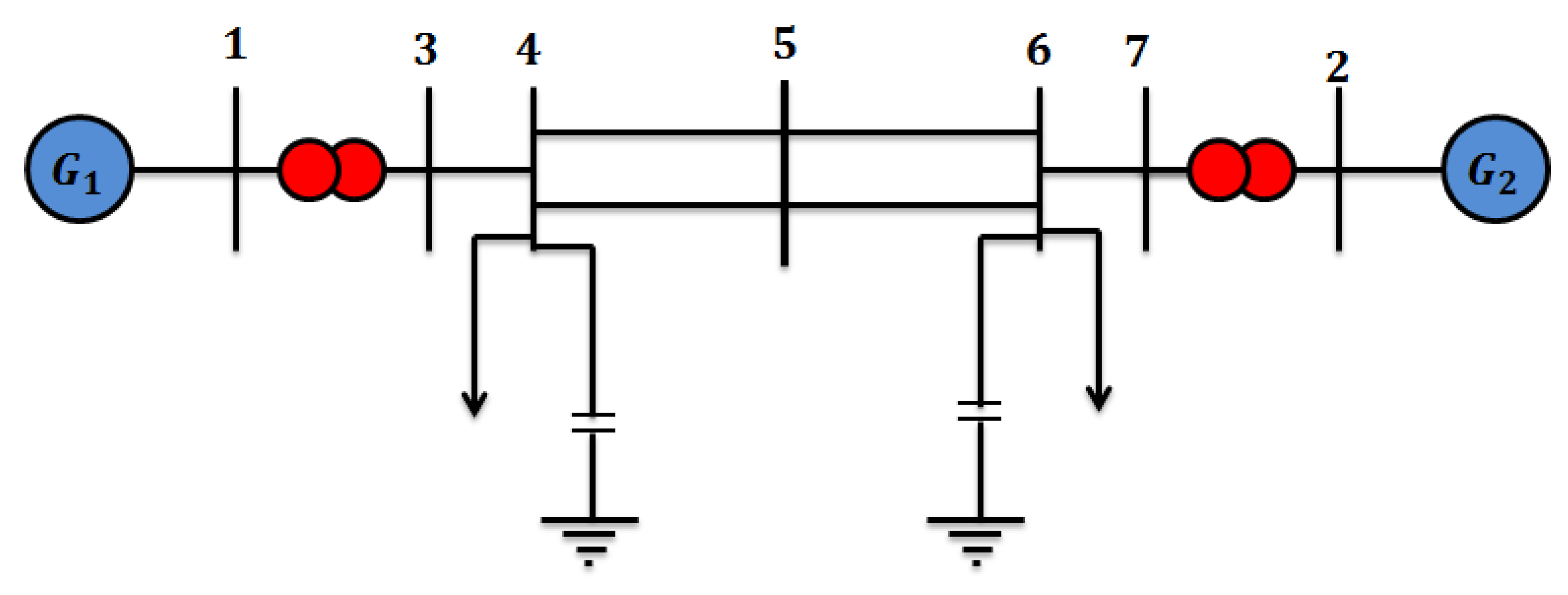
2. Dynamic Model of Synchronous Generator

A standard multi-machine power system consisting of two synchronous generators is shown in Figure 1. This system has two zones, each of which has one synchronous generator (G₁ or G₂) equipped with excitation control systems. Buses 1 and 2 are connected to generators, and buses 3 to 7 form the network topology. In the following analysis, while expressing the relationships governing the power system (generators), they will be also explained. Note that the symbols are described in

Table A1. Nomenclature.

Symbol	Definition	Symbol	Definition
$\delta \left(t\right)$	rotor angle	$\omega \left(t\right)$	rotor angular speed
$P_e\left(t\right)$	mechanical power of generator input	$x_d$	generator reactance in d direction
$x_d^{\prime }$	transient generator reactance in d direction	$X_d$	total generator reactance in d direction
$X_d^{\prime }$	system with $k_C$ gain	$T_{do}^{\prime }$	short circuit transient time
$V_s$	infinite bus voltage	${\omega }_o$	synchronous velocity of the generator
$H$	inertia constant of the generator	$K_D$	damping constant of the generator
$r\left(t\right)$	state of neurons	$b(t)$	time varying bias
$u_j\left(t\right)$	the controller input of the system	$u_{dj}$	input of the system controller
$f(a(t))$	combining the data signal $P(t)$	$r(t-{\tau }_d)$	time-delayed feedback signals modulated by the functions $M_d$
$x_{1dj}$	desired value of state ${\mathrm{x}}_{1\mathrm{j}}$

in the Appendix A. Equation (1) represents the state space equation of generators, which is expressed in three states.

$$\left\{\begin{array}{c}\frac{d}{dt}\delta \left(t\right)=\omega \left(t\right)-{\omega }_o\hfill \\ \frac{d}{dt}\omega =-\frac{K_D}{2H}\left(\omega \left(t\right)-{\omega }_o\right)+\frac{w_o}{2H}\left(P_m-P_e\left(t\right)\right)\hfill \\ \frac{d}{dt}{E}_q^{\prime }\left(t\right)=\frac{1}{T_{do}^{\prime }}\left(E_F\left(t\right)-E_q\left(t\right)\right)\hfill \end{array}\right.$$

(1)

All symbols are defined in Table A1 in the Appendix A. Equation (2) represents the state that the magnetic driving force of the q-axis of the generator is equivalent to the excitation coil of the generator are:

$$E_q\left(t\right)=\frac{X_d}{X_d^{\prime }}{E}_q^{\prime }\left(t\right)-\frac{x_d-x_d^{\prime }}{X_d^{\prime }}{V}_s\cos \left(\delta \left(t\right)\right)$$

(2)

Additionally, electric power is equal to:

$$E_F\left(t\right)=k_C{u}_F(t)$$

$$P_e\left(t\right)=\frac{V_s{E}_q\left(t\right)}{X_d}\sin \left(\delta \left(t\right)\right)$$

Note that $\delta \left(t\right)$ is the rotor angle, $\omega \left(t\right)$ is the rotor angular speed, $P_e\left(t\right)$ is the mechanical power of generator input, $x_d$ is the generator reactance in the d direction, $x_d^{\prime }$ is the transient generator reactance in the d direction, $X_d$ is the total generator reactance in the d direction, $X_d^{\prime }$ is the transient total generator reactance in the d direction, $u_F(t)$ is the amplifier input of the excitation system with $k_C$ gain, $T_{do}^{\prime }$ is the short circuit transient time, $V_s$ is the infinite bus voltage, ${\omega }_o$ is the synchronous velocity of the generator, $H$ is the inertia constant of the generator, and $K_D$ is the damping constant of the generator. The system states for the j-th generator are determined as follows:

$$x_{1j}(t)={\delta }_j(t)$$

$$x_{2j}\left(t\right)={\omega }_j\left(t\right)-{\omega }_{oj}$$

(3)

$$x_{3j}(t)=E_{qj}^{\prime }(t)$$

Therefore, the system state vector for each of the generators will be as follows:

$$x_j\left(t\right)={\left[x_{1j}\left(t\right)x_{2j}\left(t\right)x_{3j}\left(t\right)\right]}^T$$

(4)

To express the nonlinear equations of the system more clearly, the constants are defined as follows for each of the generators:

$${\alpha }_{1j}=-\frac{K_{Dj}}{2H_j}$$

$${\alpha }_{2j}=-\frac{{\omega }_{oj}}{2H_j{X}_{dj}^{\prime }}{V}_S$$

$${\alpha }_{3j}=\frac{{\omega }_{oj}\left(x_{dj}-x_{dj}^{\prime }\right)}{4H_j{X_{dj}X}_{dj}^{\prime }}{V}_S^2$$

(5)

$${\alpha }_{4j}=\frac{{\omega }_{oj}}{2H_j}{P}_{mj}$$

$${\alpha }_{5j}=-\frac{1}{T_{doj}^{\prime }}\frac{X_{dj}}{X_{dj}^{\prime }}$$

$${\alpha }_{6j}=\frac{x_{dj}-x_{dj}^{\prime }}{{T_{doj}^{\prime }X}_{dj}^{\prime }}{V}_S$$

Therefore, by placing Equation (5) in (1) and (2), the equations represent the j-th synchronous generator will be as follows:

$${\mathrm{ẋ}}_{1\mathrm{j}}\left(\mathrm{t}\right)={\mathrm{x}}_{2\mathrm{j}}\left(\mathrm{t}\right)$$

$${\mathrm{ẋ}}_{2\mathrm{j}}\left(\mathrm{t}\right)={{\alpha }_{1j}\mathrm{x}}_{2\mathrm{j}}\left(\mathrm{t}\right)+{{\alpha }_{2j}\mathrm{x}}_{3\mathrm{j}}\left(\mathrm{t}\right)\sin \left(x_{1j}\left(t\right)\right)+{{\alpha }_{3j}\sin (2\mathrm{x}}_{1\mathrm{j}}\left(\mathrm{t}\right))+{\alpha }_{4j}$$

(6)

$${\mathrm{ẋ}}_{3\mathrm{j}}\left(\mathrm{t}\right)={{\alpha }_{5j}\mathrm{x}}_{3\mathrm{j}}\left(\mathrm{t}\right)+{{\alpha }_{6j}\mathrm{c}\mathrm{o}\mathrm{s}(\mathrm{x}}_{1\mathrm{j}}\left(\mathrm{t}\right))+u_{j(t)}$$

where $u_j\left(t\right)$ is the controller input of the system and is considered as follows:

$$u_j\left(t\right)=\frac{k_{cj}}{T_{doj}^{\prime }}{u}_{Fj}\left(t\right)$$

(7)

We also show the desired values of the system states of each of the synchronous generators with the parameters $x_{1dj}$, $x_{2dj}$ and $x_{3dj}$. Therefore, the optimal state vector of the system is given by:

$$x_{Dj}={\left[x_{1dj}\hspace{1em}{x}_{2dj}\hspace{1em}{x}_{3dj}\right]}^T$$

The deviation of the power angle from its desired value is also considered as the controlled output of each of the generators, so:

$$y_j\left(t\right)=x_{1j}\left(t\right)-x_{1dj}$$

(8)

Additionally, using Equations (6), the values of $x_{1dj}$, $x_{2dj}$ and $x_{3dj}$ must be true in the following equations:

$$\left\{\begin{array}{c}\left(-\frac{{\alpha }_{1j}{\alpha }_{6j}}{{2\alpha }_{5j}}+{\alpha }_{3j}\right)\sin \left(2x_{1dj}\right)-\frac{{\alpha }_{2j}}{{\alpha }_{5j}}{u}_{dj}\sin \left(x_{1dj}\right)+{\alpha }_{4j}=0\hfill \\ x_{2dj}=0\hfill \\ x_{3dj}=-\frac{{\alpha }_{6j}}{{\alpha }_{5j}}\cos \left(x_{1dj}\right)-\frac{1}{{\alpha }_{5j}}{u}_{dj}\hfill \end{array}\right.$$

(9)

The $u_{dj}$ is the input of the system controller so that the system states achieve the desired values.

3. Sliding Mode Control

One of the methods used in the design of controllers of nonlinear systems is the sliding mode control method. This method is defined based on system state variables. This technique is commonly used in systems that do not have accurate knowledge of their characteristics or the system may be affected by unforeseen variables. The main advantage of this method is to make the system resistant to change. Sliding state control has shown that it can achieve the desired performance despite the uncertainty in the system parameters as well as the existence of sources of external disturbance. In this method, by using the infinitely fast switching of a part of the control signal, a stable resistive controller can be designed. On the other hand, switching causes undesirable fluctuations in the system, the existence of which may cause the activation of unmodulated system dynamics. A suitable method to eliminate these fluctuations is to use a boundary layer [49,50].

The proposed sliding mode controller is based on a three-step algorithm. The first step is to transform the original nonlinear system into a normal one. The second step is to design a linear sliding surface for the system, and the third step is to design a control signal so that it first moves the state path from the initial state to the sliding surface, and secondly, when it reaches this level, the state path remains on that surface. To describe this method, we consider the following nonlinear system of order n multi-input multi-output (MIMO):

$$\left\{\begin{array}{c}\mathrm{ẋ}=f\left(x\right)+G\left(x\right)u\hfill \\ y=h\left(x\right)\hfill \end{array}\right.$$

(10)

where x ∈$R^{n\times 1}$, u ∈$R^{m\times 1}$, and y ∈$R^{m\times 1}$ are the state vector, the input vector, and the output vector of the system, respectively, and also $f\left(x\right)\in R^{n\times 1}$, $G\left(x\right)\in R^{m\times \mathrm{m}}$ and $h\left(x\right)\in R^{m\times 1}$ are smooth vector fields. In the following the three stages, the algorithm of sliding mode controller design will be described.

3.1. Converting the System to Normal Form

Converting the given system to normal is the first step in the design process of the proposed sliding mode controller, to do this using a suitable conversion such as $\left(t\right)=T\left(x\right)$. The nonlinear system (10) is normalized as follows:

$$\left\{\begin{array}{c}\begin{array}{c}{\mathrm{ż}}_1\left(t\right)=z_2(t)\\ {\mathrm{ż}}_2\left(t\right)=z_3(t)\\ \begin{array}{c}⋮\\ {\mathrm{ż}}_{n-1}\left(t\right)=z_n\left(t\right)\end{array}\end{array}\\ {\mathrm{ż}}_n\left(t\right)=f\left(z\right)+G\left(z\right)u\end{array}،y\left(t\right)=z_1(t)\right.$$

(11)

3.2. Designing Sliding Surfaces:

In the second step, to design a sliding mode controller, a surface called sliding surface is defined. The sliding surface is the surface on which the state variables are placed to bring themselves to a steady state. Therefore, with any initial condition, the system state variables must first reach this level and then bring them to the source by referencing this level after the oscillations. The equation of each sliding level is selected in such a way that its degree is one degree less than the order of the system. A common form for determining sliding levels is as follows:

$$S_i\left(x\right)={\sum }_{k=0}^{n-1}{\rho }_{ik}{y}_i^{\left(k\right)}\left(t\right)=0\hspace{1em}\hspace{1em}\forall i=\overline{1،m}$$

(12)

In this equation, $n$ is the system order and ${\rho }_{ik}$ are tunable coefficients for obtaining desired transient response for the system outputs. m is the number of sliding surfaces.

3.3. Design of Control Functions

Control functions are selected in such a way that, firstly, from each initial state, each state x reaches the sliding surface in a limited time, and secondly, after reaching this level, the state path remains on that surface. In the sliding state control method, each of the components of the control function, $u_i$, which has a switching mechanism, are very fast and have a nonlinear structure as follows:

$$u_i=\left\{\begin{array}{c}{u}_i^{+}\left(t،x\right)\hspace{1em}{S}_i\left(x\right)>0\hfill \\ u_i^{-}\left(t،x\right)\hspace{1em}{S}_i\left(x\right)<0\hfill \end{array}\hspace{1em}\hspace{1em}\hspace{1em}\forall i=\overline{1،m}\right.$$

(13)

These control functions must be selected in such a way as to satisfy the condition of sliding control. A very common form of this condition is as follows:

$$S_i\left(x\right){\mathrm{Ṡ}}_i\left(x\right)<0\hspace{1em}\hspace{1em}\hspace{1em}\forall i=\overline{1،m}$$

(14)

4. Sliding Controller Design

The purpose of this section is to introduce a design of a controller based on the sliding control theory for the synchronous generator. Consequently, it adjusts the state of the system to its desired values and maintains the stability of the network at the point of operation in the presence of uncertainties. Equations (6) and (8), which represent the synchronous generator system, are strictly nonlinear. Thus, in the first step, to facilitate the design of the nonlinear controller, a suitable variable change $x_j\left(t\right)=z_j\left(t\right)$ is used to convert the system to normal. This variable change for each of the generators is as follows:

$$\left\{\begin{array}{c}{z}_{1j}\left(t\right)=x_{1j}\left(t\right)-x_{1dj}\hfill \\ z_{2j}\left(t\right)=x_{2j}\left(t\right)\hfill \\ z_{3j}\left(t\right)={\alpha }_{1j}{x}_{2j}\left(t\right)+{\alpha }_{2j}{x}_{3j}\left(t\right)\sin \left(x_{1j}\left(t\right)\right)+{\alpha }_{3j}\sin \left(2x_{1j}\left(t\right)\right)+{\alpha }_{4j}\hfill \end{array}\right.$$

(15)

Using Equations (9) and (15), it can be proved that if $z_j\left(t\right)$ converges to zero at $t\to \infty$, then $x_j\left(t\right)$ converges to $x_{dj}$ at $t\to \infty$. If $\sin \left(x_{1j}\left(t\right)\right)\ne 0$, the inverse of (15) is as follows:

$$\left\{\begin{array}{c}\hspace{1em}{x}_{1j}\left(t\right)=z_{1j}\left(t\right)+x_{1dj}\hfill \\ \hspace{1em}{x}_{2j}\left(t\right)=z_{2j}\left(t\right)\hfill \\ x_{3j}\left(t\right)=1∕({\alpha }_{2j}\sin \left(z_{ij}\left(t\right)+x_{idj}\right))(z_{3j}\left(t\right)-{\alpha }_{ij}{z}_{2j}\left(t\right)-{\alpha }_{3j}\sin \left(2(z_{1j}\left(t\right)+x_{idj}\right))-{\alpha }_{4j})\hfill \end{array}\right.$$

(16)

The condition of $\sin \left(x_{1j}\left(t\right)\right)\ne 0$ means that:

$$x_{1j}\left(t\right)={\delta }_j\left(t\right)\ne n\pi \hspace{1em}n=0.\pm 1.\pm 2.\dots$$

(17)

Since the operating area of the power angle of the synchronous generator is in the range (0, $\pi$), the condition $\sin \left(x_{1j}\left(t\right)\right)\ne 0$ is always in the operating area. It should be noted, however, that if ${\delta }_j\left(t\right)$ is not in the range (0, π), synchronism is lost. By placing Equation (6) in (15), the equations of the synchronous generator are obtained as follows:

$$\left\{\begin{array}{c}{\mathrm{ż}}_{1j}\left(t\right)=z_{2j}\left(t\right)\hfill \\ {\mathrm{ż}}_{2j}\left(t\right)=z_{3j}\left(t\right)\hfill \\ {\mathrm{ż}}_{3j}\left(t\right)=f_j\left(z\right)+G_j\left(z\right)u_j\hfill \end{array}\right.$$

(18)

$$y_j\left(t\right)=z_{1j}\left(t\right)$$

where:

$$\begin{gathered} f_j\left(z\right)=\left(\begin{array}{c}\left({\alpha }_{1j}+{\alpha }_{5j}\right)z_{3j}-{\alpha }_{1j}{\alpha }_{5j}{z}_{2j}\\ +\left(\frac{1}{2}{\alpha }_{ij}{\alpha }_{6j}-{\alpha }_{3j}{\alpha }_{5j}\right)\mathrm{s}\mathrm{i}\mathrm{n}(2\left(z_{ij}+x_{1dj}\right))\end{array}\right)+2{\alpha }_{3j}{z}_{2j}\cos \left(2\left(z_{ij}+x_{1dj}\right)\right) \\ +z_{2j}\mathrm{co}t\left(z_{ij}+x_{1dj}\right)\left(\begin{array}{c}{z}_{3j}-{\alpha }_{1j}{z}_{2j}\\ +{\alpha }_{3j}\sin \left(2\left(z_{ij}+x_{1dj}\right)\right)-{\alpha }_{4j}\end{array}\right)-{\alpha }_{4j}{\alpha }_{5j} \end{gathered}$$

(19)

$$G_j\left(z\right)={\alpha }_{2j}\sin \left(z_{1j}+x_{1dj}\right)$$

(20)

It should also be noted that in the main system, the functions $f_j\left(z\right)=f_{1j}\left(x\right)$ and $G_j\left(z\right)=G_{1j}\left(x\right)$ are as follows:

$$\begin{array}{c}{f}_j\left(x\right)={\alpha }_{1j}\left({\alpha }_{1j}{x}_{2j}+{\alpha }_{2j}{x}_{3j}\sin (x_{1j})+{\alpha }_{3j}\sin \left(2x_{1j}\right)+{\alpha }_{4j}\right)\hfill \\ +{\alpha }_{2j}({\alpha }_{5j}{x}_{3j}+{\alpha }_{6j}\cos \left(x_{1j}\right))sin(x_{1j})+{\alpha }_{2j}{x}_{2j}{x}_{3j}\cos \left(x_{1j}\right)+2{\alpha }_{3j}{x}_{2j}cos\left(2x_{1j}\right)\hfill \end{array}$$

(21)

and

$$G_{1j}\left(x\right)={\alpha }_{2j}\sin \left(x_{1j}\right)$$

(22)

The model obtained for the synchronous generator described in Equation (18) is used to design a sliding controller. The designed controller is then returned to the main device using the conversion $z^{-1}=T_j{x}_j$ given in Equation (16). The second step in designing a sliding controller is to determine the sliding surface. Using Equation (12), the sliding surface for the desired system is obtained as follows:

$$S_j={\ddot{y}}_j+{\rho }_{1j}{\mathrm{ẏ}}_j+{\rho }_{2j}{y}_j=z_{3j}+{\rho }_{1j}{z}_{2j}+{\rho }_{2j}{z}_{1j}$$

(23)

The constants ${\rho }_{1j}$ and ${\rho }_{2j}$ are positive scalar numbers and are selected in such a way that the desired transient response is obtained for the system output. Using Equation (15), the sliding surface equation in terms of the variables $x_{1j}$, $x_{2j}$ and $x_{3j}$ is obtained as follows:

$$S_j={\alpha }_{1j}{x_{2j}+{\alpha }_{2j}{x_{3j}\mathrm{s}\mathrm{i}\mathrm{n}(x}_{1j})+\alpha }_{3j}sin\left({2x}_{1j}\right)+{\alpha }_{4j}+{\rho }_{1j}{x}_{2j}+{\rho }_{2j}(x_{1j}-x_{1dj})$$

(24)

It should be noted that by determining the sliding level as above, the output convergence of the system output to zero is guaranteed when t → ∞ on the sliding plane $S_j\left(x\right)=0$. The third step in designing the proposed sliding mode controller is to select a control function for the system, which is as follows:

$$u_j(\mathrm{t})=\frac{-1}{G_j\left(z\right)}(f_j\left(z\right)+{\rho }_{1j}{z}_{3j}+{\rho }_{2j}{z}_{2j}+{\eta }_{j}sign\left(z_{3j}+{\rho }_{1j}{z}_{2j}+{\rho }_{2j}{z}_{1j}\right))$$

(25)

where ${\eta }_j$ is a positive scalar number and its value is determined by the designer. To investigate the condition of sliding state control by deriving Equation (23) and using Equation (18), we have:

$${\mathrm{Ṡ}}_j={\stackrel{⃛}{y}}_j+{\rho }_{1j}{ӱ}_j+{\rho }_{2j}{\mathrm{ẏ}}_j=f_j(z)+G_j({z)u}_j+{\rho }_{1j}{z}_{3j}+{\rho }_{2j}{z}_{2j}$$

(26)

By placing Equation (25) in (26), we will have:

$$\begin{array}{cc}\hfill {\mathrm{Ṡ}}_j=f_j\left(z\right)+{\rho }_{1j}{z}_{3j}& +{\rho }_{2j}{z}_{2j}\hfill \\ & +\left(-f_j\left(z\right)-{\rho }_{1j}{z}_{3j}-{\rho }_{2j}{z}_{2j}-{\eta }_{j}sign\left(z_{3j}+{\rho }_{1j}{z}_{2j}+{\rho }_{2j}{z}_{1j}\right)\right)\hfill \\ & =-{\eta }_{j}sign\left(z_{3j}+{\rho }_{1j}{z}_{2j}+{\rho }_{2j}{z}_{1j}\right)\hfill \\ & =-{\eta }_{j}sign\left(S_j\right)\hfill \end{array}$$

(27)

Thus,

$$S_j{\mathrm{Ṡ}}_j=-S_j{\eta }_{j}sign\left(S_j\right)=-{\eta }_j\left|S_j\right|<0$$

(28)

As a result, by selecting the control function in the form (25), the condition of sliding mode control for the system is met. Since ${\eta }_j$ is a strictly positive value, each state of the system, with any initial conditions, reaches a sliding surface in a limited time and moves to the origin. Since the sliding plane $S$ converges to zero at a finite time, the output $y_j\left(t\right)=z_{1j}(t)$ is also controlled based on ${\ddot{y}}_j+{\rho }_{1j}{\mathrm{ẏ}}_j+{\rho }_{2j}{y}_j=0$. Since $z_{1j}(t)$ converges to zero at t → ∞, then $z_{2j}(t)$ and $z_{3j}(t)$ also tend to zero at t → ∞.

Using Equation (16), the control function given in Equation (25) in the main device is obtained as follows:

$$\begin{gathered} u_j=\frac{1}{{\alpha }_{2j}\sin \left(x_{1j}\right)}(-({\alpha }_{1j}+{\rho }_{1j})\left(\begin{array}{c}{\alpha }_{1j}{x}_{2j}+{\alpha }_{2j}{x}_{3j}\mathrm{s}\mathrm{i}\mathrm{n}(x_{1j})\hfill \\ +{\alpha }_{3j}\sin \left({2x}_{1j}\right)+{\alpha }_{4j}\hfill \end{array}\right) \\ \hspace{1em}\hspace{1em}+\frac{1}{{\alpha }_{2j}\sin \left(x_{1j}\right)}\left(\begin{array}{c}{-\alpha }_{2j}({\alpha }_{5j}{x}_{3j}+{\alpha }_{6j}\mathrm{c}\mathrm{o}\mathrm{s}\left(x_{1j}\right)\sin (x_{1j})\hfill \\ {-\alpha }_{2j}{x}_{2j}{x}_{3j}\cos \left(x_{1j}\right)-{2\alpha }_{3j}{x}_{2j}\mathrm{c}\mathrm{o}\mathrm{s}(2x_{1j})\hfill \end{array}\right) \\ \hspace{1em}\hspace{1em}\hspace{1em}\hspace{1em}\hspace{1em}\hspace{1em}\hspace{1em}\hspace{1em}\hspace{1em}\hspace{1em}+\frac{1}{{\alpha }_{2j}\sin \left(x_{1j}\right)}\left(-{\rho }_{2j}{x}_{2j}-{\eta }_{j}sign\left(S_j\right)\right) \end{gathered}$$

(29)

where:

$$S_j={\alpha }_{1j}{x_{2j}+{\alpha }_{2j}{x_{3j}\mathrm{s}\mathrm{i}\mathrm{n}(x}_{1j})+\alpha }_{3j}sin\left({2x}_{1j}\right)+{\alpha }_{4j}+{\rho }_{1j}{x}_{2j}+{\rho }_{2j}(x_{1j}-x_{1dj})$$

(30)

Therefore, by applying the controller designed in Equations (29) and (30) and applying it to the system given in Equations (6) and (8), asymptotic convergence of $x_{1j}(t)$, $x_{2j}(t)$ and $x_{3j}(t)$ to their desired values in t → ∞ is also guaranteed.

The design of the control function of the system by utilizing the signal function causes undesirable fluctuations in the system. The presence of these fluctuations may activate the unmodulated dynamics of the system. A suitable method to eliminate these fluctuations is to use a boundary layer with width ${\epsilon }_j$ at $S_j\left(x\right)=0$. In this case, we will have:

$$\begin{gathered} u_j=\frac{1}{{\alpha }_{2j}\sin \left(x_{1j}\right)}\{(-({\alpha }_{1j}+{\rho }_{1j})\left(\begin{array}{c}{\alpha }_{1j}{x}_{2j}+{\alpha }_{2j}{x}_{3j}\mathrm{s}\mathrm{i}\mathrm{n}(x_{1j})\hfill \\ +{\alpha }_{3j}\sin \left({2x}_{1j}\right)+{\alpha }_{4j}\hfill \end{array}\right) \\ +\left(\begin{array}{c}{-\alpha }_{2j}({\alpha }_{5j}{x}_{3j}+{\alpha }_{6j}\mathrm{c}\mathrm{o}\mathrm{s}\left(x_{1j}\right)\sin (x_{1j})\\ {-\alpha }_{2j}{x}_{2j}{x}_{3j}\cos \left(x_{1j}\right)-{2\alpha }_{3j}{x}_{2j}\mathrm{c}\mathrm{o}\mathrm{s}(2x_{1j})\end{array}\right)+(-{\rho }_{2j}{x}_{2j}-{\eta }_{j}sat\left(\frac{S_j}{{\epsilon }_j}\right))\} \end{gathered}$$

(31)

where ${\epsilon }_j>0$ determines the width of the boundary layer in the vicinity of the sliding surfaces.

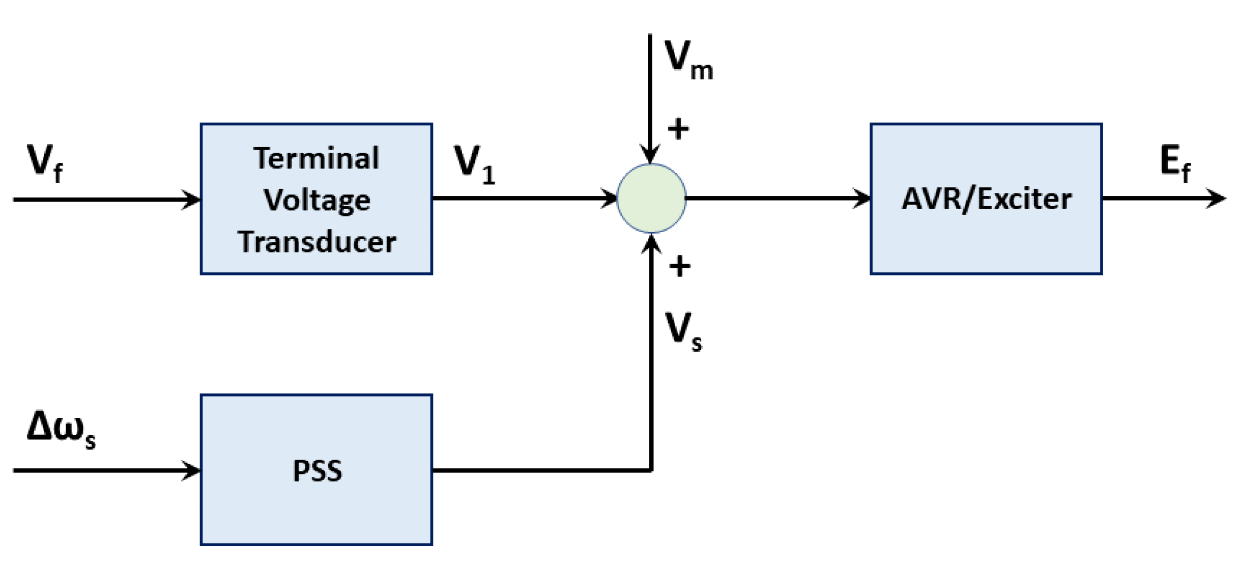
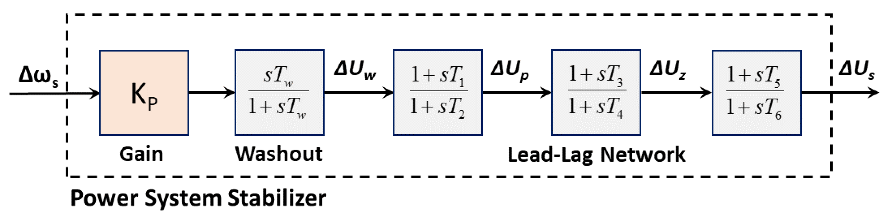
5. Comparison of Proposed and Classical Power System Stabilizer

To show the superior performance of the proposed controller, the results of using this controller are compared with the classical controller, which includes an automatic voltage regulator and power system stabilizer (AVR + PSS). In the classical method, a phase-to-phase compensator is used to dampen the electromechanical oscillations of the generator. The transfer function that is commonly used for this type of PSS is as follows:

$$G_{PSS}\left(s\right)=K_{PSS}\frac{(1+{sT}_1)}{(1+{sT}_2)}\frac{(1+{sT}_3)}{(1+{sT}_4)}\frac{{sT}_w}{(1+{sT}_w)}$$

(32)

The block diagram of this controller is shown in Figure 2.

This controller includes an IEEE standard ST1A thyristor excitation system with an automatic voltage regulator (AVR) and power system stabilizer (PSS). The power stabilization block diagram of the power system is shown in Figure 3, the various parts of which are the gain block, which has a significant effect on the damping of the rotor oscillations, and the amount of damping created by the blocking state. It acts as a high-pass filter and a compensating block, which pre-characterizes the after-phase compensation between the exciter input (PSS output) and the electric torque of the generator and provides the right phase. The time constants $T_1$, $T_2$, $T_3$ and $T_4$ must be adjusted so that an acceptable attenuation is obtained in the frequency oscillations.

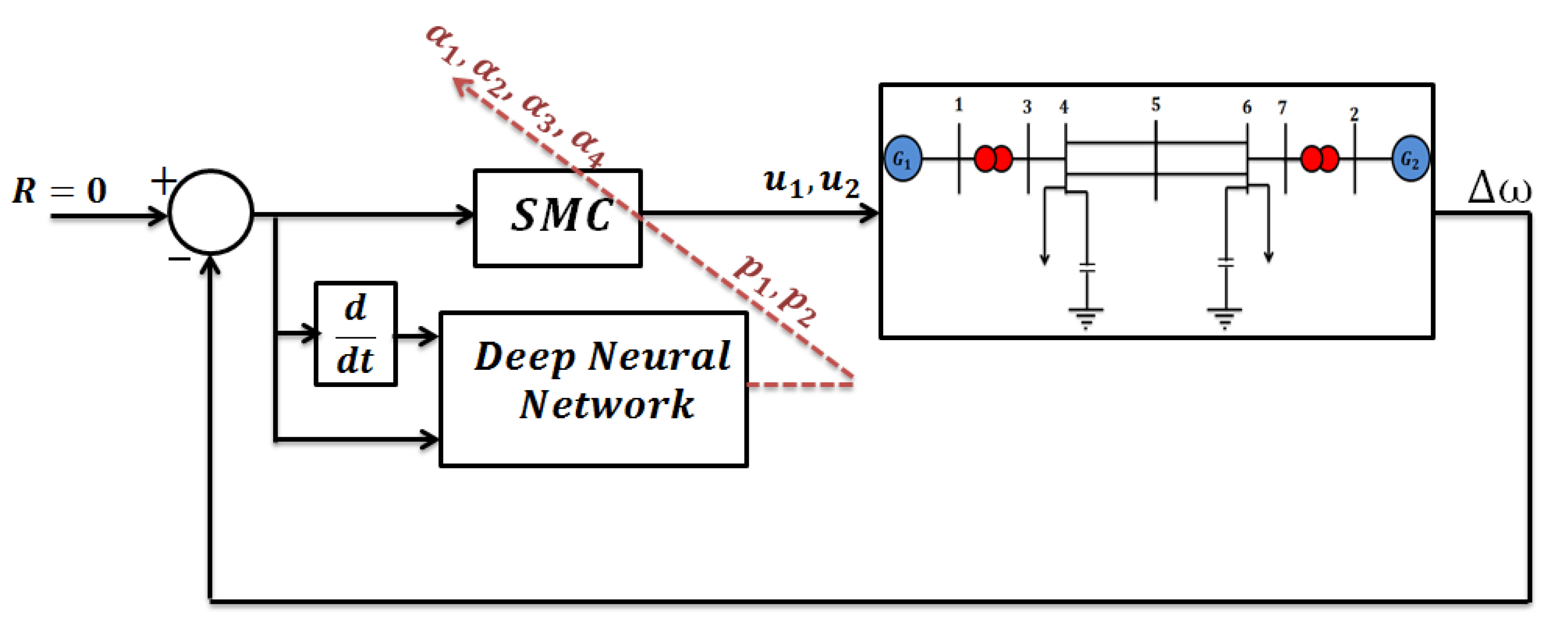
Calculation of SMS Parameters with DNN

The first step in designing phase compensation is to calculate the frequency response between the exciter input and the generator electrical torque. The frequency response desired by each machine is sensitive to the impedance of the circuit equivalent to the tonnage of its terminals but is almost independent of the dynamics of other machines. Therefore, it can be assumed that all other machines operate as infinite busbars, thus eliminating their dynamics from the response calculation. While the correct tonnage impedance is maintained at the terminals of the machine under study. Thus, the resulting phase characteristic has an almost simple shape free from the effect of the natural frequencies of external machines. The terminal voltage converter transfer function and AVR/Exciter are as follows [51,52,53]:

$$G_{TVT}\left(s\right)=\frac{1}{1+{sT}_R}$$

(33)

$$G_{AVR}\left(s\right)=K_A$$

(34)

Therefore, the AVR + PSS control equation can be written as follows:

$$E_F=K_A\left(V_{ref}-V_1+V_{supp}\right)$$

(35)

where $V_1$ is the output of the terminal voltage converter, $V_{supp}$ is the output of the power system stabilizer, and $V_{ref}$ is the reference voltage of the system. Figure 4 displays a DNN structure that can be used here. The basis of this structure is comprised of single neurons its nature need not be determined. The state of this system in continuous time mode can be calculated from Equation (36) [54,55,56].

$$\dot{r}\left(t\right)=-\propto r\left(t\right)+f(a(t))$$

(36)

where $r\left(t\right)$ given by (37).

$$r\left(t\right)=p\left(t\right)+b\left(t\right)+{\sum }_{d=1}^D{M}_d\left(t\right)r(t-{\tau }_d)$$

(37)

$r\left(t\right)$: the state of neurons.

$f(a(t))$: combining the data signal $P(t)$.

$b(t)$: time-varying bias.

$r(t-{\tau }_d)$: time-delayed feedback signals modulated by the functions $M_d$.

Methods that utilize only neural networks to fault the location must process large amounts of data, which results in slowing down the system. This method is different from other methods because in the impedance-based method is initially employed, a much smaller number of data are processed by the neural network implying a high speed of operation. Additionally, this method has a very high percentage of accuracy. Applying this method, besides precisely specifying the distance to the fault location, the line where the fault happened is also specified. As can be seen from Figure 4, the task of the deep neural network is to calculate the SMC parameters online so that the system error becomes less and less.

As seen in Figure 4, the output of the neural network is six unknown parameters of SMC. With the aim of minimizing the speed difference of the generators (synchronization), the neural network is adjusted.

It can be seen carefully in Equation (31) that six unknown parameters must be calculated at every moment to generate the control signal. These six parameters are ${\mathrm{a}}_1,\dots ,{\mathrm{a}}_2,{\mathrm{p}}_1,{\mathrm{p}}_2$. In other words, the output of the neural network is these six parameters and its input is $∆\mathsf{\omega }$ and $∆\dot{\mathsf{\omega }}$. The weights of the neural network are adjusted so that the following cost function is minimized.

$${\mathrm{J}}_{\mathrm{k}}=\frac{1}{\mathrm{N}}{\sum }_{\mathrm{k}=1}^{\mathrm{N}}{\left|∆\mathsf{\omega }\right|}_{\mathrm{k}}^2$$

(38)

where N is the length of the neural network search window and k represents each iteration. Therefore, the neural network calculates all six SMC parameters while adjusting its weights with the objective of minimizing the cost function (which is to minimize $∆\mathsf{\omega }$ here).

As can be seen in the Figure 5, increasing the number of delays leads to increasing the number of delays (feedbacks) and the dynamics of the system can be extracted better.

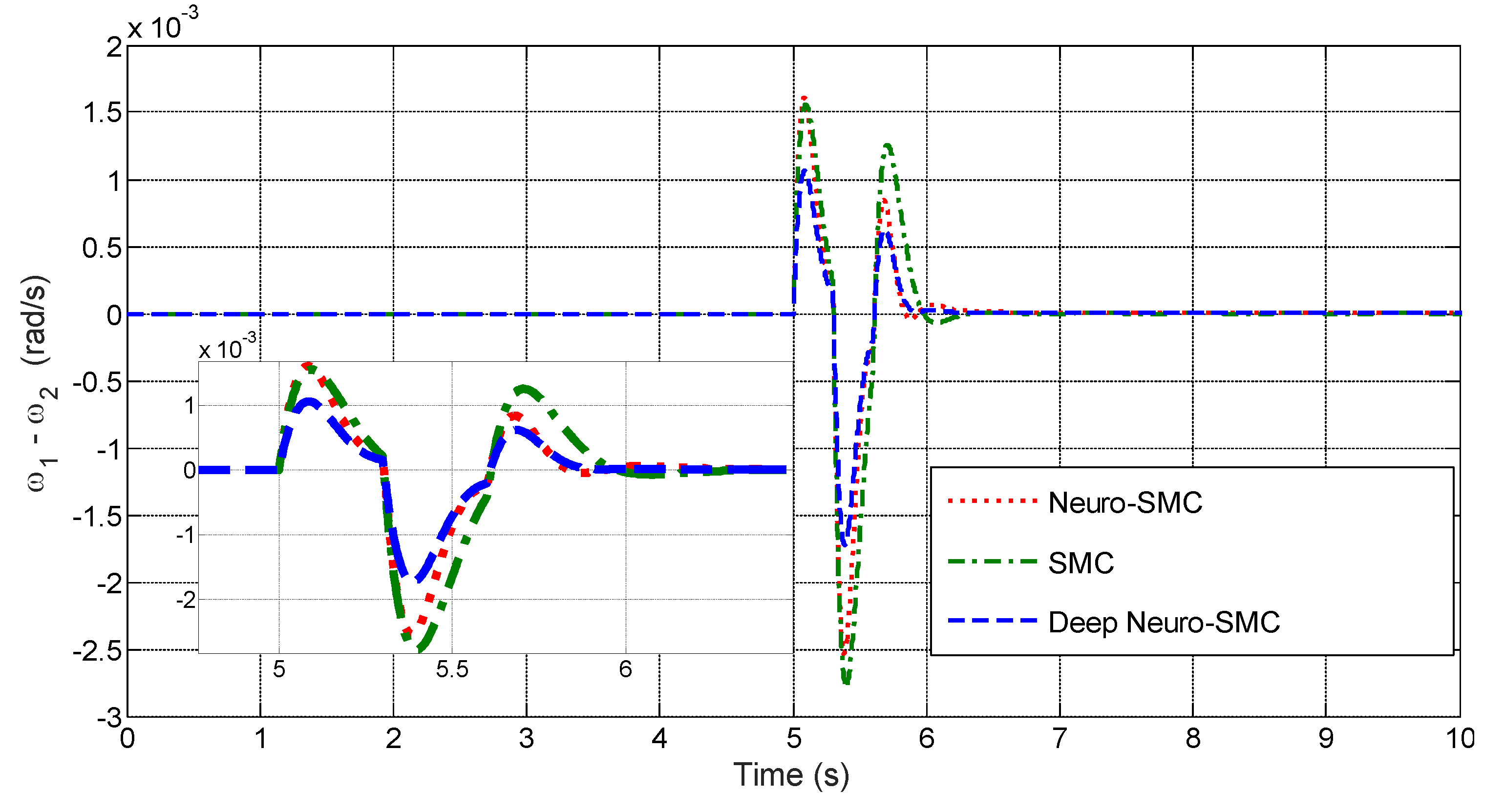
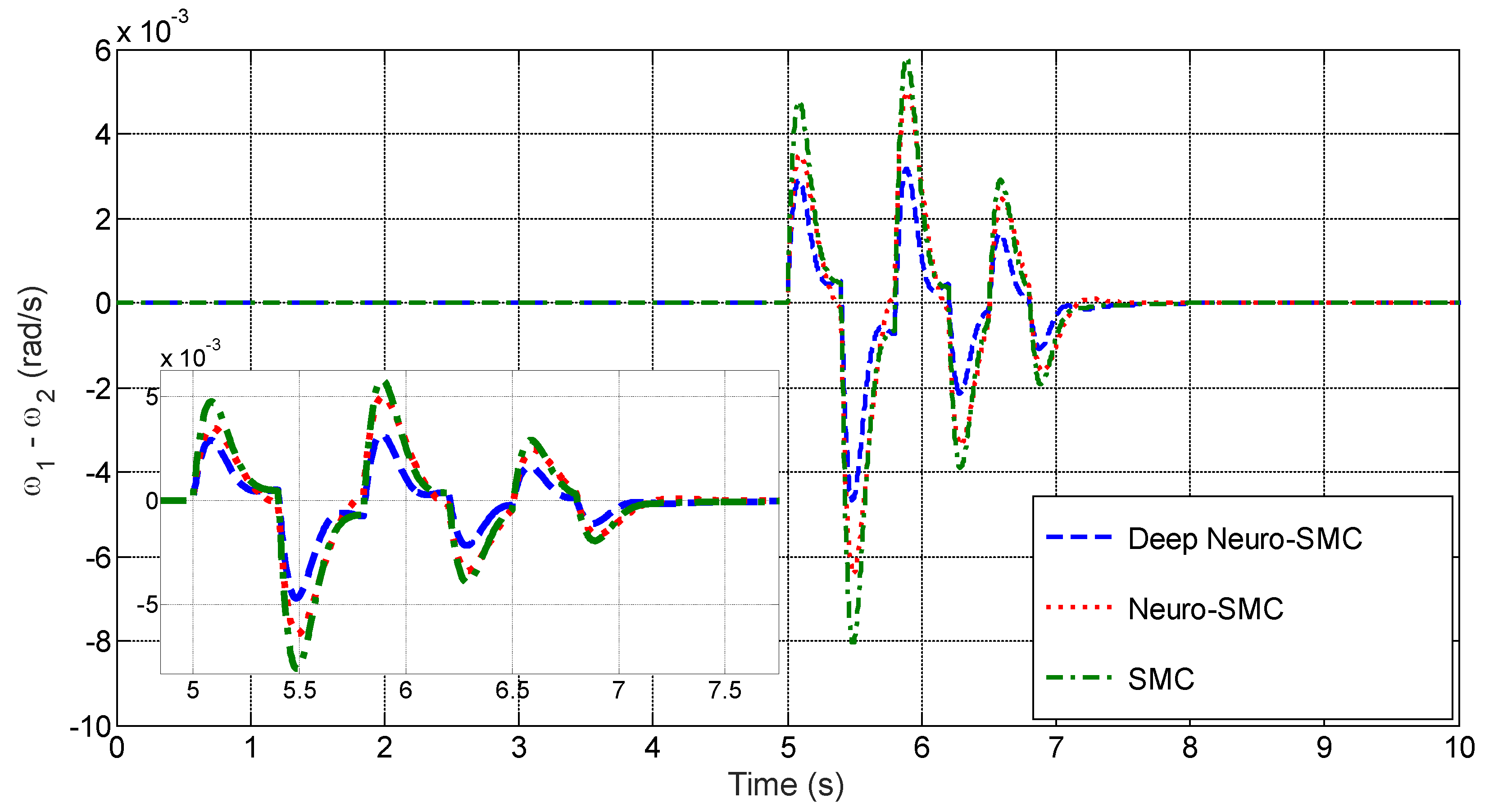
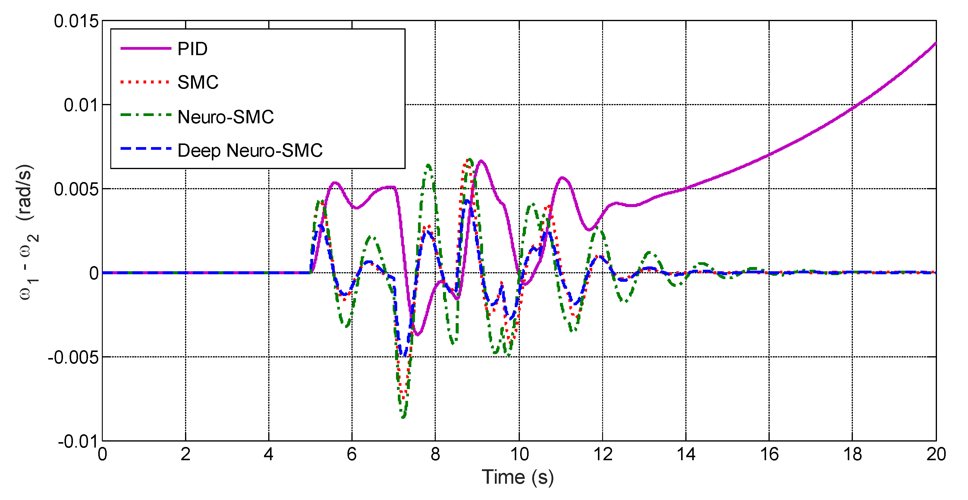
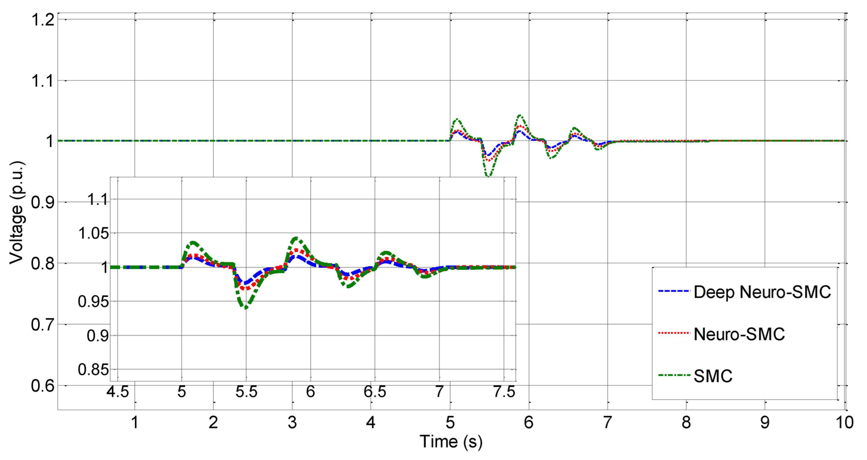
6. Simulation Results

The simulations performed in this paper were performed on the multi-machine power system shown in Figure 1. The system transmitted 400MW of energy from zone one to zone two through two transmission lines. The nominal parameters of the generators of the system under study are given in

Table A2. Nominal parameters of synchronous generators of a two-zone system.

Gen	${\mathit{R}}_{\mathit{s}}$ p.u.	${\mathit{X}}_{\mathit{d}}$ p.u.	${{\mathit{X}}^{\prime }}_{\mathit{d}}$ p.u.	${\mathit{X}}_{\mathit{q}}$ p.u.	${{\mathit{X}}^{\prime }}_{\mathit{q}}$ p.u.	${\mathit{X}}_1$ p.u.
1	0.0025	1.8	0.3	1.7	0.55	0.2
2	0.0025	1.8	0.3	1.7	0.55	0.2
3	0.0025	1.8	0.3	1.7	0.55	0.2
4	0.0025	1.8	0.3	1.7	0.55	0.2

and

Table A3. Nominal parameters of synchronous generators of two-zone system.

Gen	${{\mathit{T}}^{\prime }}_{\mathit{d}\mathit{o}}$ s	${{\mathit{T}}^{\prime }}_{\mathit{q}\mathit{o}}$ s	H s	${\mathit{K}}_{\mathit{D}}$ s	${\mathit{K}}_{\mathit{A}}$ s	${\mathit{T}}_{\mathit{R}}$ s
1	8	0.4	6.5	0	-	0.02
2	8	0.4	6.5	0	200	0.02
3	8	0.4	6.175	0	200	0.02
4	8	0.4	6.175	0	200	0.02

in the Appendix A. To evaluate the proposed algorithm for the proposed sliding model control power system stabilizer (SMCPSS) and compare it with the classical controller (AVR + PSS) and without stabilizer (NOPSS), we simulated the system under different operating conditions. It should be noted that the nonlinear model of the system was used in all the simulations performed. To read more about the theoretical relations of this discussion, you can refer to references [37,57].

Creating a Symmetric Three-Phase Error

In the first case, the system response to generating a symmetric three-phase error at $\mathrm{t}=5\mathrm{s}$ in bus number 4 is examined. Here, it is assumed that the protection relays act on time (about 0.1 s) and disconnect the damaged line from the circuit. Figure 5 shows the results of a classical SMC, a neural-network-based SMC, and a deep-neural-network-based SMC for damping fluctuations in generator rotor speeds. As can be seen in Figure 6, the deep-neural-network-based SMC has the best performance, and the neural-network-based SMC’s performance was better than the traditional SMC. One of the basic challenges of a power system is increasing the load in it. In the following, the performance of the control systems in the face of a short circuit fault and despite the load increase (up to 25% of the nominal load) is measured.

Furthermore, it can be seen from Figure 7 that despite the increase in load, the performance of the proposed control system was suitable. Although many times it caused the synchronization of two generators to take some time, the proposed method showed its effectiveness with high accuracy. In both previous scenarios, it was assumed that the protective relays were healthy and the damaged line was cut within 0.1 s. However, in the following, it is assumed that the relays do not work, and the fault remains in the power system. To better compare the control systems, the power system is also simulated with the traditional PID controller (Figure 8).

Figure 8 shows interesting results: if the relay does not work, the PID controller cannot synchronize the two generators. The SMC can synchronize two generators with extreme fluctuations. However, as can be seen, the proposed method with the least fluctuation performed the synchronization operation well. To compare the methods presented in this section, the following two criteria were used: the figure of demerit (FD) and the integral of the time-multiplied absolute-value error (ITAE).

$$FD=(5000\times OS{)}^2+(5000\times US{)}^2+T_s^2$$

(39)

$$\begin{gathered} ITAE=1000{\int }_0^{t_{sim}}t.(\left|w_1-w_2\right|+\left|w_1-w_3\right|+\left|w_1-w_4\right|+\left|w_2-w_3\right|+ \\ \left|w_2-w_4\right|+\left|w_3-w_4\right|)dt \end{gathered}$$

(40)

where OS is maximum overshoot value, while US is the undershoot, and T_s is the oscillations damping time.

Table 1. Comparison of six control methods.

Control Method	FD	ITAE
PID	124	43
Method of [49]	109	31
Method of [50]	101	25
SMC	88	30
Neuro-SMC	76	20
Deep neuro-SMC	55	18

shows the numerical results of FD and ITAE for six control methods. As specified in Table 1, our proposed method in this article is much better than other methods. By looking at Table 1, one can clearly understand the superiority of the proposed method. The PID controller had the worst performance, which was caused by the lack of adaptability of this control system. In [36], where the combination of fuzzy logic with PID was used, some results were improved. In [37], MPC was used to stabilize the power system. As can be seen in Table 1, the MPC results were far better than PID. However, the main controller, which was also used in this article, was SMC. The online adjustment of SMC parameters had a great effect on improving its performance. As can be seen in the table, updating the SMC parameters with the neural network resulted in fewer errors. At the end of the table, the use of a deep neural network had the best performance in updating SMC parameters. The bus number 5 voltage diagram in three modes is shown in Figure 9, Figure 10 and Figure 11. As can be seen from Figure 9, Figure 10 and Figure 11, the proposed method was significantly superior to the PID, SMC, and neuro-SMC methods and had less time and more accuracy.

7. Conclusions

Since power systems are highly nonlinear, the use of controllers that can maintain system stability by changing the system operating conditions will increase the damping speed of fluctuations and have good efficiency and performance in the face of uncertainty, which seems mandatory. Based on the results of the simulations performed, the use of sliding control theory in the design of the power system stabilizer increases the damping speed of fluctuations in the rotor speed, terminal voltage, and load angle of each generator. In this article, for the first time, a deep neural network was used to adjust SMC parameters. The simulation results showed the superiority of the deep neural network over the ordinary neural network in setting SMC parameters. A sliding mode control system with six adjustable parameters was designed by the deep neural network and this control system was used to synchronize the power system. In general, it was shown that the online adjustment of SMC parameters had a great positive effect, and the performance of the control system was far improved compared to the traditional SMC (no parameter updating). It was also observed that the criterion of FD for the proposed method was 55, and the criterion of the ITAE was equal to 18.

References

1. Senyuk, M.; Safaraliev, M.; Gulakhmadov, A.; Ahyoev, J. Application of the Conditional Optimization Method for the Synthesis of the Law of Emergency Control of a Synchronous Generator Steam Turbine Operating in a Complex-Closed Configuration Power System. Mathematics 2022, 10, 3979. [Google Scholar] [CrossRef]
2. Guesmi, T.; Alshammari, B.M.; Welhazi, Y.; Hadj Abdallah, H.; Toumi, A. Robust Fuzzy Control for Uncertain Nonlinear Power Systems. Mathematics 2022, 10, 1463. [Google Scholar] [CrossRef]
3. Mohammadi, F.; Mohammadi-Ivatloo, B.; Gharehpetian, G.B.; Ali, M.H.; Wei, W.; Erdinç, O.; Shirkhani, M. Robust Control Strategies for Microgrids: A Review. IEEE Syst. J. 2022, 16, 2401–2412. [Google Scholar] [CrossRef]
4. Chitara, D.; Niazi, K.R.; Swarnkar, A.; Gupta, N. Cuckoo Search Optimization Algorithm for Designing of a Multimachine Power System Stabilizer. IEEE Trans. Ind. Appl. 2018, 54, 3056–3065. [Google Scholar] [CrossRef]
5. Tavoosi, J.; Shirkhani, M.; Azizi, A.; Din, S.U.; Mohammadzadeh, A.; Mobayen, S. A hybrid approach for fault location in power distributed networks: Impedance-based and machine learning technique. Electr. Power Syst. Res. 2022, 210, 108073. [Google Scholar] [CrossRef]
6. Danyali, S.; Aghaei, O.; Shirkhani, M.; Aazami, R.; Tavoosi, J.; Mohammadzadeh, A.; Mosavi, A. A New Model Predictive Control Method for Buck-Boost Inverter-Based Photovoltaic Systems. Sustainability 2022, 14, 11731. [Google Scholar] [CrossRef]
7. Hatziargyriou, N.; Milanovic, J.; Rahmann, C.; Ajjarapu, V.; Canizares, C.; Erlich, I.; Hill, D.; Hiskens, I.; Kamwa, I.; Pal, B.; et al. Definition and Classification of Power System Stability—Revisited & Extended. IEEE Trans. Power Syst. 2021, 36, 3271–3281. [Google Scholar] [CrossRef]
8. Peng, Q.; Jiang, Q.; Yang, Y.; Liu, T.; Wang, H.; Blaabjerg, F. On the Stability of Power Electronics-Dominated Systems: Challenges and Potential Solutions. IEEE Trans. Ind. Appl. 2019, 55, 7657–7670. [Google Scholar] [CrossRef]
9. Aazami, R.; Heydari, O.; Tavoosi, J.; Shirkhani, M.; Mohammadzadeh, A.; Mosavi, A. Optimal Control of an Energy-Storage System in a Microgrid for Reducing Wind-Power Fluctuations. Sustainability 2022, 14, 6183. [Google Scholar] [CrossRef]
10. Izci, D. A novel improved atom search optimization algorithm for designing power system stabilizer. Evol. Intell. 2022, 15, 2089–2103. [Google Scholar] [CrossRef]
11. Huang, H.; Shirkhani, M.; Tavoosi, J.; Mahmoud, O. A New Intelligent Dynamic Control Method for a Class of Stochastic Nonlinear Systems. Mathematics 2022, 10, 1406. [Google Scholar] [CrossRef]
12. Ray, P.K.; Paital, S.; Mohanty, A.; Eddy, F.S.; Gooi, H.B. A robust power system stabilizer for enhancement of stability in power system using adaptive fuzzy sliding mode control. Appl. Soft Comput. 2018, 73, 471–481. [Google Scholar] [CrossRef]
13. Devarapalli, R.; Bhattacharyya, B. A hybrid modified grey wolf optimization-sine cosine algorithm-based power system stabilizer parameter tuning in a multimachine power system. Optim. Control Appl. Methods 2020, 41, 1143–1159. [Google Scholar] [CrossRef]
14. Tavoosi, J.; Shirkhani, M.; Abdali, A.; Mohammadzadeh, A.; Nazari, M.; Mobayen, S.; Asad, J.H.; Bartoszewicz, A. A New General Type-2 Fuzzy Predictive Scheme for PID Tuning. Appl. Sci. 2021, 11, 10392. [Google Scholar] [CrossRef]
15. Guo, X.; Shirkhani, M.; Ahmed, E.M. Machine-Learning-Based Improved Smith Predictive Control for MIMO Processes. Mathematics 2022, 10, 3696. [Google Scholar] [CrossRef]
16. Abd Elazim, S.M.; Ali, E.S. Optimal power system stabilizers design via cuckoo search algorithm. Int. J. Electr. Power Energy Syst. 2016, 75, 99–107. [Google Scholar] [CrossRef]
17. Kumar, J.; Kumar, P.P.; Mahesh, A.; Shrivastava, A. Power system stabilizer based on artificial neural network. In Proceedings of the 2011 International Conference on Power and Energy Systems, Chennai, India, 22–24 December 2011. [Google Scholar]
18. Zhang, H.; Zhao, X.; Zhang, L.; Niu, B.; Zong, G.; Xu, N. Observer-based adaptive fuzzy hierarchical sliding mode control of uncertain under-actuated switched nonlinear systems with input quantization. Int. J. Robust Nonlinear Control 2022, 32, 8163–8185. [Google Scholar] [CrossRef]
19. Li, Y.; Wang, H.; Zhao, X.; Xu, N. Event-triggered adaptive tracking control for uncertain fractional-order nonstrict-feedback nonlinear systems via command filtering. Int. J. Robust Nonlinear Control 2022, 32, 7987–8011. [Google Scholar] [CrossRef]
20. Tang, F.; Niu, B.; Zong, G.; Zhao, X.; Xu, N. Periodic event-triggered adaptive tracking control design for nonlinear discrete-time systems via reinforcement learning. Neural Netw. 2022, 154, 43–55. [Google Scholar] [CrossRef]
21. Zhang, H.; Zou, Q.; Ju, Y.; Song, C.; Chen, D. Distance-based support vector machine to predict DNA N6-methyladenine modification. Curr. Bioinform. 2022, 17, 473–482. [Google Scholar]
22. Bernal, E.; Lagunes, M.L.; Castillo, O.; Soria, J.; Valdez, F. Optimization of type-2 fuzzy logic controller design using the GSO and FA algorithms. Int. J. Fuzzy Syst. 2021, 23, 42–57. [Google Scholar] [CrossRef]
23. Wang, M.; Yang, M.; Fang, Z.; Wang, M.; Wu, Q. A Practical Feeder Planning Model for Urban Distribution System. IEEE Trans. Power Syst. 2022, 38, 1297–1308. [Google Scholar] [CrossRef]
24. Sharma, S.; Obaid, A.J. Mathematical modelling, analysis and design of fuzzy logic controller for the control of ventilation systems using MATLAB fuzzy logic toolbox. J. Interdiscip. Math. 2020, 23, 843–849. [Google Scholar] [CrossRef]
25. Si, Z.; Yang, M.; Yu, Y.; Ding, T. Photovoltaic power forecast based on satellite images considering effects of solar position. Appl. Energy 2021, 302, 117514. [Google Scholar] [CrossRef]
26. Sreedivya, K.M.; Jeyanthy, P.A.; Devaraj, D. Improved design of interval type-2 fuzzy based wide area power system stabilizer for inter-area oscillation damping. Microprocess. Microsyst. 2021, 83, 103957. [Google Scholar] [CrossRef]
27. Rokni Nakhi, P.; Ahmadi Kamarposhti, M. Multi objective design of type II fuzzy based power system stabilizer for power system with wind farm turbine considering uncertainty. Int. Trans. Electr. Energy Syst. 2020, 30, e12285. [Google Scholar] [CrossRef]
28. Chang, Y.; Niu, B.; Wang, H.; Zhang, L.; Ahmad, A.M.; Alassafi, M.O. Adaptive tracking control for nonlinear system in pure-feedback form with prescribed performance and unknown hysteresis. IMA J. Math. Control Inf. 2022, 39, 892–911. [Google Scholar] [CrossRef]
29. Abido, M. Simulated annealing based approach to PSS and FACTS based stabilizer tuning. Int. J. Electr. Power Energy Syst. 2000, 22, 247–258. [Google Scholar] [CrossRef]
30. Guesmi, T.; Farah, A.; Abdallah, H.; Ouali, A. Robust design of multimachine power system stabilizers based on improved non-dominated sorting genetic algorithms. Electr. Eng. 2018, 100, 1351–1363. [Google Scholar] [CrossRef]
31. Dasu, B.; Sivakumar, M.; Srinivasarao, R. Interconnected multi-machine power system stabilizer design using whale optimization algorithm. Prot. Control Mod. Power Syst. 2019, 4, 2. [Google Scholar] [CrossRef]
32. Mustapha, H.; Buhari, M.; Ahmad, A.S. An improved genetic algorithm based power system stabilizer for power system stabilization. In Proceedings of the 2019 IEEE AFRICON, Accra, Ghana, 25–27 September 2019. [Google Scholar]
33. Majidabad, S.S.; Shandiz, H.; Hajizadeh, A. Nonlinear fractional-order power system stabilizer for multi-machine power systems based on sliding mode technique. Int. J. Robust Nonlinear Control 2015, 25, 1548–1568. [Google Scholar] [CrossRef]
34. Liu, S.; Niu, B.; Zong, G.; Zhao, X.; Xu, N. Adaptive fixed-time hierarchical sliding mode control for switched under-actuated systems with dead-zone constraints via event-triggered strategy. Appl. Math. Comput. 2022, 435, 127441. [Google Scholar] [CrossRef]
35. Farahani, M.; Ganjefar, S. Intelligent power system stabilizer design using adaptive fuzzy sliding mode controller. Neurocomputing 2017, 226, 135–144. [Google Scholar] [CrossRef]
36. Al-Duwaish, H.N.; Al-Hamouz, Z.M. A neural network based adaptive sliding mode controller: Application to a power system stabilizer. Energy Convers. Manag. 2011, 52, 1533–1538. [Google Scholar] [CrossRef]
37. Bingöl, Ö.; Güzey, H.M. Finite-Time Neuro-Sliding-Mode Controller Design for Quadrotor UAVs Carrying Suspended Payload. Drones 2022, 6, 311. [Google Scholar] [CrossRef]
38. Zhao, Y.; Tang, F.; Zong, G.; Zhao, X.; Xu, N. Event-Based Adaptive Containment Control for Nonlinear Multiagent Systems With Periodic Disturbances. IEEE Trans. Circuits Syst. II Express Briefs 2022, 69, 5049–5053. [Google Scholar] [CrossRef]
39. Bingöl, Ö.; Güzey, H.M. Neuro sliding mode control of quadrotor UAVs carrying suspended payload. Adv. Robot. 2021, 35, 255–266. [Google Scholar] [CrossRef]
40. Tan, J.; Liu, L.; Li, F.; Chen, Z.; Chen, G.Y.; Fang, F.; Guo, J.; He, M.; Zhou, X. Screening of endocrine disrupting potential of surface waters via an affinity-based biosensor in a rural community in the Yellow River Basin, China. Environ. Sci. Technol. 2022, 56, 14350–14360. [Google Scholar] [CrossRef]
41. Lin, X.; Shi, X.; Li, S.; Nguang, S.K.; Zhang, L. Nonsingular fast terminal adaptive neuro-sliding mode control for spacecraft formation flying systems. Complexity 2020, 2020, 1–5. [Google Scholar] [CrossRef]
42. Raja, B.M.; Houda, R.; Khadija, D.; Said, N.A. A discrete adaptive second order neuro sliding mode control for uncertain nonlinear system. In Proceedings of the 2019 19th International Conference on Sciences and Techniques of Automatic Control and Computer Engineering (STA), Sousse, Tunisia, 24–26 March 2019; pp. 518–523. [Google Scholar]
43. Ben Mohamed, R.; Dehri, K.; Elhajji, Z.; Nouri, A.S. A discrete terminal neuro-sliding mode control with adaptive switching gain for an uncertain nonlinear system. Iran. J. Sci. Technol. Trans. Electr. Eng. 2021, 8, 1–4. [Google Scholar] [CrossRef]
44. Iranmehr, H.; Aazami, R.; Tavoosi, J.; Shirkhani, M.; Azizi, A.R.; Mohammadzadeh, A.; Mosavi, A.H.; Guo, W. Modeling the price of emergency power transmission lines in the reserve market due to the influence of renewable energies. Front. Energy Res. 2022, 9, 944. [Google Scholar] [CrossRef]
45. Kenné, G.; Fotso, A.S.; Lamnabhi-Lagarrigue, F. A new adaptive control strategy for a class of nonlinear system using RBF neuro-sliding-mode technique: Application to SEIG wind turbine control system. Int. J. Control 2017, 90, 855–872. [Google Scholar] [CrossRef]
46. Fang, Q.; Liu, X.; Zeng, K.; Zhang, X.; Zhou, M.; Du, J. Centrifuge modelling of tunnelling below existing twin tunnels with different types of support. Undergr. Space 2022, 7, 1125–1138. [Google Scholar] [CrossRef]
47. Hiremath, R.; Moger, T. LVRT enhancement of DFIG-driven wind system using feed-forward neuro-sliding mode control. Open Eng. 2021, 11, 1000–1014. [Google Scholar] [CrossRef]
48. Habib, B. Comparison Study between FPWM and NSVM Inverter in Neuro-Sliding Mode Control of Reactive and Active Power Control of a DFIG-based Wind Energy. Majlesi J. Energy Manag. 2017, 6. [Google Scholar]
49. Ghanamijaber, M. A hybrid fuzzy-PID controller based on gray wolf optimization algorithm in power system. Evol. Syst. 2019, 10, 273–284. [Google Scholar] [CrossRef]
50. Sokólski, P.; Rutkowski, T.; Ceran, B.; Horla, D. Złotecka, Power System Stabilizer as a Part of a Generator MPC Adaptive Predictive Control System. Energies 2021, 14, 6631. [Google Scholar] [CrossRef]
51. Sreedivya, K.M.; Jeyanthy, P.A.; Devaraj, D. An effective AVR-PSS design for electromechanical oscillations damping in power system. In Proceedings of the 2019 IEEE International Conference on Clean Energy and Energy Efficient Electronics Circuit for Sustainable Development (INCCES), Krishnankoil, India, 18–20 December 2019; pp. 1–5. [Google Scholar]
52. Liu, Z.; Zheng, Z.; Sudhoff, S.D.; Gu, C.; Li, Y. Reduction of common-mode voltage in multiphase two-level inverters using SPWM with phase-shifted carriers. IEEE Trans. Power Electron. 2015, 31, 6631–6645. [Google Scholar] [CrossRef]
53. Cao, C.; Wang, J.; Kwok, D.; Cui, F.; Zhang, Z.; Zhao, D.; Li, M.J.; Zou, Q. webTWAS: A resource for disease candidate susceptibility genes identified by transcriptome-wide association study. Nucleic Acids Res. 2022, 50, 1123–1130. [Google Scholar] [CrossRef]
54. Salgado, I.; Yañez, C.; Camacho, O.; Chairez, I. Adaptive control of discrete-time nonlinear systems by recurrent neural networks in quasi-sliding mode like regime. Int. J. Adapt. Control Signal Process. 2017, 31, 83–96. [Google Scholar] [CrossRef]
55. Yuan, Z.; Li, X.; Wu, D.; Ban, X.; Wu, N.-Q.; Dai, H.-N.; Wang, H. Continuous-time prediction of industrial paste thickener system with differential ODE-net. IEEE/CAA J. Autom. Sin. 2022, 9, 686–698. [Google Scholar] [CrossRef]
56. Li, P.; Yang, M.; Wu, Q. Confidence interval based distributionally robust real-time economic dispatch approach considering wind power accommodation risk. IEEE Trans. Sustain. Energy 2020, 12, 58–69. [Google Scholar] [CrossRef]
57. Chaib, L.; Choucha, A.; Arif, S. Optimal design and tuning of novel fractional order PID power system stabilizer using a new metaheuristic Bat algorithm. Ain Shams Eng. J. 2017, 8, 113–125. [Google Scholar] [CrossRef] [Green Version]
Figure 1. Single-line diagram of a two-zone multi-machine power system.
Mathematics 11 01616 g001
Figure 2. AVR + PSS controller diagram block.
Mathematics 11 01616 g002
Figure 3. Block diagram of a classical power system stabilization.
Mathematics 11 01616 g003
Figure 4. Structure of a DNN to the online calculation of SMC parameters.
Mathematics 11 01616 g004
Figure 5. Deep neural network structure.
Mathematics 11 01616 g005
Figure 6. Comparison of generator speed changes (first case).
Mathematics 11 01616 g006
Figure 7. Comparison of generator speed changes (Second case).
Mathematics 11 01616 g007
Figure 8. Comparison of generator speed changes (Third case).
Mathematics 11 01616 g008
Figure 9. Bus number 5 voltage diagram (first case).
Mathematics 11 01616 g009
Figure 10. Bus number 5 voltage diagram (second case).
Mathematics 11 01616 g010
Figure 11. Bus number 5 voltage diagram (third case).
Mathematics 11 01616 g011