Non-Fragile Fuzzy Tracking Control for Nonlinear Networked Systems with Dynamic Quantization and Randomly Occurring Gain Variations

Abstract

This paper investigates the observer-based non-fragile output feedback tracking control problem for nonlinear networked systems with randomly occurring gain variations. The considered nonlinear networked systems are represented by a Takagi–Sugeno (T–S) fuzzy model. The dynamical quantization methodology is employed to achieve the reasonable and efficacious utilization of the limited communication resources. The objective is to design the observer-based non-fragile output feedback tracking controller, such that the resulting system is mean-square asymptotically stable with the given ${\mathcal{H}}_{\infty }$ tracking performance. Based on the descriptor representation strategy combined with the S-procedure, sufficient conditions for the existence of the desired dynamic quantizers and observer-based non-fragile tracking controller are proposed in the form of linear matrix inequalities. Finally, simulation results are provided to show the effectiveness of the proposed design method

1. Introduction

In the last two decades, increasing attention has been paid to analysis and design problems for networked systems. The main reason for this trend is that the networked systems have been successfully applied in a great variety of modern industrial processes, such as intelligent manufacturing, industrial automation, and unmanned vehicles [1]. However, in networked systems, bandwidth-limited communication networks are utilized to realize the exchange of information between each component. Therefore, an interesting problem in networked systems is how to achieve the reasonable and efficacious utilization of limited communication resources. In the existing research results, the quantization methodology was regarded as an effective way to deal with the above problem. Two quite different methodologies for the analysis and synthesis of networked systems with quantization can be found in the literature, i.e., static quantization methodology and dynamical quantization methodology. Using the static quantization methodology, many important advances have been achieved using different techniques in recent decades, e.g., [2,3,4] and references therein. However, in the static quantization methodology, the quantizer is memoryless, which means that only the practical stability of the resulting system can be ensured with a finite number of quantization levels. In the dynamical quantization methodology, the quantizer is dynamic and time-varying, which means that the asymptotical stability of the resulting system can be ensured with a finite number of quantization levels. Therefore, the dynamic quantization methodology is more general. A number of significant results have been reported for the dynamic quantization methodology. These include the stabilization problem, which was addressed in [5], the state feedback ${\mathcal{H}}_{\infty }$ control problem, which was studied in [6], the event-triggered sliding-mode control problem, which was considered in [7], a novel ${\mathcal{H}}_{\infty }$ control strategy with an online adjusting strategy, which was proposed in [8], and the output feedback stabilization and ${\mathcal{H}}_{\infty }$ problems, which were investigated in [9].

The Takagi–Sugeno (T–S) fuzzy model strategy was considered a laconic and efficient approach to deal with the analysis and design problems for nonlinear systems. In the T–S fuzzy model strategy, the nonlinear systems can be approximated as local linear time-invariant models connected by IF-THEN rules. In this way, the approach to classical linear systems can be utilized to deal with the analysis and design problems of the concerned nonlinear control systems [10]. The study of nonlinear systems based on the T–S fuzzy model strategy can be traced back to the publication of the pioneering work developed by Takagi and Sugeno in 1985 [11]. Subsequently, more researchers have shown their great research interest in investigating nonlinear systems based on the T–S fuzzy model strategy, and many noticeable results have been published, see, e.g., [12,13,14,15,16] and references therein. Based on the T–S fuzzy model strategy, a number of interesting results on nonlinear networked systems have been reported, see, e.g., [17,18,19] and references therein. For nonlinear networked systems with static quantization, some interesting results have been reported based on the T–S fuzzy model strategy in [20,21,22]. Based on T–S fuzzy model strategy, various control strategies were developed for nonlinear networked systems with dynamic quantization in [23,24,25,26] and the filter design problem was addressed for nonlinear networked systems with dynamic quantization in [27,28].

In addition, as one of the most significant problems in control theory and control engineering, tracking control has been extensively investigated by scientists and engineers because of its successful applications in a number of different areas, e.g., high-precision machine tools, the aerospace industry, and sophisticated weaponry. The most important feature of tracking control is that the designed tracking controller not only ensures the stability of the resulting system but also achieves the prescribed tracking performance. In recent decades, tracking control problems have received growing attention and numerous meaningful results have been reported. In [29,30,31], the tracking control problem was addressed for linear networked systems. By utilizing the T–S fuzzy model strategy, the tracking control problem was addressed for nonlinear systems and nonlinear networked systems in [32,33,34] and [35,36,37], respectively. Based on the T–S fuzzy model strategy, the dissipative tracking control and the event-triggered tracking control problems were addressed for nonlinear networked systems with static quantization in [38] and [39], respectively. Recently, in the presence of dynamic quantization, the event-triggered tracking control problem was investigated for nonlinear networked systems via the T–S fuzzy model strategy in [40].

Regarding the aforementioned results on tracking control, the tracking controllers are assumed to be implemented exactly and do not involve parametric gain variations. However, as pointed out in [41], the parametric gain variations in the tracking controller are unavoidable in engineering. This is mainly because the word length of the digital processors is finite [42]. As a result, a challenging and significant problem in the study of tracking control problems is to design a non-fragile tracking controller, i.e., a tracking controller with parametric gain variations. Recently, the study of non-fragile tracking control problems for T–S fuzzy systems has also received some attention. The non-fragile output feedback tracking control problem was considered for uncertain Markov jump fuzzy systems in [43]. In [44], the non-fragile tracking control strategy was proposed for a spacecraft with external disturbances based on the T–S fuzzy model approach. The non-fragile tracking control problem was addressed for bilinear Takagi–Sugeno fuzzy systems with uncertainties and disturbances in [45]. However, to date, few attempts have been made to study observer-based non-fragile ${\mathcal{H}}_{\infty }$ output feedback tracking control designs for T–S fuzzy systems with dynamic quantization and randomly occurring gain variations, which motivated this study.

In this paper, based on the T–S fuzzy model strategy, the observer-based non-fragile ${\mathcal{H}}_{\infty }$ output feedback tracking control problem was addressed for nonlinear networked systems with dynamic quantization. The main contributions of this paper can be summarized as follows.

(1). Based on the T–S fuzzy model strategy, the observer-based non-fragile ${\mathcal{H}}_{\infty }$ output feedback tracking control problem is studied for nonlinear networked systems with dynamic quantization and randomly occurring gain variations.

(2). In order to achieve the reasonable and efficacious utilization of the limited communication resources, the dynamical quantization methodology with online adjusting strategy is employed.

(3). By utilizing the descriptor representation approach, a co-design strategy for the desired non-fragile observer-based output feedback tracking controller and dynamic quantizers was proposed in terms of linear matrix inequalities.

Notations: The notations utilized in this paper are standard. The nation ∗ denotes a term that is induced by symmetry. The nation $diag\{\cdots \}$ represents a block-diagonal matrix. The superscripts “T” and “$-1$” denote the matrix transposition and its inverse. I and 0 represent the identity matrix and zero matrix with appropriate dimensions, respectively. $Pr\{·\}$ denotes the occurrence probability of the event “·”. $He\left\{W\right\}$ refers to $W+W^T$. $\mathbb{E}\left\{\alpha \right(t\left)\right\}$ denotes for the expectation of the stochastic variable $\alpha \left(t\right)$. $\left|·\right|$ represents the standard Euclidean norm. ${\mathbf{R}}^{m\times n}$ indicates the set of all real matrices of dimension $m\times n$. $L_2[0,\infty )$ is the space of square-integrable vector functions over $[0,\infty )$.

2. Problem Formulation

The block diagram of the non-fragile ${\mathcal{H}}_{\infty }$ output feedback tracking control problem addressed in this paper is depicted in Figure 1. In the following, we shall introduce the T–S fuzzy model, reference model, observer-based output feedback tracking controller, dynamic quantizers, and resulting system, respectively.

2.1. T–S Fuzzy Model

The following continuous-time T–S fuzzy model will be utilized to model the considered nonlinear networked systems, and the lth rule is presented as follows:

$$\begin{array}{c}\mathrm{Plant}\mathrm{Rule}l:\mathrm{IF}{\varsigma }_1\left(t\right)\mathrm{is}{\mathbf{S}}_{1l},\mathrm{and}{\varsigma }_2\left(t\right)\mathrm{is}{\mathbf{S}}_{2l}\mathrm{and},\dots ,\hfill \\ \mathrm{and}{\varsigma }_{\tau }\left(t\right)\mathrm{is}{\mathbf{S}}_{l\tau }\hfill \end{array}$$

$$\begin{array}{c}\mathrm{THEN}\dot{x}\left(t\right)=A_{l}x\left(t\right)+B_l{u}_{\eta }\left(t\right)+D_l\nu \left(t\right)\hfill \\ y\left(t\right)=C_{l}x\left(t\right)\hfill \end{array}$$

(1)

where $x\left(t\right)\in {\mathbf{R}}^{n_x}$ stands for the state variable, $u_{\eta }\left(t\right)\in {\mathbf{R}}^{n_u}$ indicates the control input, $y\left(t\right)\in {\mathbf{R}}^{n_y}$ means the measured output, and $\nu \left(t\right)\in {\mathbf{R}}^{n_{\nu }}$ is the noise input that is assumed to be the arbitrary signal in $L_2[0,\infty )$. ${\mathbf{S}}_{l\lambda }$ ($l=1,2,\dots ,m,\lambda =1,2,\dots ,\tau$) is utilized to indicate the fuzzy sets, $\varsigma \left(t\right)=[{\varsigma }_1\left(t\right),{\varsigma }_2\left(t\right),\dots ,{\varsigma }_{\tau }\left(t\right)]$ is used to denote the premise variable, m stands for the number of the fuzzy rules. The matrices $A_l$, $B_l$, $C_l$, and $D_l$ stand for given system parameters.

The basis functions for the fuzzy system (1) can be formulated as

$${\kappa }_l\left(\varsigma \left(t\right)\right)=\frac{{\prod }_{\lambda =1}^{\tau }{\mathbf{S}}_{l\lambda }\left({\varsigma }_{\lambda }\left(t\right)\right)}{{\sum }_{l=1}^m{\prod }_{\lambda =1}^{\tau }{\mathbf{S}}_{l\lambda }\left({\varsigma }_{\lambda }\left(t\right)\right)}$$

(2)

where ${\mathbf{S}}_{\lambda l}\left({\varsigma }_{\lambda }\left(t\right)\right)$ is the grade of membership function of ${\varsigma }_{\lambda }\left(t\right)$ in ${\mathbf{S}}_{\lambda l}$.

According to the basis functions given in (2),

$${\kappa }_l\left(\varsigma \left(t\right)\right)\ge 0,\sum _{l=1}^m{\kappa }_l\left(\varsigma \left(t\right)\right)=1,l=1,2,\dots ,m$$

(3)

The T–S fuzzy model (1) can be inferred as follows:

$$\begin{array}{c}\dot{x}\left(t\right)=A\left(\kappa \right)x\left(t\right)+B\left(\kappa \right)u_{\eta }\left(t\right)+D\left(\kappa \right)\nu \left(t\right)\hfill \\ y\left(t\right)=C\left(\kappa \right)x\left(t\right)\hfill \end{array}$$

(4)

where

$$\begin{array}{c}A\left(\kappa \right)={\displaystyle \sum _{l=1}^m}{\kappa }_l\left(\varsigma \left(t\right)\right)A_l,B\left(\kappa \right)={\displaystyle \sum _{l=1}^m}{\kappa }_l\left(\varsigma \left(t\right)\right)B_l,\hfill \\ C\left(\kappa \right)={\displaystyle \sum _{l=1}^m}{\kappa }_l\left(\varsigma \left(t\right)\right)C_l,D\left(\kappa \right)={\displaystyle \sum _{l=1}^m}{\kappa }_l\left(\varsigma \left(t\right)\right)D_l.\hfill \end{array}$$

2.2. Reference Model

For the non-fragile output feedback tracking control problem investigated in this paper, we proposed the following reference model

$$\begin{array}{c}\dot{\widehat{x}}\left(t\right)=A_{\xi }\widehat{x}\left(t\right)+B_{\xi }\xi \left(t\right)\hfill \\ \widehat{y}\left(t\right)=C_{\xi }\widehat{x}\left(t\right)\hfill \end{array}$$

(5)

where $\widehat{x}\left(t\right)\in {\mathbf{R}}^{n_{\widehat{x}}}$ represents the state variable of the reference model, $\xi \left(t\right)\in {\mathbf{R}}^{n_{\xi }}$ denotes the bounded reference input, and $\widehat{y}\left(t\right)\in {\mathbf{R}}^{n_y}$ stands for the output of the reference model. $A_{\xi }$, $B_{\xi }$, and $C_{\xi }$ are given matrices and $A_{\xi }$ is a Hurwitz matrix.

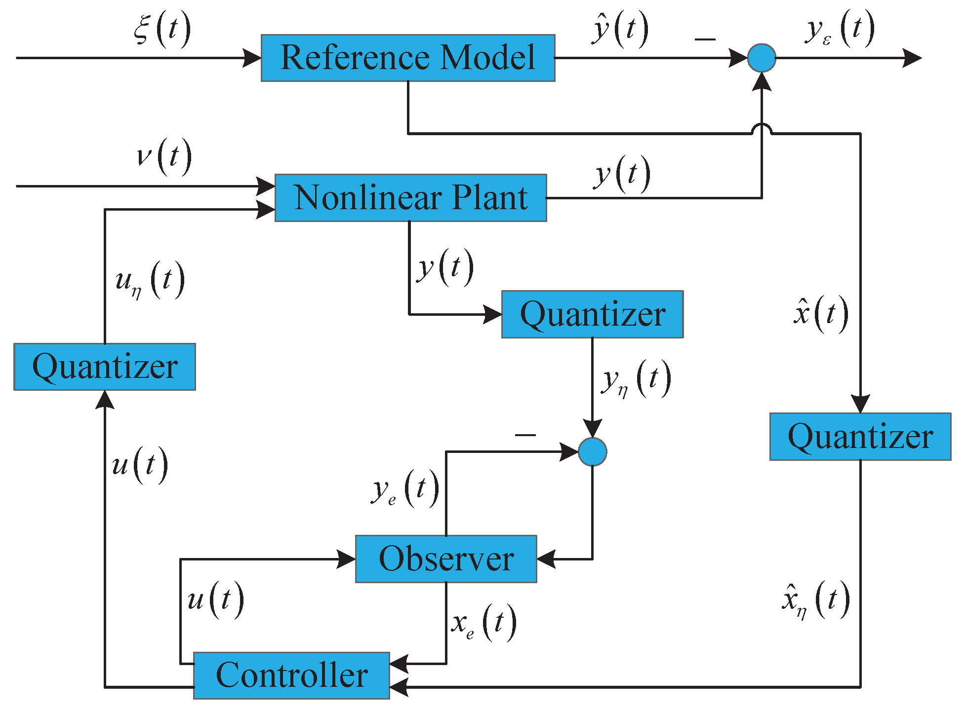
2.3. Observer-Based Output Feedback Tracking Controller

As in [10,12,15], the parallel distributed compensation strategy will be employed in this paper. In this case, the non-fragile observer for the fuzzy system in (4) can be constructed as

$$\begin{array}{c}{\dot{x}}_e\left(t\right)=A\left(\kappa \right)x_e\left(t\right)+B\left(\kappa \right)u\left(t\right)\hfill \\ +(L\left(\kappa \right)+{\beta }_L\left(t\right){\Xi }_L\left(\kappa \right))(y_{\eta }\left(t\right)-y_e\left(t\right))\hfill \\ y_e\left(t\right)=C\left(\kappa \right)x_e\left(t\right)\hfill \end{array}$$

(6)

where $x_e\left(t\right)\in {\mathbf{R}}^{n_x}$ denotes the state of the observer; $y_{\eta }\left(t\right)\in {\mathbf{R}}^{n_y}$ and $y_e\left(t\right)\in {\mathbf{R}}^{n_y}$ represent the quantized measured output of the plant and the output of the observer, respectively. $L\left(\kappa \right)={\displaystyle \sum _{q=1}^m}{\kappa }_q\left(\varsigma \left(t\right)\right)L_q,L_q\in {\mathbf{R}}^{n_x\times n_y},q=1,2,\dots ,m$ stand for the observer gains. ${\Xi }_L\left(\kappa \right)=X_L\left(\kappa \right){\Delta }_L\left(t\right)Y_L$ stands for the gain perturbation matrix, $X_L\left(\kappa \right)={\displaystyle \sum _{q=1}^m}{\kappa }_q\left(\varsigma \left(t\right)\right)X_{L_q}$ and $Y_L$ are given matrices; ${\Delta }_L\left(t\right)$ is an uncertain matrix and satisfies ${\Delta }_L^T\left(t\right){\Delta }_L\left(t\right)\le I$. ${\beta }_L\left(t\right)$ is a Bernoulli stochastic variable that satisfies

$$\begin{array}{c}Pr\{{\beta }_L\left(t\right)=1\}={\overline{\beta }}_L,Pr\{{\beta }_L\left(t\right)=0\}=1-{\overline{\beta }}_L\hfill \end{array}$$

where ${\overline{\beta }}_L=\mathbb{E}\left\{{\beta }_L\left(t\right)\right\}$ is a given constant.

The non-fragile observer-based tracking controller considered in this paper is given as follows:

$$\begin{array}{c}u\left(t\right)=\left(G\left(\kappa \right)+{\beta }_G\left(t\right){\Xi }_G\left(\kappa \right)\right)x_e\left(t\right)\hfill \\ +\left(S\left(\kappa \right)+{\beta }_S\left(t\right){\Xi }_S\left(\kappa \right)\right){\widehat{x}}_{\eta }\left(t\right)\hfill \end{array}$$

(7)

where $G\left(\kappa \right)={\displaystyle \sum _{q=1}^m}{\kappa }_q\left(\varsigma \left(t\right)\right)G_q,G_q\in {\mathbf{R}}^{n_u\times n_x},q=1,2,\dots ,m$, and $S\left(\kappa \right)={\displaystyle \sum _{q=1}^m}{\kappa }_q\left(\varsigma \left(t\right)\right)S_q,$$S_q\in {\mathbf{R}}^{n_u\times n_{\widehat{x}}},q=1,2,\dots ,m$ are the controller gains. ${\Xi }_G\left(\kappa \right)=X_G\left(\kappa \right){\Delta }_G\left(t\right)Y_G$ and ${\Xi }_S\left(\kappa \right)=X_S\left(\kappa \right){\Delta }_S\left(t\right)Y_S$ stand for the gain perturbation matrices, $X_G\left(\kappa \right)={\displaystyle \sum _{q=1}^m}{\kappa }_q\left(\varsigma \left(t\right)\right)X_{G_q}$, $X_S\left(\kappa \right)={\displaystyle \sum _{q=1}^m}{\kappa }_q\left(\varsigma \left(t\right)\right)X_{S_q}$, $Y_G$, and $Y_S$ are given matrices, ${\Delta }_G\left(t\right)$ and ${\Delta }_S\left(t\right)$ are uncertain matrices and satisfy ${\Delta }_G^T\left(t\right){\Delta }_G\left(t\right)\le I$ and ${\Delta }_S^T\left(t\right){\Delta }_S\left(t\right)\le I$, respectively. ${\beta }_G\left(t\right)$ and ${\beta }_S\left(t\right)$ are two independent Bernoulli stochastic variables that satisfy

$$\begin{array}{c}Pr\{{\beta }_G\left(t\right)=1\}={\overline{\beta }}_G,Pr\{{\beta }_G\left(t\right)=0\}={\overline{\beta }}_G\hfill \\ Pr\{{\beta }_S\left(t\right)=1\}={\overline{\beta }}_S,Pr\{{\beta }_S\left(t\right)=0\}={\overline{\beta }}_S\hfill \end{array}$$

where ${\overline{\beta }}_G=\mathbb{E}\left\{{\beta }_G\left(t\right)\right\}$ and ${\overline{\beta }}_S=\mathbb{E}\left\{{\beta }_S\left(t\right)\right\}$ are two given constants.

Remark 1. 

It should be noted that the observer-based tracking control scheme employed in this paper is more general than the one used in [32,33,35]. One of the main reasons for this is that the adopted observer in (6) and controller in (7) are non-fragile with randomly occurring gain variations. Furthermore, in order to simplify the analysis process, the control inputs of the observer and the system are often assumed to be the same in the study of observer-based output feedback tracking control for networked systems (see, e.g., [35]). However, the above assumption may not suit networked systems regarding the existence of the communication networks. In this paper, we consider that the control input of the observer in (6) and the control input of the system in (4) are different (see, Figure 1), which is a more general assumption in networked systems.

2.4. Dynamic Quantizers

In this paper, $u_{\eta }\left(t\right)$, $y_{\eta }\left(t\right)$, and ${\widehat{x}}_{\eta }\left(t\right)$ represent the quantized signals of $u\left(t\right)$, $y\left(t\right)$, and $\widehat{x}\left(t\right)$, i.e., the outputs of the following three dynamic quantizers, which are defined as

$$\begin{array}{c}{z}_{\eta }\left(t\right)=j_z\left(t\right){\eta }_z\left(\frac{z\left(t\right)}{j_z\left(t\right)}\right),z=u,y,\widehat{x}\hfill \end{array}$$

(8)

As in [5,6,7,8,9], $j_z\left(t\right)>0$ denotes a dynamic parameter and ${\eta }_z\left(z\left(t\right)/j_z\left(t\right)\right)$ stands for a static quantizer that satisfies

$$\mathrm{IF}\left|\frac{z\left(t\right)}{j_z\left(t\right)}\right|\le M_z,\mathrm{THEN}\left|{\eta }_z\left(\frac{z\left(t\right)}{j_z\left(t\right)}\right)-\frac{z\left(t\right)}{j_z\left(t\right)}\right|\le {\Delta }_z$$

(9)

$$\mathrm{IF}\left|\frac{z\left(t\right)}{j_z\left(t\right)}\right|>M_z,\mathrm{THEN}\left|{\eta }_z\left(\frac{z\left(t\right)}{j_z\left(t\right)}\right)\right|>M_z-{\Delta }_z$$

(10)

Here, ${\Delta }_z$ represents the quantization error bound and $M_z$ represents the quantization range of the quantizer ${\eta }_z\left(z\left(t\right)/j_z\left(t\right)\right)$.

Moreover, the quantized signals $u_{\eta }\left(t\right)$, $y_{\eta }\left(t\right)$, and ${\widehat{x}}_{\eta }\left(t\right)$ can be expressed as

$$\begin{array}{c}{z}_{\eta }\left(t\right)={\psi }_z\left(t\right)+z\left(t\right),z=u,y,\widehat{x}\hfill \end{array}$$

(11)

where ${\psi }_z\left(t\right)=j_z\left(t\right)\left({\eta }_z\left(\frac{z\left(t\right)}{j_z\left(t\right)}\right)-\frac{z\left(t\right)}{j_z\left(t\right)}\right)$.

Remark 2. 

In this paper, the dynamical quantization methodology developed in [5] is employed to reduce the data transmission burden of the communication network from the plant and the reference model to the controller and from the controller to the plant. Moreover, as pointed out in [9,23,40], an infinite number of quantization levels is necessary to guarantee the asymptotical stability of the resulting system in the static quantization methodology due to the inherent time-invariant quality of the static quantizer. In the dynamical quantization methodology considered in this paper, the quantization levels can be dynamically scaled to increase the region of attraction and reduce the steady-state limit cycle, which means that the asymptotical stability can be guaranteed under a finite number of quantization levels. As a result, in contrast with the static quantization methodology employed in [3,38,39] and references therein, the dynamical quantization methodology utilized in this paper is more general.

2.5. Resulting System

By substituting (11) into (4) and defining $x_{\varphi }\left(t\right)=x\left(t\right)-x_e\left(t\right)$,

$$\begin{array}{c}{\dot{x}}_{\varphi }\left(t\right)=(A\left(\kappa \right)-L\left(\kappa \right)C\left(\kappa \right)-{\beta }_L\left(t\right){\Xi }_L\left(\kappa \right)C\left(\kappa \right))x_{\varphi }\left(t\right)\hfill \\ -(L\left(\kappa \right)+{\beta }_L\left(t\right){\Xi }_L\left(\kappa \right)){\psi }_y\left(t\right)\hfill \\ +B\left(\kappa \right){\psi }_u\left(t\right)+D\left(\kappa \right)\nu \left(t\right)\hfill \end{array}$$

(12)

In order to utilize the descriptor representation strategy, we can rewrite the control input $u\left(t\right)$ as

$$\begin{array}{c}0·\dot{u}\left(t\right)=\left(G\left(\kappa \right)+{\beta }_G\left(t\right){\Xi }_G\left(\kappa \right)\right)x\left(t\right)-\left(G\left(\kappa \right)\right.\hfill \\ \left.+{\beta }_G\left(t\right){\Xi }_G\left(\kappa \right)\right)x_{\varphi }\left(t\right)+\left(S\left(\kappa \right)\right.\hfill \\ \left.+{\beta }_S\left(t\right){\Xi }_S\left(\kappa \right)\right){\widehat{x}}_{\eta }\left(t\right)-u\left(t\right)\hfill \end{array}$$

(13)

By defining ${\epsilon }^T\left(t\right)=\left[x^T\left(t\right)x_{\varphi }^T\left(t\right){\widehat{x}}^T\left(t\right)u^T\left(t\right)\right]$, ${\nu }_{\epsilon }^T\left(t\right)=\left[{\nu }^T\left(t\right){\xi }^T\left(t\right)\right]$, and $y_{\epsilon }\left(t\right)=y\left(t\right)-\widehat{y}\left(t\right)$, the resulting system in the descriptor form can be represented as follows:

$$\begin{array}{c}\mathbf{E}\dot{\epsilon }\left(t\right)=\left({\widehat{A}}_a+{\widehat{\beta }}_L\left(t\right){\widehat{A}}_b+{\widehat{\beta }}_G\left(t\right){\widehat{A}}_c+{\widehat{\beta }}_S\left(t\right){\widehat{A}}_d\right)\hfill \\ \times \epsilon \left(t\right)+\left(Q_y+{\widehat{\beta }}_L\left(t\right){\widehat{Q}}_y\right){\psi }_y\left(t\right)+(Q_{\widehat{x}}\hfill \\ \left.+{\widehat{\beta }}_S\left(t\right){\widehat{Q}}_{\widehat{x}}\right){\psi }_{\widehat{x}}\left(t\right)+Q_u{\psi }_u\left(t\right)+\widehat{B}{\nu }_{\epsilon }\left(t\right)\hfill \\ y_{\epsilon }\left(t\right)=\widehat{C}\epsilon \left(t\right)\hfill \end{array}$$

(14)

where ${\widehat{\beta }}_L\left(t\right)={\beta }_L\left(t\right)-{\overline{\beta }}_L$, ${\widehat{\beta }}_G\left(t\right)={\beta }_G\left(t\right)-{\overline{\beta }}_G$, ${\widehat{\beta }}_S\left(t\right)={\beta }_S\left(t\right)-{\overline{\beta }}_S$, $\widehat{C}=[C\left(\kappa \right)0-C_{\xi }0]$, and

$$\begin{array}{c}\mathbf{E}=\left[\begin{array}{cccc}I& 0& 0& 0\\ 0& I& 0& 0\\ 0& 0& I& 0\\ 0& 0& 0& 0\end{array}\right],Q_y=\left[\begin{array}{c}0\\ -L\left(\kappa \right)-{\overline{\beta }}_L{\Xi }_L\left(\kappa \right)\\ 0\\ 0\end{array}\right],Q_u=\left[\begin{array}{c}B\left(\kappa \right)\\ B\left(\kappa \right)\\ 0\\ 0\end{array}\right],\hfill \\ {\widehat{A}}_a=\left[\begin{array}{cccc}A\left(\kappa \right)& 0& 0& B\left(\kappa \right)\\ 0& {\theta }_{22}& 0& 0\\ 0& 0& A_{\xi }& 0\\ {\theta }_{41}& -{\theta }_{41}& {\theta }_{43}& -I\end{array}\right],{\widehat{Q}}_{\widehat{x}}=\left[\begin{array}{c}0\\ 0\\ 0\\ {\Xi }_S\left(\kappa \right)\end{array}\right],\hfill \\ {\widehat{A}}_b=\left[\begin{array}{cccc}0& 0& 0& 0\\ 0& -{\Xi }_L\left(\kappa \right)C\left(\kappa \right)& 0& 0\\ 0& 0& 0& 0\\ 0& 0& 0& 0\end{array}\right],{\widehat{Q}}_y=\left[\begin{array}{c}0\\ -{\Xi }_L\left(\kappa \right)\\ 0\\ 0\end{array}\right],\hfill \\ {\widehat{A}}_c=\left[\begin{array}{cccc}0& 0& 0& 0\\ 0& 0& 0& 0\\ 0& 0& 0& 0\\ {\Xi }_G\left(\kappa \right)& -{\Xi }_G\left(\kappa \right)& 0& 0\end{array}\right],\widehat{B}=\left[\begin{array}{cc}D\left(\kappa \right)& 0\\ D\left(\kappa \right)& 0\\ 0& B_{\xi }\\ 0& 0\end{array}\right],\hfill \\ {\widehat{A}}_d=\left[\begin{array}{cccc}0& 0& 0& 0\\ 0& 0& 0& 0\\ 0& 0& 0& 0\\ 0& 0& {\Xi }_S\left(\kappa \right)& 0\end{array}\right],Q_{\widehat{x}}=\left[\begin{array}{c}0\\ 0\\ 0\\ S\left(\kappa \right)+{\overline{\beta }}_S{\Xi }_S\left(\kappa \right)\end{array}\right],\hfill \end{array}$$

$${\theta }_{22}=A\left(\kappa \right)-L\left(\kappa \right)C\left(\kappa \right)-{\overline{\beta }}_L{\Xi }_L\left(\kappa \right)C\left(\kappa \right),{\theta }_{41}=G\left(\kappa \right)+{\overline{\beta }}_G{\Xi }_G\left(\kappa \right),{\theta }_{43}=S\left(\kappa \right)+{\overline{\beta }}_S{\Xi }_S\left(\kappa \right).$$

Before we present the objective of this paper, the following definition will be given.

Definition 1 

([16]). It can be concluded that the resulting system (14) is asymptotically stable in the mean-square sense, if

$$\underset{t\to \infty }{lim}\mathbb{E}\left\{{\left|\epsilon \left(t\right)\right|}^2\right\}=0$$

is satisfied for any initial conditions with ${\nu }_{\epsilon }\left(t\right)=0$.

The purpose of this paper is to design the non-fragile observer in (6), the non-fragile tracking controller in (7), and the dynamic quantizers in (8) such that the resulting system in (14) satisfies the following two tracking requirements.

(1) The resulting system in (14) is mean-square asymptotically stable with ${\nu }_{\epsilon }\left(t\right)=0$.

(2) The given ${\mathcal{H}}_{\infty }$ tracking performance $\sigma >0$ can be guaranteed for all ${\nu }_{\epsilon }\left(t\right)\ne 0$ with the zero-initial conditions, i.e., the tracking error $y_{\epsilon }\left(t\right)$ satisfies

$${\int }_0^{t_r}{y}_{\epsilon }^T\left(t\right)y_{\epsilon }\left(t\right)dt<{\sigma }^2{\int }_0^{t_r}{\nu }_{\epsilon }^T\left(t\right){\nu }_{\epsilon }\left(t\right)dt$$

where $t_r>0$ is the final time.

The following lemma plays a critical role in deriving the central results of this paper.

Lemma 1 

([17,20]). For real matrices ${\mathbf{X}}_0={\mathbf{X}}_0^T$, ${\mathbf{X}}_1$, ${\mathbf{X}}_2$, and ${\mathbf{X}}_3$ with appropriate dimensions, then, we can obtain that ${\mathbf{X}}_0+{\mathbf{X}}_1{\mathbf{X}}_2{\mathbf{X}}_3+{\mathbf{X}}_3^T{\mathbf{X}}_2^T{\mathbf{X}}_1^T<0$ is true for all ${\mathbf{X}}_2^T{\mathbf{X}}_2\le I$, if and only if ${\mathbf{X}}_0+d^{-1}{\mathbf{X}}_1{\mathbf{X}}_1^T+d{\mathbf{X}}_3^T{\mathbf{X}}_3<0$ is satisfied for a positive scalar $d>0$.

3. Main Results

3.1. Tracking Performance Analysis

In this subsection, the problem of ${\mathcal{H}}_{\infty }$ tracking performance analysis will be addressed. More specifically, we assume that the gains in the non-fragile observer in (6) and the non-fragile tracking controller in (7) are known; then, the sufficient conditions will be established in the following theorem to ensure the mean-square asymptotical stability and the given ${\mathcal{H}}_{\infty }$ tracking performance for the resulting system in (14).

Theorem 1. 

Consider the fuzzy system in (4), the reference model in (5), the observer-based non-fragile tracking controller in (7), and the dynamic quantizers in (8). For given scalars ${\overline{\beta }}_L$, ${\overline{\beta }}_G$, ${\overline{\beta }}_S$, ${\Delta }_z$, and $M_z$, $z=u,y,\widehat{x}$, the resulting system in (14) is asymptotically stable in the mean-square sense and the prescribed ${\mathcal{H}}_{\infty }$ performance $\sigma >0$ can be guaranteed with the online adjusting strategies for the dynamic parameters $j_z\left(t\right)$ as

$$f_z\left|z\left(t\right)\right|\le j_z\left(t\right)\le 2f_z\left|z\left(t\right)\right|,z=u,y,\widehat{x}.$$

(15)

If there exist matrix $P>0$ and scalars $b_z>0$, $f_z>0$ satisfying

$$M_z-1/f_z>0,z=u,y,\widehat{x}$$

(16)

$$P\mathbf{E}={\mathbf{E}}^T{P}^T\ge 0$$

(17)

$$\left[\begin{array}{cc}{\mathcal{Z}}_{11}& *\\ {\mathcal{Z}}_{21}& {\mathcal{Z}}_{22}\end{array}\right]<0$$

(18)

where ${\mathcal{Z}}_{11}=P{\widehat{A}}_a+{\widehat{A}}_a^T{P}^T+{\widehat{C}}^T\widehat{C}$,

$$\begin{array}{c}{\mathcal{Z}}_{21}={\left[P{Q}_{y}P{Q}_{\widehat{x}}P{Q}_{u}P\widehat{B}{b}_y{\Sigma }_y^T{b}_{\widehat{x}}{\Sigma }_{\widehat{x}}^T{b}_u{\Sigma }_u^T\right]}^T,\hfill \\ {\mathcal{Z}}_{22}=-daig\left\{b_{y}I,b_{\widehat{x}}I,b_{u}I,{\sigma }^{2}I,b_{y}I,b_{\widehat{x}}I,b_{u}I\right\},\hfill \end{array}$$

${\Sigma }_u=\left[0002f_u{\Delta }_{u}I\right]$, ${\Sigma }_y=\left[2f_y{\Delta }_{y}C\left(\kappa \right)000\right]$, and ${\Sigma }_{\widehat{x}}=\left[002f_{\widehat{x}}{\Delta }_{\widehat{x}}I0\right]$.

Proof. 

Firstly, for ${\nu }_{\epsilon }\left(t\right)=0$, we will show that the resulting system in (14) is mean-square asymptotically stable with the online adjusting strategies in (15) if the conditions in (16)–(18) are satisfied.

Based on the results proposed in [23,28], the following inequalities can be obtained from (9), (15), and (16):

$$4f_z^2{\Delta }_z^2{z}^T\left(t\right)z\left(t\right)-{\psi }_z^T\left(t\right){\psi }_z\left(t\right)\ge 0,z=u,y,\widehat{x}$$

(19)

which can be expressed as

$${\tilde{\epsilon }}^T\left(t\right){\widehat{\mathcal{H}}}_z\tilde{\epsilon }\left(t\right)\ge 0,z=u,y,\widehat{x}$$

(20)

where $\tilde{\epsilon }\left(t\right)={\left[{\epsilon }^T\left(t\right){\psi }_y^T\left(t\right){\psi }_{\widehat{x}}^T\left(t\right){\psi }_u^T\left(t\right)\right]}^T$,

$$\begin{array}{c}{\widehat{\mathcal{H}}}_u={\left[{\Sigma }_{u}000\right]}^T\left[{\Sigma }_{u}000\right]-daig\left\{0,0,0,I\right\},\hfill \\ {\widehat{\mathcal{H}}}_y={\left[{\Sigma }_{y}000\right]}^T\left[{\Sigma }_{y}000\right]-daig\left\{0,I,0,0\right\},\hfill \\ {\widehat{\mathcal{H}}}_{\widehat{x}}={\left[{\Sigma }_{\widehat{x}}000\right]}^T\left[{\Sigma }_{\widehat{x}}000\right]-daig\left\{0,0,I,0\right\}.\hfill \end{array}$$

For the resulting system (14), the Lyapunov function can be formulated as

$$V\left(\epsilon \left(t\right)\right)={\epsilon }^T\left(t\right)P\mathbf{E}\epsilon \left(t\right),P\mathbf{E}={\mathbf{E}}^T{P}^T\ge 0$$

(21)

then, we have

$$\begin{array}{c}\mathbb{E}\left\{\dot{V}\left(\epsilon \left(t\right)\right)\right\}\hfill \\ =\mathbb{E}\left\{{\epsilon }^T\left(t\right)P\mathbf{E}\dot{\epsilon }\left(t\right)+{\dot{\epsilon }}^T\left(t\right){\mathbf{E}}^T{P}^T\epsilon \left(t\right)\right\}\hfill \\ =\mathbb{E}\left\{{\epsilon }^T\left(t\right)P\left(\left({\widehat{A}}_a+{\widehat{\beta }}_L\left(t\right){\widehat{A}}_b+{\widehat{\beta }}_G\left(t\right){\widehat{A}}_c+{\widehat{\beta }}_S\left(t\right){\widehat{A}}_d\right)\right.\right.\hfill \\ \times \epsilon \left(t\right)+\left(Q_y+{\widehat{\beta }}_L\left(t\right){\widehat{Q}}_y\right){\psi }_y\left(t\right)+\left(Q_{\widehat{x}}+{\widehat{\beta }}_S\left(t\right){\widehat{Q}}_{\widehat{x}}\right)\hfill \\ \times {\psi }_{\widehat{x}}\left(t\right)+Q_u{\psi }_u\left(t\right))+\left(\left({\widehat{A}}_a+{\widehat{\beta }}_L\left(t\right){\widehat{A}}_b+{\widehat{\beta }}_G\left(t\right){\widehat{A}}_c\right.\right.\hfill \\ \left.+{\widehat{\beta }}_S\left(t\right){\widehat{A}}_d\right)\epsilon \left(t\right)+\left(Q_y+{\widehat{\beta }}_L\left(t\right){\widehat{Q}}_y\right){\psi }_y\left(t\right)+(Q_{\widehat{x}}\hfill \\ \left.+{\widehat{\beta }}_S\left(t\right){\widehat{Q}}_{\widehat{x}}\right){\psi }_{\widehat{x}}\left(t\right)+Q_u{\psi }_u\left(t\right){)}^T{P}^T\epsilon \left(t\right)\}\hfill \\ ={\epsilon }^T\left(t\right)P\left({\widehat{A}}_a\epsilon \left(t\right)+Q_y{\psi }_y\left(t\right)+Q_{\widehat{x}}{\psi }_{\widehat{x}}\left(t\right)+Q_u{\psi }_u\left(t\right)\right)\hfill \\ +{\left({\widehat{A}}_a\epsilon \left(t\right)+Q_y{\psi }_y\left(t\right)+Q_{\widehat{x}}{\psi }_{\widehat{x}}\left(t\right)+Q_u{\psi }_u\left(t\right)\right)}^T{P}^T\epsilon \left(t\right)\hfill \\ ={\tilde{\epsilon }}^T\left(t\right){\widehat{\mathcal{H}}}_c\tilde{\epsilon }\left(t\right)\hfill \end{array}$$

(22)

where ${\widehat{\mathcal{H}}}_c=He\left\{{\left[{\widehat{A}}_a{Q}_y{Q}_{\widehat{x}}{Q}_u\right]}^T\left[P^{T}000\right]\right\}$.

For ${\nu }_{\epsilon }\left(t\right)=0$, the following inequality can be obtained according to (18), which is given as

$$\left[\begin{array}{cc}{\widehat{\mathcal{Z}}}_{11}& *\\ {\widehat{\mathcal{Z}}}_{21}& {\widehat{\mathcal{Z}}}_{22}\end{array}\right]<0$$

(23)

where ${\widehat{\mathcal{Z}}}_{11}=P{\widehat{A}}_a+{\widehat{A}}_a^T{P}^T$,

$$\begin{array}{c}{\widehat{\mathcal{Z}}}_{21}={\left[P{Q}_{y}P{Q}_{\widehat{x}}P{Q}_u{b}_y{\Sigma }_y^T{b}_{\widehat{x}}{\Sigma }_{\widehat{x}}^T{b}_u{\Sigma }_u^T\right]}^T,\hfill \\ {\widehat{\mathcal{Z}}}_{22}=-daig\left\{b_{y}I,b_{\widehat{x}}I,b_{u}I,b_{y}I,b_{\widehat{x}}I,b_{u}I\right\}.\hfill \end{array}$$

Performing congruence transformation to (23) by $daig\left\{I,\widehat{\mathcal{X}}\right\}$ with $\widehat{\mathcal{X}}=daig\left\{I,I,I,\right.$$\left.b_y^{-1}I,b_{\widehat{x}}^{-1}I,b_u^{-1}I\right\}$ and utilizing the Schur complement, we can obtain that

$${\widehat{\mathcal{H}}}_c+b_y{\widehat{\mathcal{H}}}_y+b_{\widehat{x}}{\widehat{\mathcal{H}}}_{\widehat{x}}+b_u{\widehat{\mathcal{H}}}_u<0$$

(24)

Then, based on the S-procedure in [9,27], one can conclude that

$$\mathbb{E}\left\{\dot{V}\left(\epsilon \left(t\right)\right)\right\}={\tilde{\epsilon }}^T\left(t\right){\widehat{\mathcal{H}}}_c\tilde{\epsilon }\left(t\right)<0$$

(25)

Moreover, according to Definition 1 and the results developed in [16], we can deduce that the resulting system in (14) is asymptotically stable in the mean square for ${\nu }_{\epsilon }\left(t\right)=0$.

Next, for all ${\nu }_{\epsilon }\left(t\right)\ne 0$, the ${\mathcal{H}}_{\infty }$ tracking performance of the resulting system (14) will be established with zero initial conditions.

For ${\nu }_{\epsilon }\left(t\right)\ne 0$, the inequalities given in (20) can be indicated as

$${\widehat{\epsilon }}^T\left(t\right){\mathcal{H}}_z\widehat{\epsilon }\ge 0,z=u,y,\widehat{x}$$

(26)

where $\widehat{\epsilon }\left(t\right)={\left[{\epsilon }^T\left(t\right){\psi }_y^T\left(t\right){\psi }_{\widehat{x}}^T\left(t\right){\psi }_u^T\left(t\right){\nu }_{\epsilon }^T\left(t\right)\right]}^T$,

$$\begin{array}{c}{\widehat{\mathcal{H}}}_u={\left[{\Sigma }_{u}0000\right]}^T\left[{\Sigma }_{u}0000\right]-daig\left\{0,0,0,I,0\right\},\hfill \\ {\widehat{\mathcal{H}}}_y={\left[{\Sigma }_{y}0000\right]}^T\left[{\Sigma }_{y}0000\right]-daig\left\{0,I,0,0,0\right\},\hfill \\ {\widehat{\mathcal{H}}}_{\widehat{x}}={\left[{\Sigma }_{\widehat{x}}0000\right]}^T\left[{\Sigma }_{\widehat{x}}0000\right]-daig\left\{0,0,I,0,0\right\}.\hfill \end{array}$$

Then, we have

$$\begin{array}{c}\mathbb{E}\left\{\dot{V}\left(\epsilon \left(t\right)\right)\right\}+y_{\epsilon }^T\left(t\right)y_{\epsilon }\left(t\right)-{\sigma }^2{\nu }_{\epsilon }^T\left(t\right){\nu }_{\epsilon }\left(t\right)\hfill \\ =\mathbb{E}\left\{{\epsilon }^T\left(t\right)P\left(\left({\widehat{A}}_a+{\widehat{\beta }}_L\left(t\right){\widehat{A}}_b+{\widehat{\beta }}_G\left(t\right){\widehat{A}}_c+{\widehat{\beta }}_S\left(t\right){\widehat{A}}_d\right)\right.\right.\hfill \\ \times \epsilon \left(t\right)+\left(Q_y+{\widehat{\beta }}_L\left(t\right){\widehat{Q}}_y\right){\psi }_y\left(t\right)+\left(Q_{\widehat{x}}+{\widehat{\beta }}_S\left(t\right){\widehat{Q}}_{\widehat{x}}\right)\hfill \\ \times {\psi }_{\widehat{x}}\left(t\right)+Q_u{\psi }_u\left(t\right)+\widehat{B}{\nu }_{\epsilon }\left(t\right))+\left(\left({\widehat{A}}_a+{\widehat{\beta }}_L\left(t\right){\widehat{A}}_b\right.\right.\hfill \\ \left.+{\widehat{\beta }}_G\left(t\right){\widehat{A}}_c+{\widehat{\beta }}_S\left(t\right){\widehat{A}}_d\right)\epsilon \left(t\right)+\left(Q_y+{\widehat{\beta }}_L\left(t\right){\widehat{Q}}_y\right){\psi }_y\left(t\right)\hfill \\ +\left(Q_{\widehat{x}}+{\widehat{\beta }}_S\left(t\right){\widehat{Q}}_{\widehat{x}}\right){\psi }_{\widehat{x}}\left(t\right)+Q_u{\psi }_u\left(t\right)+\widehat{B}{\nu }_{\epsilon }\left(t\right){)}^T\hfill \\ \times P^T\epsilon \left(t\right)\}+{\epsilon }^T\left(t\right){\widehat{C}}^T\widehat{C}\epsilon \left(t\right)-{\sigma }^2{\nu }_{\epsilon }^T\left(t\right){\nu }_{\epsilon }\left(t\right)\hfill \\ ={\epsilon }^T\left(t\right)P\left({\widehat{A}}_a\epsilon \left(t\right)+Q_y{\psi }_y\left(t\right)+Q_{\widehat{x}}{\psi }_{\widehat{x}}\left(t\right)+Q_u{\psi }_u\left(t\right)\right.\hfill \\ +\widehat{B}{\nu }_{\epsilon }\left(t\right))+\left({\widehat{A}}_a\epsilon \left(t\right)+Q_y{\psi }_y\left(t\right)+Q_{\widehat{x}}{\psi }_{\widehat{x}}\left(t\right)+Q_u\right.\hfill \\ {\left.\times {\psi }_u\left(t\right)+\widehat{B}{\nu }_{\epsilon }\left(t\right)\right)}^T{P}^T\epsilon \left(t\right)+{\epsilon }^T\left(t\right){\widehat{C}}^T\widehat{C}\epsilon \left(t\right)\hfill \\ -{\sigma }^2{\nu }_{\epsilon }^T\left(t\right){\nu }_{\epsilon }\left(t\right)\hfill \\ ={\widehat{\epsilon }}^T\left(t\right){\mathcal{H}}_c\widehat{\epsilon }\left(t\right)\hfill \end{array}$$

(27)

where ${\mathcal{H}}_c=He\left\{{\left[{\widehat{A}}_a{Q}_y{Q}_{\widehat{x}}{Q}_u\widehat{B}\right]}^T\left[P^{T}0000\right]\right\}+diag\left\{{\widehat{C}}^T\widehat{C},0,0,0-{\sigma }^{2}I\right\}$.

Let us perform congruence transformation to (18) by $daig\left\{I,\mathcal{X}\right\}$ with $\mathcal{X}=daig\left\{I,I,I,\right.$$\left.I,b_y^{-1}I,b_{\widehat{x}}^{-1}I,b_u^{-1}I\right\}$ and utilize the Schur complement; this shows that

$${\mathcal{H}}_c+b_y{\mathcal{H}}_y+b_{\widehat{x}}{\mathcal{H}}_{\widehat{x}}+b_u{\mathcal{H}}_u<0$$

(28)

Then, based on the S-procedure in [9,27], we have that ${\widehat{\epsilon }}^T\left(t\right){\mathcal{H}}_c\widehat{\epsilon }\left(t\right)<0$, i.e.,

$$\begin{array}{c}\mathbb{E}\left\{\dot{V}\left(\epsilon \left(t\right)\right)\right\}+y_{\epsilon }^T\left(t\right)y_{\epsilon }\left(t\right)-{\sigma }^2{\nu }_{\epsilon }^T\left(t\right){\nu }_{\epsilon }\left(t\right)<0\hfill \end{array}$$

(29)

By integrating (29) from 0 to $t_r$, we obtain that

$$\begin{array}{c}{\int }_0^{t_r}\mathbb{E}\left\{\dot{V}\left(\epsilon \left(t\right)\right)\right\}dt+{\int }_0^{t_r}{y}_{\epsilon }^T\left(t\right)y_{\epsilon }\left(t\right)dt\hfill \\ -{\sigma }^2{\int }_0^{t_r}{\nu }_{\epsilon }^T\left(t\right){\nu }_{\epsilon }\left(t\right)dt\hfill \\ =\mathbb{E}\left\{\dot{V}\left(\epsilon \left(t_r\right)\right)\right\}-\mathbb{E}\left\{\dot{V}\left(\epsilon \left(0\right)\right)\right\}\hfill \\ +{\int }_0^{t_r}{y}_{\epsilon }^T\left(t\right)y_{\epsilon }\left(t\right)dt-{\sigma }^2{\int }_0^{t_r}{\nu }_{\epsilon }^T\left(t\right){\nu }_{\epsilon }\left(t\right)dt<0\hfill \end{array}$$

(30)

Consider the zero initial conditions and $\mathbb{E}\left\{\dot{V}\left(\epsilon \left(t_r\right)\right)\right\}\ge 0$, we can obtain that

$${\int }_0^{t_r}{y}_{\epsilon }^T\left(t\right)y_{\epsilon }\left(t\right)dt<{\sigma }^2{\int }_0^{t_r}{\nu }_{\epsilon }^T\left(t\right){\nu }_{\epsilon }\left(t\right)dt.$$

It is shown that the ${\mathcal{H}}_{\infty }$ tracking performance of the resulting system (14) can be guaranteed.

The proof is completed. □

3.2. Non-Fragile Tracking Controller Design

In the following theorem, based on the ${\mathcal{H}}_{\infty }$ tracking performance analysis criterion developed in Theorem 1, a co-design strategy for the desired non-fragile observer in (6), the tracking controller in (7), and dynamic quantizers in (8) will be proposed in terms of linear matrix inequalities.

Theorem 2. 

Consider the fuzzy system in (4), the reference model in (5), the observer-based non-fragile tracking controller in (7), and the dynamic quantizers in (8). For given scalars ${\overline{\beta }}_L$, ${\overline{\beta }}_G$, ${\overline{\beta }}_S$, ${\Delta }_z$, and $M_z$, $z=u,y,\widehat{x}$, the resulting system in (14) is asymptotically stable in the mean-square sense and the prescribed ${\mathcal{H}}_{\infty }$ performance $\sigma >0$ can be guaranteed with the online adjusting strategies for the dynamic parameters $j_z\left(t\right)$ defined in (15) subject to $f_z=g_z/b_z$. If there exist scalars $b_z>0$, $g_z>0$, $d_L>0$, $d_G>0$, $d_S>0$ and matrices $P_{11}>0$, $P_{22}>0$, $P_{33}>0$, $P_{44}$, ${\widehat{L}}_q$, ${\widehat{G}}_q$, ${\widehat{S}}_q$ for $q=1,2,\dots ,m$ satisfying

$$g_z{M}_z-b_z>0,z=u,y,\widehat{x}$$

(31)

$$\left[\begin{array}{ccc}{P}_{11}& *& *\\ P_{22}& P_{22}& *\\ 0& 0& P_{33}\end{array}\right]>0$$

(32)

$$T_{ll}<0,l=1,2,\cdots ,m$$

(33)

$$T_{lq}+T_{ql}<0,l,q=1,2,\cdots ,m,l<q$$

(34)

where

$$\begin{array}{c}{T}_{lq}=\left[\begin{array}{ccccccc}{\mathcal{T}}_{11}^{lq}& *& *& *& *& *& *\\ {\mathcal{T}}_{21}^{lq}& {\mathcal{T}}_{22}& *& *& *& *& *\\ {\mathcal{T}}_{31}^l& 0& -{\sigma }^{2}I& *& *& *& *\\ {\mathcal{T}}_{41}^l& 0& 0& {\mathcal{T}}_{22}& *& *& *\\ {\mathcal{T}}_{51}^{lq}& {\mathcal{T}}_{52}& 0& 0& -d_{L}I& *& *\\ {\mathcal{T}}_{61}^q& 0& 0& 0& 0& -d_{G}I& *\\ {\mathcal{T}}_{71}^q& {\mathcal{T}}_{72}& 0& 0& 0& 0& -d_{S}I\end{array}\right],\hfill \\ {\mathcal{T}}_{11}^{lq}=\left[\begin{array}{cccc}{\Theta }_{1l}& *& *& *\\ {\Theta }_{2lq}& {\Theta }_{3lq}& *& *\\ -C_{\xi }^T{C}_l& 0& {\Theta }_4& *\\ {\Theta }_{5lq}& {\Theta }_{6lq}& {\widehat{S}}_q& -He\left\{P_{44}\right\}\end{array}\right],\hfill \end{array}$$

$$\begin{array}{c}{\mathcal{T}}_{21}^{lq}=\left[\begin{array}{cccc}-{\widehat{L}}_q^T& -{\widehat{L}}_q^T& 0& 0\\ 0& 0& 0& {\widehat{S}}_q^T\\ {\Theta }_{7l}& 2B_l^T{P}_{22}^T& 0& 0\end{array}\right],\hfill \\ {\mathcal{T}}_{22}=-daig\left\{b_{y}I,b_{\widehat{x}}I,b_{u}I\right\},\hfill \\ {\mathcal{T}}_{31}^l=\left[\begin{array}{cccc}{\Theta }_{8l}& 2D_l^T{P}_{22}^T& 0& 0\\ 0& 0& B_{\xi }^T{P}_{33}^T& 0\end{array}\right],\hfill \\ {\mathcal{T}}_{41}^l=\left[\begin{array}{cccc}2g_y{\Delta }_y{C}_l& 0& 0& 0\\ 0& 0& 2g_{\widehat{x}}{\Delta }_{\widehat{x}}I& 0\\ 0& 0& 0& 2g_u{\Delta }_{u}I\end{array}\right],\hfill \\ {\mathcal{T}}_{51}^{lq}=\left[\begin{array}{cccc}-{\overline{\beta }}_L{X}_{L_q}^T{P}_{22}^T& -{\overline{\beta }}_L{X}_{L_q}^T{P}_{22}^T& 0& 0\\ 0& d_L{Y}_L{C}_l& 0& 0\end{array}\right],\hfill \\ {\mathcal{T}}_{52}=\left[\begin{array}{ccc}0& 0& 0\\ d_L{Y}_L& 0& 0\end{array}\right],\hfill \\ {\mathcal{T}}_{61}^q=\left[\begin{array}{cccc}0& 0& 0& {\overline{\beta }}_G{X}_{G_q}^T{P}_{44}^T\\ d_G{Y}_G& -d_G{Y}_G& 0& 0\end{array}\right],\hfill \\ {\mathcal{T}}_{71}^q=\left[\begin{array}{cccc}0& 0& 0& {\overline{\beta }}_S{X}_{S_q}^T{P}_{44}^T\\ 0& 0& d_S{Y}_S& 0\end{array}\right],\hfill \\ {\mathcal{T}}_{72}=\left[\begin{array}{ccc}0& 0& 0\\ 0& d_S{Y}_S& 0\end{array}\right],\hfill \end{array}$$

${\Theta }_{1l}=He\left\{P_{11}{A}_l\right\}+C_l^T{C}_l$, ${\Theta }_{2lq}=He\left\{P_{22}{A}_l\right\}-C_l^T{\widehat{L}}_q^T$, ${\Theta }_{3lq}=He\{P_{22}{A}_l-{\widehat{L}}_q{C}_l\}$, ${\Theta }_4=He\left\{P_{33}{A}_{\xi }\right\}+C_{\xi }^T{C}_{\xi }$, ${\Theta }_{5lq}=B_l^T{P}_{11}^T+{\widehat{G}}_q$, ${\Theta }_{6lq}=B_l^T{P}_{22}^T-{\widehat{G}}_q$, ${\Theta }_{7l}=B_l^T{P}_{11}^T+B_l^T{P}_{22}^T$, ${\Theta }_{8l}=D_l^T{P}_{11}^T+D_l^T{P}_{22}^T$.

Furthermore, the desired gains for the non-fragile observer in (6) and the non-fragile tracking controller in (7) can be obtained as

$$L_q=P_{22}^{-1}{\widehat{L}}_q,G_q=P_{44}^{-1}{\widehat{G}}_q,S_q=P_{44}^{-1}{\widehat{S}}_q.$$

(35)

Proof. 

The condition of (18) developed in Theorem 1 can be expressed as

$$\begin{array}{c}{\Pi }_1+He\left\{{\Psi }_1{\Delta }_L\left(t\right){\Psi }_2+{\Psi }_3{\Delta }_G\left(t\right){\Psi }_4+{\Psi }_5{\Delta }_S\left(t\right){\Psi }_6\right\}<0\hfill \end{array}$$

(36)

where

$$\begin{array}{c}{\Pi }_1=\left[\begin{array}{cccc}{S}_{11}& *& *& *\\ S_{21}& {\mathcal{T}}_{22}& *& *\\ S_{31}& 0& -{\sigma }^{2}I& *\\ S_{41}& 0& 0& {\mathcal{T}}_{22}\end{array}\right],\hfill \end{array}$$

${\Psi }_1={\left[R_1^T{P}^{T}000\right]}^T$, ${\Psi }_2=\left[R_2{R}_{3}00\right]$, ${\Psi }_3={\left[R_4^T{P}^{T}000\right]}^T$, ${\Psi }_4=\left[R_{5}000\right]$, ${\Psi }_5={\left[R_6^T{P}^{T}000\right]}^T$, ${\Psi }_6=\left[R_7{R}_{8}00\right]$, $S_{11}=P{\overline{A}}_a+{\overline{A}}_a^T{P}^T+{\widehat{C}}^T\widehat{C}$, $S_{21}={\left[P{\overline{Q}}_{y}P{\overline{Q}}_{\widehat{x}}P{Q}_u\right]}^T$, $S_{31}={\widehat{B}}^T{P}^T$, $S_{41}={\left[b_y{\Sigma }_y^T{b}_{\widehat{x}}{\Sigma }_{\widehat{x}}^T{b}_u{\Sigma }_u^T\right]}^T$, $R_1^T=[0-{\overline{\beta }}_L{X}_L^T\left(\kappa \right)00]$, $R_2=\left[0Y_{L}C\left(\kappa \right)00\right]$, $R_3=\left[Y_{L}00\right]$, $R_4^T=\left[000{\overline{\beta }}_G{X}_G^T\left(\kappa \right)\right]$, $R_5=[Y_G-Y_{G}00]$, $R_6^T=\left[000{\overline{\beta }}_S{X}_S^T\left(\kappa \right)\right]$, $R_7=\left[00Y_{S}0\right]$, $R_8=\left[0Y_{S}0\right]$, ${\overline{Q}}_y={[0-L^T\left(\kappa \right)00]}^T$, ${\overline{Q}}_{\widehat{x}}={\left[000S^T\left(\kappa \right)\right]}^T$,

$${\overline{A}}_a=\left[\begin{array}{cccc}A\left(\kappa \right)& 0& 0& B\left(\kappa \right)\\ 0& A\left(\kappa \right)-L\left(\kappa \right)C\left(\kappa \right)& 0& 0\\ 0& 0& A_{\xi }& 0\\ G\left(\kappa \right)& -G\left(\kappa \right)& S\left(\kappa \right)& -I\end{array}\right].$$

Then, according to Lemma 1 and the Schur complement, it can be obtained that the inequality in (36) holds if, for positive scalars $d_L$, $d_G$, and $d_S$,

$$\left[\begin{array}{ccccccc}{S}_{11}& *& *& *& *& *& *\\ S_{21}& {\mathcal{T}}_{22}& *& *& *& *& *\\ S_{31}& 0& -{\sigma }^{2}I& *& *& *& *\\ S_{41}& 0& 0& {\mathcal{T}}_{22}& *& *& *\\ S_{51}& {\mathcal{T}}_{52}& 0& 0& -d_{L}I& *& *\\ S_{61}& 0& 0& 0& 0& -d_{G}I& *\\ S_{71}& {\mathcal{T}}_{72}& 0& 0& 0& 0& -d_{S}I\end{array}\right]<0$$

(37)

where

$$\begin{array}{c}{S}_{51}=\left[\begin{array}{c}{R}_1^T{P}^T\\ d_L{R}_2\end{array}\right],S_{61}=\left[\begin{array}{c}{R}_4^T{P}^T\\ d_G{R}_5\end{array}\right],S_{71}=\left[\begin{array}{c}{R}_6^T{P}^T\\ d_S{R}_7\end{array}\right].\hfill \end{array}$$

In order to acquire the design conditions in terms of linear matrix inequalities, we assume that the variable P is able to decompose as

$$\begin{array}{c}P=\left[\begin{array}{cccc}{P}_{11}& P_{22}& 0& 0\\ P_{22}& P_{22}& 0& 0\\ 0& 0& P_{33}& 0\\ 0& 0& 0& P_{44}\end{array}\right].\hfill \end{array}$$

Then, the condition in (32) is necessary to ensure that $P\mathbf{E}={\mathbf{E}}^T{P}^T\ge 0$.

Moreover, by defining $P_{22}L\left(\kappa \right)=\widehat{L}\left(\kappa \right)$, $P_{44}G\left(\kappa \right)=\widehat{G}\left(\kappa \right)$, $P_{44}S\left(\kappa \right)=\widehat{S}\left(\kappa \right)$, $g_z=b_z{f}_z$, $z=u,y,\widehat{x}$, the condition in (37) can be expressed as

$$\begin{array}{c}{\displaystyle \sum _{l=1}^m}{\kappa }_l\left(\varsigma \left(t\right)\right){\displaystyle \sum _{q=1}^m}{\kappa }_q\left(\varsigma \left(t\right)\right)T_{lq}<0\hfill \end{array}$$

(38)

By considering the property of the membership functions proposed in (3), it is shown that if the conditions in (33) and (34) are satisfied, the condition in (38) holds. □

Remark 3. 

In [40], we considered the output feedback tracking control problem for nonlinear networked systems with dynamic quantization. However, the transmission problem regarding the use of dynamic parameters for the dynamic quantizers through bandwidth-limited communication networks has not been addressed. In this paper, based on the results developed in [23], we provide the following online adjusting strategy:

$$j_z\left(t\right)=\left\{\begin{array}{c}\mathit{floor}\left(2f_z\left|z\left(t\right)\right|\times {10}^{ϵ}\right)\times {10}^{-ϵ},f_z\left|z\left(t\right)\right|\in [0,\frac{1}{2})\hfill \\ 1,f_z\left|z\left(t\right)\right|\in [\frac{1}{2},1)\hfill \\ \mathit{floor}\left(2f_z\left|z\left(t\right)\right|\right),f_z\left|z\left(t\right)\right|\in [1,\infty )\hfill \end{array}\right.$$

where $z=u,y,\widehat{x}$. Moreover, $f_z=g_z/b_z$ can be obtained according to the linear matrix inequalities in (31)–(34), $ϵ=min\left\{ϵ\in {\mathbf{N}}^{+}|\left(2f_z\left|z\left(t\right)\right|\times {10}^{ϵ}\right)>1\right\}$, and $\mathit{floor}\left(\varphi \right)$ stands for the maximum integer smaller than ϕ.

Remark 4. 

In this paper, the descriptor representation approach is utilized to deal with the problem of the observer-based output tracking control problem for nonlinear networked systems with dynamic quantization, and the design conditions for the desired tracking controller and dynamic quantizers are proposed in the form of linear matrix inequalities, which can effectively avoid an iterative solution in the two-step strategy utilized in [33]. In contrast to the singular value decomposition of the output-matrix-based strategy utilized in [35], the output matrices of the fuzzy system in the design strategy developed in this paper are allowed to be non-common, i.e, the constraints on the output matrices in [35] are removed.

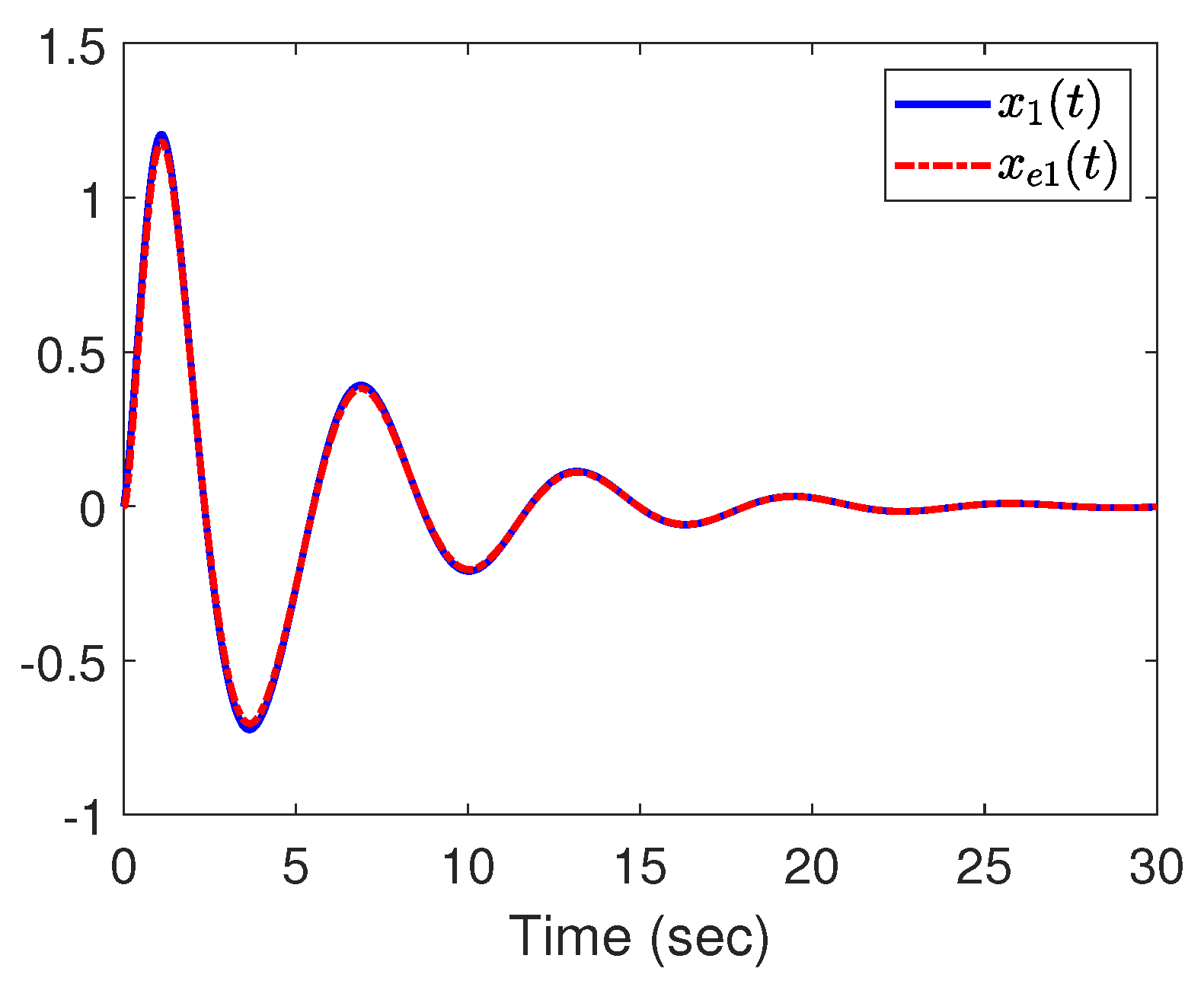
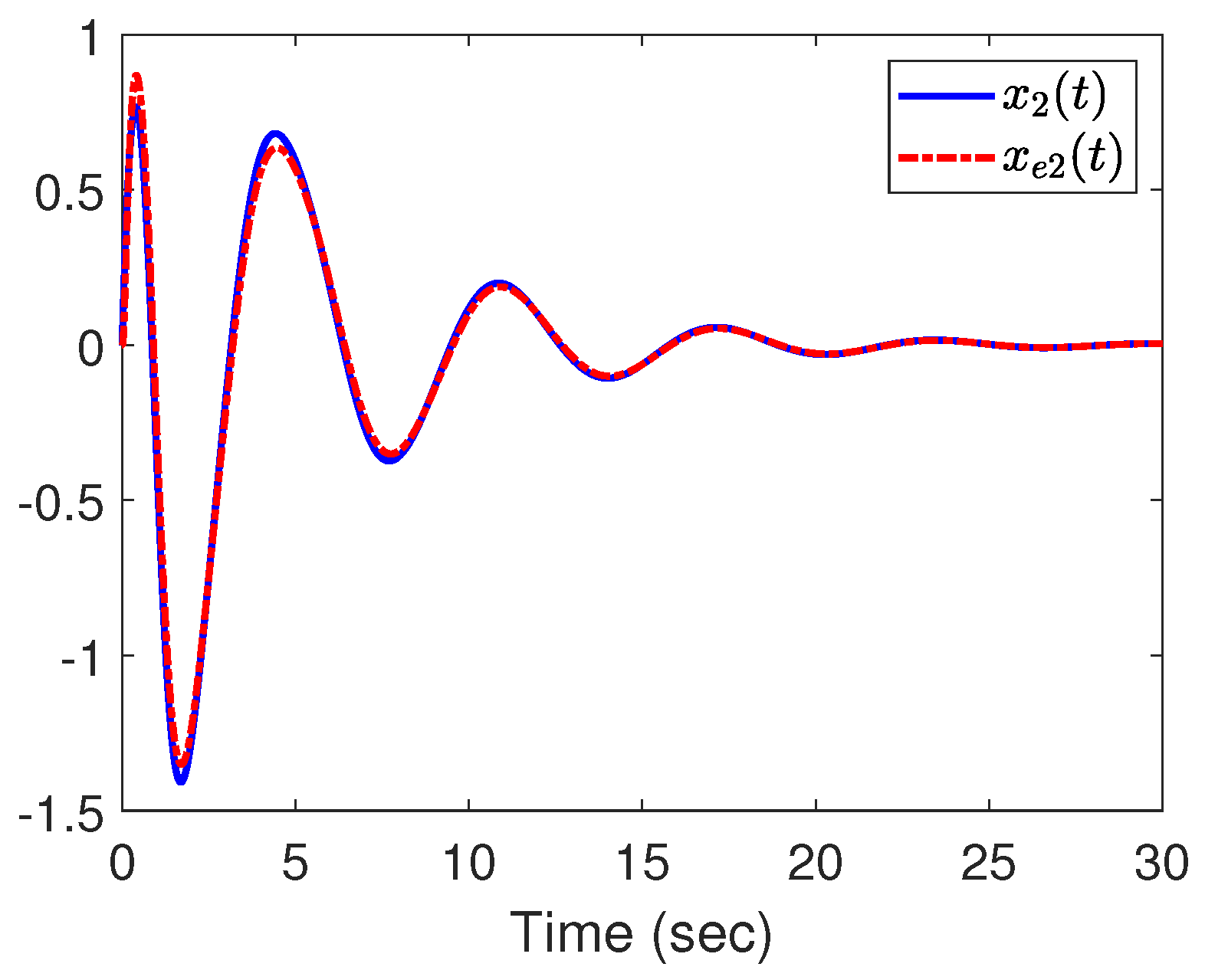
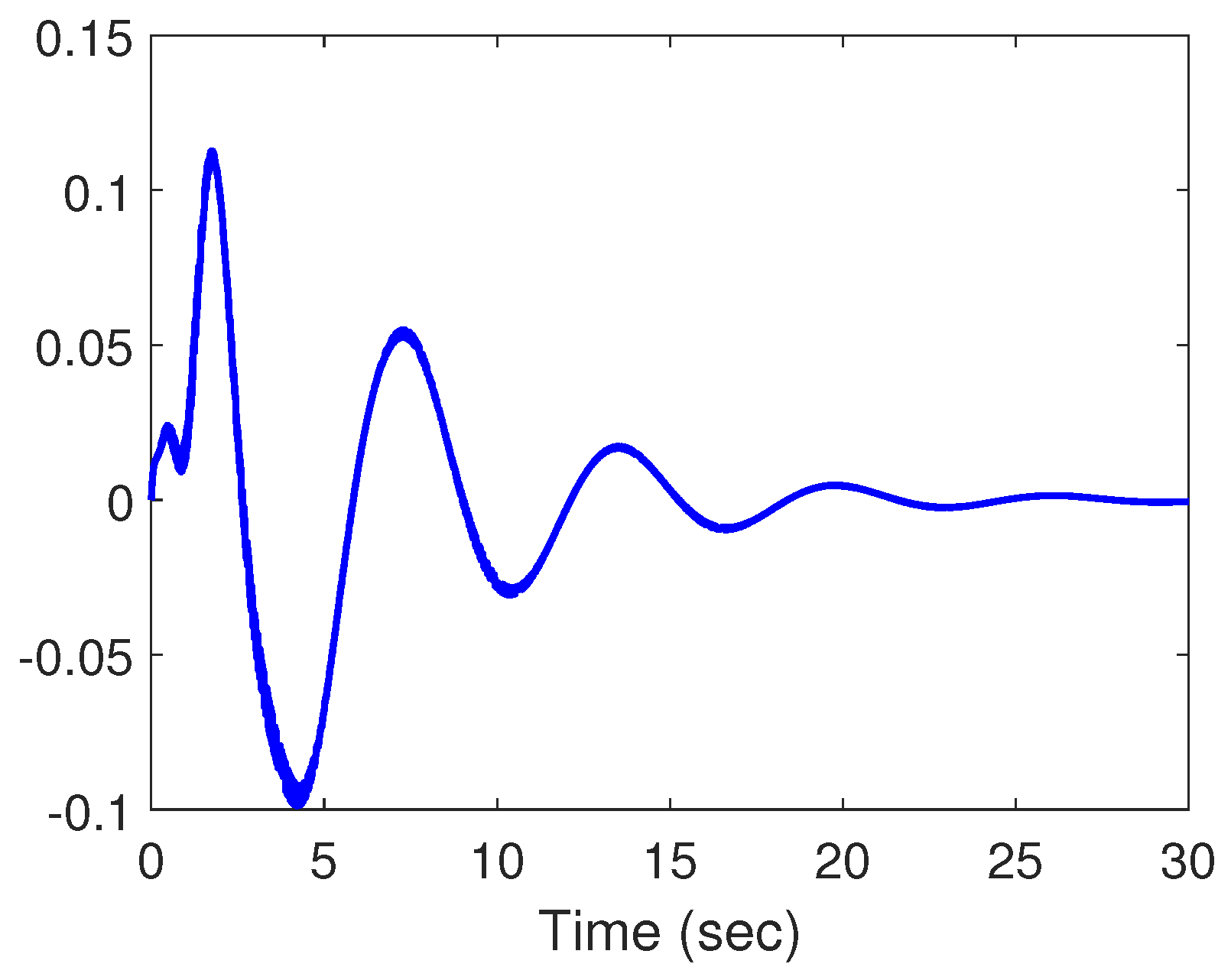
4. Illustrative Example

In this section, the mass-spring mechanical system borrowed from [32] will be utilized to show the effectiveness of the developed co-design strategy. According to the results developed in [32], the equation of motion can be formulated as

$$\begin{array}{c}m\ddot{\chi }+{\mathbb{F}}_f+{\mathbb{F}}_s=u_{\eta }\left(t\right)\hfill \end{array}$$

(39)

where m stands for the mass, $\chi$ represents the displacement from the reference position, $u_{\eta }\left(t\right)$ is the control input. Moreover, ${\mathbb{F}}_f=\omega \dot{\chi }\left(t\right)$ with positive scalar $\omega$ refers to the friction force and ${\mathbb{F}}_s=\delta (1+{\alpha }^2{\chi }^2)$ with scalars $\alpha$ and $\delta$ denotes the restoring force of the spring.

Let us define $x_1\left(t\right)=\chi$, $x_2\left(t\right)=\dot{\chi }$ and select ${\kappa }_1\left(x_1^2\left(t\right)\right)=\frac{x_1^2\left(t\right)-\underline{\chi }}{\overline{\chi }-\underline{\chi }}$, ${\kappa }_2\left(x_1^2\left(t\right)\right)=1-{\kappa }_1\left(x_1^2\left(t\right)\right)$ with $x_1^2\left(t\right)\in \left[\underline{\chi }\overline{\chi }\right]$. Then, the T–S fuzzy model for the nonlinear system in (39) can be represented as:

$$\begin{array}{c}\mathrm{Plant}\mathrm{Rule}1:\mathrm{IF}{x}_1^2\left(t\right)\mathrm{is}\overline{\chi },\mathrm{THEN}\hfill \\ \dot{x}\left(t\right)=A_{1}x\left(t\right)+B_1{u}_{\eta }\left(t\right)\hfill \\ \mathrm{Plant}\mathrm{Rule}2:\mathrm{IF}{x}_1^2\left(t\right)\mathrm{is}\underline{\chi },\mathrm{THEN}\hfill \\ \dot{x}\left(t\right)=A_{2}x\left(t\right)+B_2{u}_{\eta }\left(t\right)\hfill \end{array}$$

(40)

with

$$\begin{array}{c}{A}_1=\left[\begin{array}{cc}0& 1\\ \frac{-\delta (1+{\alpha }^2\overline{\chi })}{m}& \frac{\omega }{m}\end{array}\right],B_1=\left[\begin{array}{c}0\\ \frac{1}{m}\end{array}\right],\hfill \\ A_2=\left[\begin{array}{cc}0& 1\\ \frac{-\delta (1+{\alpha }^2\underline{\chi })}{m}& \frac{\omega }{m}\end{array}\right],B_2=\left[\begin{array}{c}0\\ \frac{1}{m}\end{array}\right].\hfill \end{array}$$

As in [35,39], we assume $m=1$ kg, $\omega =2$ N.m/s, $\delta =5$, $\alpha =0.3$ ${\mathrm{m}}^{-1}$. The corresponding system parameter matrices $D_1$, $D_2$, $C_1$, and $C_2$ are assumed to be

$$\begin{array}{c}{D}_1=D_2=\left[\begin{array}{c}0.1\\ 0.5\end{array}\right],C_1=C_2=\left[10\right].\hfill \end{array}$$

In addition, the parameters for the reference model in (5) are assumed to be

$$\begin{array}{c}{A}_{\xi }=-1,B_{\xi }=0.5,C_{\xi }=1,\hfill \end{array}$$

and the given parameters for the non-fragile observer in (6) and the non-fragile tracking controller in (7) are selected as

$$\begin{array}{c}{X}_{L1}=\left[\begin{array}{c}0.15\\ 0.5\end{array}\right],X_{L2}=\left[\begin{array}{c}0.10\\ 0.7\end{array}\right],Y_L=0.2,\hfill \\ X_{G1}=0.3,X_{G2}=0.2,Y_G=\left[0.30.1\right],\hfill \\ X_{S1}=-0.5,X_{S2}=0.2,Y_S=0.1.\hfill \end{array}$$

By applying Theorem 2 with $M_u=50$, $M_y=100$, $M_{\widehat{x}}=30$, ${\Delta }_u=0.02$, ${\Delta }_y=0.01$, ${\Delta }_{\widehat{x}}=0.05$, ${\beta }_L={\beta }_G={\beta }_S=0.5$, it can be obtained that ${\sigma }_{min}=0.5471$, $f_y=0.0107$, $f_u=0.0203$, $f_{\widehat{x}}=0.0335$, and

$$\begin{array}{c}{L}_1=\left[\begin{array}{c}25.4302\\ 143.5209\end{array}\right],L_2=\left[\begin{array}{c}18.1018\\ 103.3758\end{array}\right],\hfill \\ G_1=[-0.0747-0.0527],S_1=-0.1199,\hfill \\ G_2=[-0.0059-0.0479],S_2=0.1267.\hfill \end{array}$$

To demonstrate the effectiveness of the proposed co-design strategy, we assume that the initial conditions are $x\left(0\right)=x_e\left(0\right)={\left[00\right]}^T$, $\widehat{x}\left(0\right)=0$, the noise input is $\nu \left(t\right)=9cos(t-0.5)exp(-0.2t)$, the uncertain matrices ${\Delta }_L=0.1sin\left(0.5t\right)$, ${\Delta }_G=0.2sin\left(0.5t\right)$, ${\Delta }_S=0.3sin\left(0.5t\right)$, and the bounded reference input is $\xi \left(t\right)=4cos\left(t\right)exp(-0.2t)$. The responses of $x\left(t\right)$ and $x_e\left(t\right)$ are shown in Figure 2 and Figure 3. Figure 4 displays the trajectory of $u\left(t\right)$. The trajectories of $y\left(t\right)$ and $\widehat{y}\left(t\right)$ are given in Figure 5. Figure 6 shows the trajectory of $y_{\epsilon }\left(t\right)$. The ratio of $\sqrt{{\int }_0^{t_r}{y}_{\epsilon }^T\left(t\right)y_{\epsilon }\left(t\right)dt/{\int }_0^{t_r}{\nu }_{\epsilon }^T\left(t\right){\nu }_{\epsilon }\left(t\right)dt}$ is shown in Figure 7. The variations in $j_u\left(t\right)$, $j_y\left(t\right)$, and $j_{\widehat{x}}\left(t\right)$ are displayed in Figure 8, Figure 9, and Figure 10, respectively.

From Figure 2 and Figure 3, it can be seen that the designed non-fragile observer can estimate the unmeasurable state variable of the fuzzy system in (40) effectively. With the observer-based non-fragile tracking controllers shown in Figure 4, Figure 5 and Figure 6 demonstrate that the output $y\left(k\right)$ tracks the reference output $y_{\epsilon }\left(k\right)$ with an acceptable tracking error, as expected. It can be observed from Figure 7 that the ratio of $\sqrt{{\int }_0^{t_r}{y}_{\epsilon }^T\left(t\right)y_{\epsilon }\left(t\right)dt/{\int }_0^{t_r}{\nu }_{\epsilon }^T\left(t\right){\nu }_{\epsilon }\left(t\right)dt}$ tends toward a constant value of 0.0269 below 0.5471, i.e., the prescribed tracking performance can be guaranteed. Moreover, the simulation results in Figure 8, Figure 9 and Figure 10 illustrate that the online adjusting strategies developed in this paper are feasible. Based on the above discussions, it can be concluded that the proposed co-design strategy is effective for the mass-spring mechanical system considered in this paper.

Next, a step-tracking response will be given to further show the effectiveness of the proposed co-design strategy. We assume that $x\left(0\right)={\left[0.50\right]}^T$, $x_e\left(0\right)={\left[00\right]}^T$, $\widehat{x}\left(0\right)=-0.5$,

$$\begin{array}{c}v\left(t\right)=\left\{\begin{array}{cc}3sin\left(0.5t\right),\hfill & 6\le t\le 18\hfill \\ 0,\hfill & \mathrm{otherwise}\hfill \end{array}\right.,\hfill \\ r\left(k\right)=\left\{\begin{array}{cc}-0.85,\hfill & 7\le t\le 12\hfill \\ 0.85,\hfill & 12<t\le 17\hfill \\ 0,\hfill & \mathrm{otherwise}\hfill \end{array}\right..\hfill \end{array}$$

The response of $y\left(t\right)$ and $\widehat{y}\left(t\right)$ in this case is plotted in Figure 11. From Figure 11, it can be seen that the proposed co-design strategy is also effective.

Comparative Explanations: This example shows that the developed co-design strategy can effectively solve the observer-based non-fragile ${\mathcal{H}}_{\infty }$ output feedback tracking control problem for the mass-spring mechanical system in (39) with dynamic quantization and randomly occurring gain variations based on the T–S fuzzy model strategy. In contrast with the existing results, the main advantages of the proposed co-design strategy are summarized as follows:

(1) Compared with the quantized stabilization or ${\mathcal{H}}_{\infty }$ control problem addressed in [2,3,4,5,6,7,8,9,20,21,22,23], the quantized tracking control problem presented here is more difficult and more general. In contrast with the quantized tracking control problem considered in [38,39], the dynamical quantization methodology employed herein is more general. This is mainly because the asymptotical stability of the resulting system can be guaranteed with a finite number of quantization levels. Moreover, the transmission problem of dynamic parameters $j_z\left(t\right)$ ($z=u,y,\widehat{x}$) was considered in this paper, and Figure 8, Figure 9 and Figure 10 show that the adjustment of the dynamic parameters $j_z\left(t\right)$ can be realized based on the online adjusting strategies developed in (15) combined with Remark 3. This implies that we no longer need to assume that the same dynamic parameters $j_z\left(t\right)$ are obtained on both sides of the communication network according to the quantized signal $z_{\eta }\left(t\right)$ ($z=u,y,\widehat{x}$), as in [9,27,40].

(2) The observer and the tracking controller employed are non-fragile, with randomly occurring gain variations rather than the fragile ones considered in [32,33,35]. The developed observer-based tracking control strategy allows for the control inputs of the observer and the plant to be different, which implies that the restrictive assumption in [35], i.e., the control inputs of the observer and the plant are the same, has been avoided. In contrast with the singular value decomposition approach used in [35], the descriptor representation approach developed in this paper is more general because it can effectively avoid the constraint on the system output matrix C. Moreover, this example illustrates that the desired non-fragile observer and non-fragile tracking controller can be obtained simultaneously by solving the linear matrix inequalities in (31)–(34) rather than the two-step design strategy developed in [32,33].

5. Conclusions

In this paper, based on the T–S fuzzy model strategy, the observer-based non-fragile ${\mathcal{H}}_{\infty }$ output feedback tracking control problem was studied for nonlinear networked systems with dynamic quantization and randomly occurring gain variations. The dynamical quantization methodology was employed to enhance the efficiency in the utilization of the limited communication resources. By utilizing the descriptor representation strategy combined with the S-procedure, a co-design strategy for the desired dynamic quantizers and observer-based non-fragile output feedback tracking controller was formulated in terms of linear matrix inequalities. Moreover, a simulation example was proposed to demonstrate the effectiveness of the proposed co-design method. Next, the non-fragile output feedback tracking control problem will be investigated for the switched nonlinear systems considered in [46] or uncertain planar nonlinear systems addressed in [47].

References

1. Zhang, L.; Gao, H.; Kaynak, O. Network-induced constraints in networked control systems—A survey. IEEE Trans. Ind. Inf. 2013, 9, 142–149. [Google Scholar] [CrossRef]
2. Su, L.; Chesi, G. Robust stability of uncertain linear systems with input and output quantization and packet loss. Automatica 2018, 87, 267–273. [Google Scholar] [CrossRef]
3. Gao, H.; Chen, T. A new approach to quantized feedback control systems. Automatica 2008, 44, 534–542. [Google Scholar] [CrossRef]
4. Coutinho, D.F.; Fu, M.; de Souza, C.E. Input and output quantized feedback linear systems. IEEE Trans. Autom. Control 2010, 55, 761–766. [Google Scholar] [CrossRef]
5. Liberzon, D. Hybrid feedback stabilization of systems with quantized signals. Automatica 2003, 39, 1543–1554. [Google Scholar] [CrossRef]
6. Che, W.W.; Yang, G.H. State feedback H control for quantized discrete-time systems. Asian J. Contr. 2008, 10, 718–723. [Google Scholar] [CrossRef]
7. Zheng, B.C.; Yu, X.; Xue, Y. Quantized feedback sliding-mode control: An event-triggered approach. Automatica 2018, 91, 126–135. [Google Scholar] [CrossRef]
8. Niu, Y.; Ho, D.W.C. Control strategy with adaptive quantizer’s parameters under digital communication channels. Automatica 2014, 50, 2665–2671. [Google Scholar] [CrossRef]
9. Chang, X.H.; Xiong, J.; Li, Z.M.; Park, J.H. Quantized static output feedback control for discrete-time systems. IEEE Trans. Ind. Inf. 2018, 14, 3426–3435. [Google Scholar] [CrossRef]
10. Tanaka, K.; Wang, H.O. Fuzzy Control Systems Design and Analysis: A Linear Matrix Inequality Approach; Wiley: New York, NY, USA, 2001. [Google Scholar]
11. Takagi, T.; Sugeno, M. Fuzzy identification of systems and its applications to modeling and control. IEEE Trans. Syst. Man Cybern. 1985, 15, 116–132. [Google Scholar] [CrossRef]
12. Zhang, J.; Shi, P.; Qiu, J.; Nguang, S.K. A novel observer-based output feedback controller design for discrete-time fuzzy systems. IEEE Trans. Fuzzy Syst. 2015, 23, 223–229. [Google Scholar] [CrossRef]
13. Chang, X.H.; Yang, G.H. Nonfragile H filter design for T–S fuzzy systems in standard form. IEEE Trans. Ind. Electron. 2014, 61, 3448–3458. [Google Scholar] [CrossRef]
14. Dong, J.; Yang, G.H. Observer-based output feedback control for discrete-time T–S fuzzy systems with partly immeasurable premise variables. IEEE Trans. Syst. Man Cybern. Syst. 2017, 47, 98–110. [Google Scholar] [CrossRef]
15. Chang, X.H.; Yang, G.H. A descriptor representation approach to observer-based H control synthesis for discrete-time fuzzy systems. Fuzzy Sets Syst. 2011, 185, 38–51. [Google Scholar] [CrossRef]
16. Liu, Y.; Guo, B.Z.; Park, J.H. Non-fragile H filtering for delayed Takagi-Sugeno fuzzy systems with randomly occurring gain variations. Fuzzy Sets Syst. 2017, 316, 99–116. [Google Scholar] [CrossRef]
17. Zhang, H.; Yang, D.; Chai, T. Guaranteed cost networked control for T–S fuzzy systems with time delays. IEEE Trans. Syst. Man Cybern. C 2007, 37, 160–172. [Google Scholar] [CrossRef]
18. Yao, H.; Gao, F. Design of observer and dynamic output feedback control for fuzzy networked systems. Mathematics 2022, 11, 148. [Google Scholar] [CrossRef]
19. Peng, C.; Yang, T.C. Communication-delay-distribution-dependent networked control for a class of T–S fuzzy systems. IEEE Trans. Fuzzy Syst. 2010, 18, 326–335. [Google Scholar] [CrossRef]
20. Zheng, Q.; Xu, S.; Zhang, Z. Nonfragile H control for uncertain Takagi-Sugeno fuzzy systems under digital communication channels and its application. IEEE Trans. Syst. Man Cybern. Syst. 2022, 52, 3638–3647. [Google Scholar] [CrossRef]
21. Shen, H.; Men, Y.; Wu, Z.G.; Cao, J.; Lu, G. Network-based quantized control for fuzzy singularly perturbed semi-Markov jump systems and its application. IEEE Trans. Circuits Syst. I Reg. Papers 2019, 66, 1130–1140. [Google Scholar] [CrossRef]
22. Qiu, J.; Feng, G.; Gao, H. Observer-based piecewise affine output feedback controller synthesis of continuous-time T–S fuzzy affine dynamic systems using quantized measurements. IEEE Trans. Fuzzy Syst. 2012, 20, 1046–1062. [Google Scholar]
23. Chang, X.H.; Yang, C.; Xiong, J. Quantized fuzzy output feedback H control for nonlinear systems with adjustment of dynamic parameters. IEEE Trans. Syst. Man Cybern. Syst. 2019, 49, 2005–2015. [Google Scholar] [CrossRef]
24. Zheng, Q.; Xu, S.; Du, B. Quantized guaranteed cost output feedback control for nonlinear networked control systems and its applications. IEEE Trans. Fuzzy Syst. 2022, 30, 2402–2411. [Google Scholar] [CrossRef]
25. Pan, T.T.; Chang, X.H.; Liu, Y. Robust fuzzy feedback control for nonlinear systems with input quantization. IEEE Trans. Fuzzy Syst. 2022, 30, 4905–4914. [Google Scholar] [CrossRef]
26. Chang, X.H.; Jin, X. Observer-based fuzzy feedback control for nonlinear systems subject to transmission signal quantization. Appl. Math. Comput. 2022, 414, 126657. [Google Scholar] [CrossRef]
27. Chang, X.H.; Li, Z.M.; Park, J.H. Fuzzy generalized H2 filtering for nonlinear discrete-time systems with measurement quantization. IEEE Trans. Syst. Man Cybern. Syst. 2018, 48, 2419–2430. [Google Scholar] [CrossRef]
28. Li, Z.M.; Xiong, J. Event-triggered fuzzy filtering for nonlinear networked systems with dynamic quantization and stochastic cyber attacks. ISA Trans. 2022, 121, 53–62. [Google Scholar] [CrossRef]
29. Gao, H.; Chen, T. Network-based H output tracking control. IEEE Trans. Autom. Control 2008, 53, 655–667. [Google Scholar] [CrossRef]
30. Peng, C.; Song, Y.; Xie, X.P.; Zhao, M.; Fei, M.R. Event-triggered output tracking control for wireless networked control systems with communication delays and data dropouts. IET Control Theory Appl. 2016, 10, 2195–2203. [Google Scholar] [CrossRef]
31. Yan, H.; Hu, C.; Zhang, H.; Karimi, H.R.; Jiang, X.; Liu, M. H output tracking control for networked systems with adaptively adjusted event-triggered scheme. IEEE Trans. Syst. Man Cybern. Syst. 2019, 49, 2050–2058. [Google Scholar] [CrossRef]
32. Lian, K.Y.; Liou, J.J. Output tracking control for fuzzy systems via output feedback design. IEEE Trans. Fuzzy Syst. 2006, 14, 628–639. [Google Scholar] [CrossRef]
33. Lin, C.; Wang, Q.G.; Lee, T.H. H output tracking control for nonlinear systems via T–S fuzzy model approach. IEEE Trans. Syst. Man Cybern. B Cybern. 2006, 36, 450–457. [Google Scholar]
34. Tseng, C.S.; Chen, B.S.; Uang, H.J. Fuzzy tracking control design for nonlinear dynamic systems via T–S fuzzy model. IEEE Trans. Fuzzy Syst. 2001, 9, 381–392. [Google Scholar] [CrossRef] [Green Version]
35. Li, H.; Wu, C.; Jing, X.; Wu, L. Fuzzy tracking control for nonlinear networked systems. IEEE Trans. Cybern. 2017, 47, 2020–2031. [Google Scholar] [CrossRef]
36. Zhang, D.; Han, Q.L.; Jia, X. Network-based output tracking control for a class of T–S fuzzy systems that can not be stabilized by nondelayed output feedback controllers. IEEE Trans. Cybern. 2015, 45, 1511–1524. [Google Scholar] [CrossRef]
37. Zhang, D.; Han, Q.L.; Jia, X. Network-based output tracking control for T–S fuzzy systems using an event-triggered communication scheme. Fuzzy Sets Syst. 2015, 273, 26–48. [Google Scholar] [CrossRef]
38. Li, Z.M.; Park, J.H. Dissipative fuzzy tracking control for nonlinear networked systems with quantization. IEEE Trans. Syst. Man Cybern. Syst. 2020, 50, 5130–5141. [Google Scholar] [CrossRef]
39. Li, Z.M.; Chang, X.H.; Park, J.H. Quantized static output feedback fuzzy tracking control for discrete-time nonlinear networked systems with asynchronous event-triggered constraints. IEEE Trans. Syst. Man Cybern. Syst. 2021, 51, 3820–3831. [Google Scholar] [CrossRef]
40. Li, Z.M.; Chang, X.H.; Xiong, J. Event-based fuzzy tracking control for nonlinear networked systems subject to dynamic quantization. IEEE Trans. Fuzzy Syst. 2022. in press. Available online: https://ieeexplore.ieee.org/abstract/document/9839441 (accessed on 25 July 2022).
41. Wu, L.; Yang, X.; Li, F. Nonfragile output tracking control of hypersonic air-breathing vehicles with an LPV model. IEEE/ASME Trans. Mechatron. 2013, 18, 1280–1288. [Google Scholar] [CrossRef]
42. Keel, L.H.; Bhattacharyya, S.P. Robust, fragile, or optimal? IEEE Trans. Autom. Control 1997, 42, 1098–1105. [Google Scholar] [CrossRef]
43. Wang, J.; Wu, J.; Cao, J.; Chadli, M.; Shen, H. Nonfragile output feedback tracking control for Markov jump fuzzy systems based on integral reinforcement learning scheme. IEEE Trans. Cybern. 2022. in press. Available online: https://ieeexplore.ieee.org/abstract/document/9911218 (accessed on 4 October 2022).
44. Han, T.J.; Kim, H.S. Disturbance observer-based nonfragile fuzzy tracking control of a spacecraft. Adv. Space Res. 2022. in press. Available online: https://www.sciencedirect.com/science/article/abs/pii/S0273117722010754 (accessed on 25 November 2022).
45. Ghorbel, C.; Benhadj Braiek, N. Nonfragile H tracking control strategies for classes of linear and bilinear uncertain Takagi-Sugeno fuzzy systems. Trans. Inst. Meas. Control 2022, 44, 2166–2176. [Google Scholar] [CrossRef]
46. Gao, F.; Wu, Y.; Zhang, Z. Global fixed-time stabilization of switched nonlinear systems: A time-varying scaling transformation approach. IEEE Trans. Circuits Syst. II Exp. Briefs 2019, 66, 1890–1894. [Google Scholar] [CrossRef]
47. Gao, F.; Chen, C.C.; Huang, J.; Wu, Y. Prescribed-time stabilization of uncertain planar nonlinear systems with output constraints. IEEE Trans. Circuits Syst. II Exp. Briefs 2022, 69, 2887–2891. [Google Scholar] [CrossRef]
Figure 1. The block diagram of nonlinear networked systems.
Mathematics 11 01116 g001
Figure 2. The trajectories of  x 1 ( t ) and  x e 1 ( t ) .
Mathematics 11 01116 g002
Figure 3. The trajectories of  x 2 ( t ) and  x e 2 ( t ) .
Mathematics 11 01116 g003
Figure 4. The trajectory of the control input  u ( t ) .
Mathematics 11 01116 g004
Figure 5. The trajectories of  y ( t ) and  y ^ ( t ) .
Mathematics 11 01116 g005
Figure 6. The trajectory  y ε ( t ) .
Mathematics 11 01116 g006
Figure 7. The ratio of  0 t r y ε T ( t ) y ε ( t ) d t / 0 t r ν ε T ( t ) ν ε ( t ) d t .
Mathematics 11 01116 g007
Figure 8. The trajectory of  j u ( t ) .
Mathematics 11 01116 g008
Figure 9. The trajectory of  j y ( t ) .
Mathematics 11 01116 g009
Figure 10. The trajectory of  j x ^ ( t ) .
Mathematics 11 01116 g010
Figure 11. The trajectories of  y ( t ) and  y ^ ( t ) .
Mathematics 11 01116 g011
Disclaimer/Publisher’s Note: The statements, opinions and data contained in all publications are solely those of the individual author(s) and contributor(s) and not of MDPI and/or the editor(s). MDPI and/or the editor(s) disclaim responsibility for any injury to people or property resulting from any ideas, methods, instructions or products referred to in the content.