Article

Data-Driven pH Model in Raceway Reactors for Freshwater and Wastewater Cultures

by
Pablo Otálora
1,*,†,
José Luis Guzmán
1,†,
Manuel Berenguel
1,† and
Francisco Gabriel Acién
2,†
1
Department of Informatics, University of Almería, ceiA3, CIESOL, Ctra. Sacramento s/n, 04120 Almería, Spain
2
Department of Chemical Engineering, University of Almería, ceiA3, CIESOL, Ctra. Sacramento s/n, 04120 Almería, Spain
*
Author to whom correspondence should be addressed.
These authors contributed equally to this work.
Mathematics 2023, 11(7), 1614; https://doi.org/10.3390/math11071614
Submission received: 24 January 2023 / Revised: 13 March 2023 / Accepted: 23 March 2023 / Published: 27 March 2023

Abstract

:
The industrial production of microalgae is a process as sustainable as it is interesting in terms of its diverse applications, especially for wastewater treatment. Its optimization requires an exhaustive knowledge of the system, which is commonly achieved through models that describe its dynamics. Although not widely used in this field, artificial neural networks are presented as an appropriate technique to develop this type of model, having the ability to adapt to complex and nonlinear problems solely from the process data. In this work, neural network models have been developed to characterize the pH dynamics in two different raceway reactors, one with freshwater and the other with wastewater. The models are able to predict pH profiles with a prediction horizon of up to eleven hours and only using available measurable process data, such as medimum level, CO 2 injection, and solar radiation. The results demonstrate the potential of artificial neural networks in the modeling of continuous dynamic systems in the field of industry, obtaining accurate, fast-running models that can adapt to different circumstances. Moreover, these models open the field to the design of data-driven model-based control algorithms to account for the nonlinear dynamics of this biological system.

1. Introduction

The sustainability of our current lifestyle is one of the leading issues in recent years. Society is looking for measures to guarantee the supply of essential resources such as food, water and energy while reducing environmental impact and maximizing economic yield. As a result, new technologies are emerging as an answer to the traditional alternatives to address these problems. One of these is the industrial production of microalgae [1].
The industrial production of microalgae is a technology with growing impact in recent decades. Microalgae are photosynthetic microorganisms with the ability to grow and reproduce without the need for freshwater or fertile soil [2]. They have high growth rates and are tolerant to wide temperature ranges, and the composition of their biomass is very interesting for applications in the fields of human or animal nutrition, cosmetics, production of fertilizers or biostimulants, among others [3]. Their ability to grow also makes them a potential source of biofuel [4]. However, their main application and the field in which they are particularly promising is in wastewater treatment [5].
Microalgae require at least three elements for their development: water, light and nutrients [6,7]. Water is always obtained in excess, since microalgae are normally grown in an aqueous medium. Light can be obtained in different ways depending on the mode of production. Microalgae can circulate through forced conduits, with no contact with the outside, preventing the insertion of external contaminants and being able to tightly control the conditions in which they are found. These conduits are known as tubular photobioreactors, and in these, the light source can be artificial (when used indoors) or natural from the sunlight (when used outdoors). The alternative to to those is the open reactors, called raceways, which always use the sun as a light source [8]. These reactors are large open ponds in which the medium flows with the microalgae, being exposed to external contaminants and with harder to control conditions. However, this mode is the easiest to scale up and the most financially viable, making it the most extended at the industrial level, limiting the use of tubular photobioreactors to the production of high-value products that must guarantee their purity [9]. This paper will address raceway photobioreactors.
In terms of nutrients, the three most important for culture growth are phosphorus, nitrogen and carbon. The first two can be supplied externally according to the needs of the culture; alternatively, wastewater can be used as a medium, with phosphorus and nitrogen being two of the most common and dangerous nutrients in these, which can cause environmental problems such as eutrophication (excessive growth of algae and aquatic plants that deplete oxygen) in receiving water bodies. Hence, nutrients are usually available in excess, guaranteeing microalgae supply, at the same time as wastewater treatment is performed. Carbon is provided in the form of CO 2 , either pure or from other industrial activity, helping to mitigate its environmental impact while simultaneously controlling culture conditions [10].
However, for microalgae production to be competitive, it is crucial to maximize their productivity. Productivity is not only dependent on the availability of light, water and nutrients but also on the available radiation and the pH, dissolved oxygen (DO) and temperature of the medium [11]. Among these variables, radiation is the only one that is not usually regulated in raceway photobioreactors [12], as it depends on the environmental conditions of the day, although it is important to be considered when selecting the location of the system [13]. DO presents a threshold value at which productivity is drastically reduced, and so the control problem is centered on maintaining it below this threshold, regardless of its value as long as this condition is satisfied. This is accomplished through air injection [14], which increases agitation and mixing of the water, leading to an increase in the rate of oxygen transfer from the water to the air, thus reducing this value. Temperature is not usually considered a control objective, although it has an influence on productivity, maximizing it when it is around a specific value, depending on the species cultivated. It can be controlled by modifying the culture depth [15,16].
The pH is often the most important variable in the control problem. Analogous to temperature, when this variable is close to its optimum value, its influence on productivity is positive, while moving away from this value reduces the productivity of the process, thus making its control a critical issue. Its value can be controlled by injecting CO 2 , so that the carbon supply and pH control problem can be solved simultaneously [17].
Nevertheless, the biological nature of the system makes the problem far from trivial. The pH dynamics are highly nonlinear and very changing not only between seasons but also over the duration of a day due to the variable capability of the microalgae to photosynthesize. This makes it extremely difficult to characterize the process, being a critical issue when developing control strategies [18,19].
Traditional models developed for this system can be sorted into two types. On one side are the first principles-based models, oriented to a more chemical approach and focused on reflecting the interactions between the different elements of the system. These models provide a high degree of understanding of the process, but they are not very useful for achieving the control objectives given their high complexity and long execution time [20]. The alternative to these models is low-order experimental models, which are simple and quick to obtain but very limited in terms of their representation of the system, quickly becoming obsolete due to the aforementioned variability [21,22]. This means that they must be constantly recalibrated, which is not always possible.
Regarding the state of art, in [23], a dynamic model for the pH in tubular photobioreactors was developed based on fluid-dynamics, mass tranfer and biological phenomena. The model is accurate and useful for many purposes, but it is limited to closed photobioreactors. Fernández et al. [24] present a similar model, based on first principles, for a raceway reactor calibrated and validated with real data. The model is useful for analyzing the system’s productivity, but its running time is relatively long, and its periodic recalibration is mandatory. Rodríguez-Miranda et al. [25] developed a temperature model for raceway reactors, allowing researchers to model and study this variable, which is crucial to the productivity of the system. In [26], a first-principle-based dynamic model for pH prediction was presented for a torus photobioreactor and validated with experimental data, but it is only valid for this type of reactor. On the other hand, more control-oriented works favor simpler and more experimental models. Pawlowski et al. [27] present an event-based pH control based on Global Predictive Control (GPC) using an experimental first-order lineal model. Rodríguez-Miranda et al. [28] developed diurnal and nocturnal pH controllers oriented to the different dynamics of each period, all of them based on first-order models.
Machine learning techniques, and more specifically artificial neural networks (ANN), are experiencing a notable increase in popularity in recent years as an alternative to these models due to the increase in the computational capacity of computers as well as the sheer volume of data available [29]. Data acquisition and processing is an increasingly demanded task in all fields due to these types of technique, which are characterized by their ability to adapt to a wide variety of problems based solely on the data without the need to be explicitly programmed for it. They have the capacity to infer patterns in the data beyond human comprehension, being especially useful in image or text processing tasks, speech recognition, and recommendation management.
However, these techniques still have not found much use in the field of dynamic systems modeling, and they have even less use in the field of microalgae production, despite being presented as an excellent option in theory. The models obtained, despite not providing any understanding of the system, as they behave as black-box models, are very fast running, easy to adapt to new data and capable of incorporating the nonlinearities of the system [30]. This makes them a very interesting option for sensor error detection tasks or as the core of Model Predictive Control (MPC) strategies [31,32].
In the specific field of microalgae production, these techniques have found the most use in culture classification. Correa et al. [33] present a neural-network based models for microalgae classification able to distinguish between 19 different classes. Otálora et al. [34] developed a neural network model, which was validated with pure and mixed samples. Regarding the system dynamics, [35] presents a neural network dynamic model for the pH for a raceway reactor with promising results, but it is only valid for freshwater reactors. Caparroz et al. [36] combined first-order models with regression trees in order to keep an easy and transparent formulation combined with the nonlinearity provided from the machine learning technique.
The aim of this work is to develop two neural network models for pH prediction in freshwater and wastewater raceway photobioreactors to analyze the viability of using this data-driven approach for modeling purposes in this kind of plants. The goal of the model is to be able to estimate the pH profile over several hours of a day given a set of predictable or controllable system variables. The model will be trained and validated with real raceway reactor data. The results justify the use of this type of technique in the field of microalgae production and dynamic systems modeling, achieving accurate pH forecasts with prediction horizons of up to 11 h. The proposed models provide relevant potential for the development of model-based control algorithms for this type of process.
The paper is structured as follows: Section 2 describes the modeled system as well as the techniques used and the toolboxes employed. Section 3 details the complete development of the models from data acquisition and processing to training and validation. Finally, Section 4 presents the implications of the research as well as potential future lines of work, and Section 5 states the main conclusions drawn during the development of the work.

2. Materials and Methods

2.1. Modelled Photobioreactors

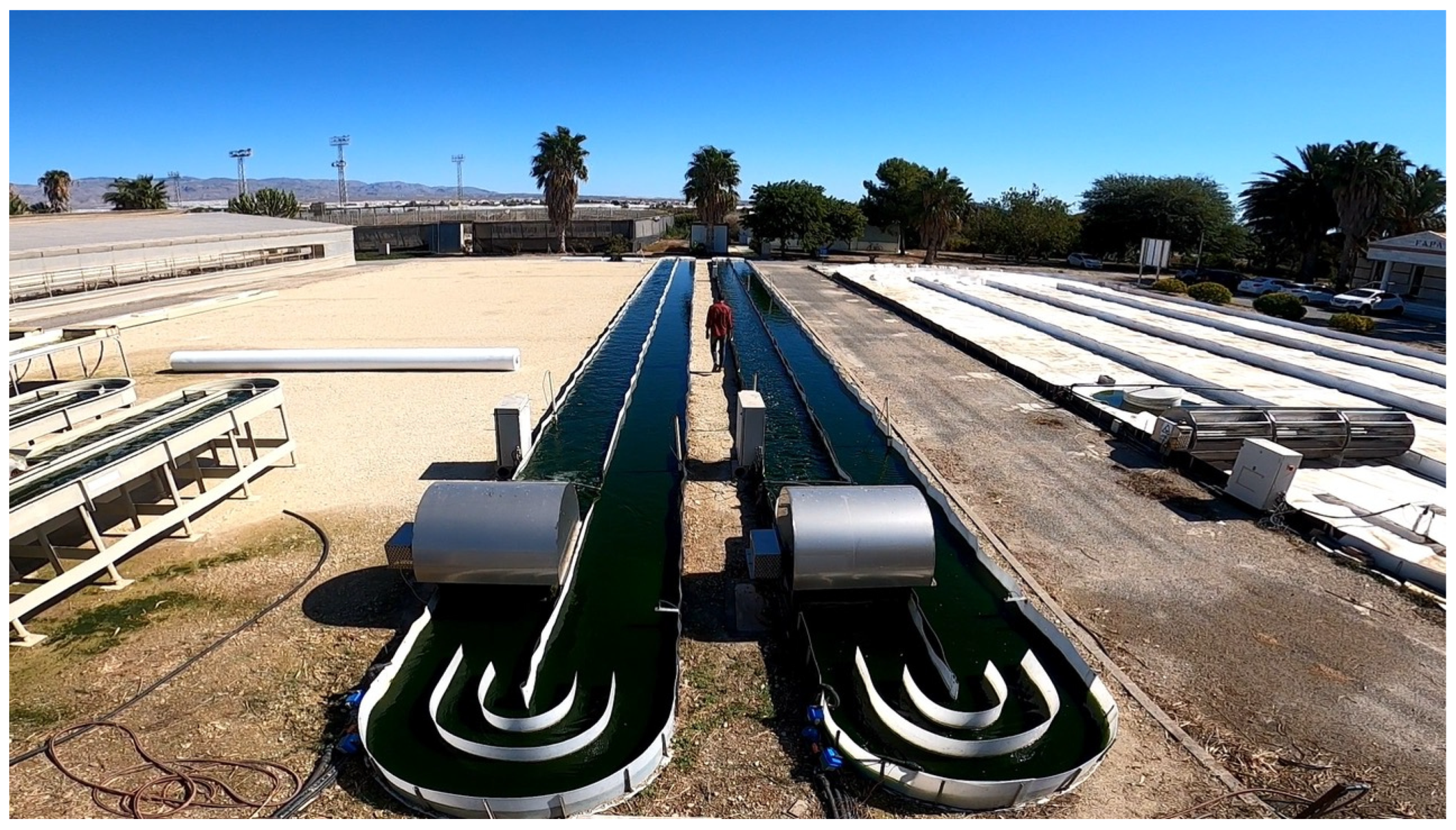
The models obtained in this work correspond to two raceway photobioreactors located at the IFAPA center of the University of Almería (36°50′ N, 2°24′ W), as shown in Figure 1. Both reactors have a similar configuration, consisting of two 40 m long, 1 m wide, and 0.3 m deep channels, although the typical culture height is 15 cm. The channels are joined at their ends by 180 o bends, constituting a total surface of 80 m 2 per reactor. Both feature a paddle wheel driven by an electric motor, which makes the water flow through the entire reactor at a speed of approximately 0.23 m/s. A 1 m deep sump is located 1.8 m away from the paddle wheel in the flow direction through which the injection of CO 2 and air takes place, which is used for pH and DO control, respectively. The main difference between the two reactors is in the medium in which the microalgae are found. The first reactor uses freshwater as its medium with the following composition: 0.9 g/L NaNO 3 , 0.14 g/L KH 2 PO 4 , 0.18 g/L mgSO 4 and 0.03 g/L Kerantol. The second reactor uses wastewater obtained directly from the University of Almería or from a wastewater treatment plant located in Almería.
The microalgae strain cultivated in both reactors is from the species Scenedesmus almeriensis (CCAP 276/24). This is characterized by its high growth rate (0.08 h 1 ) as well as its tolerance to wide condition ranges. They are able to tolerate pH from 3 to 10, its optimum value being 8, as well as temperatures between 12 and 46 °C, the optimum value being 27 °C, which makes it ideal for its production in an area such as Almería. For this reason, it is one of the most used species for cultivation in open reactors and wastewater treatment. It also serves as a source of lutein in the field of human nutrition [37].
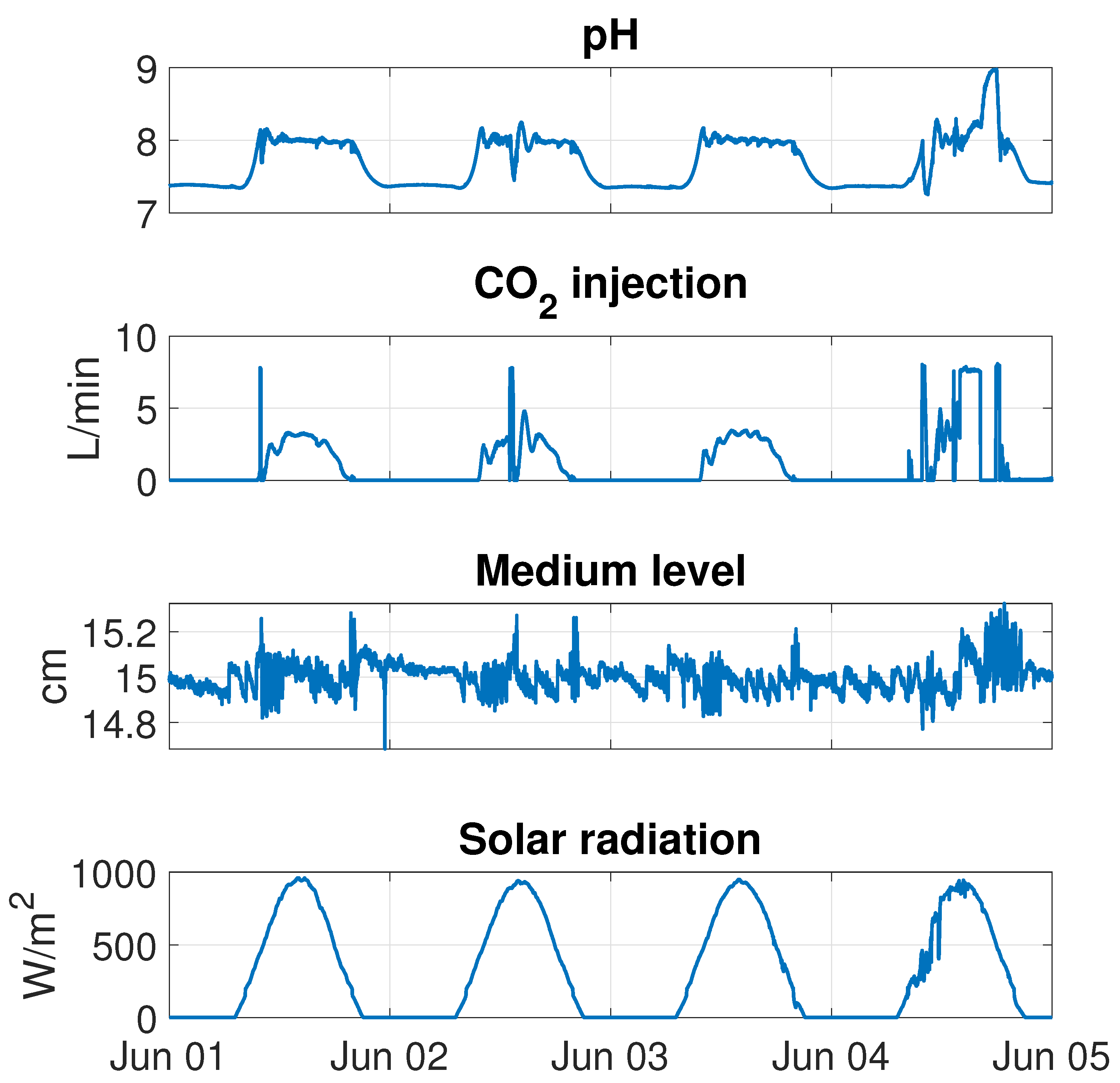
The system is fully sensorized, recording pH, DO and water temperature measurements at two different points: the sump where the injection takes place and the farthest point from it, which is considered the most unfavorable and most challenging to control, the latter being the one usually considered in the control problem. The system also has flowmeters that register the air and CO 2 flow rates injected, a water level sensor, and sensors for environmental variables such as ambient temperature, relative humidity and solar radiation: all of this with a sampling time of one second. The sensors used are shown in Table 1.

2.2. Artificial Neural Networks

Machine learning algorithms are a set of modeling techniques that have the particularity of not being explicitly programmed to solve a problem but instead have the ability to learn from the data provided during their training to learn and adapt to it. There are many machine learning algorithms, and one of the most popular in recent years is artificial neural networks (ANNs).
ANNs owe their name to their resemblance to biological neural networks, since they consist of a set of nodes interconnected with each other in a similar way. Any ANN model has one or more input variables, known as predictors, and one or more output variables, known as predictions. The model is organized in layers; each layer is composed of nodes. Each node of a layer receives as inputs the outputs of the nodes of the previous layer, operates with these, and calculates its own output, which will then be used as input for the nodes of the subsequent layer. The nodes of the first layer receive as inputs the predictors of the model, and those of the last layer return as output the model predictions.
The way nodes operate is different depending on the type of layer they are in. The most typical form is that expressed in Equation (1), where y corresponds to the output of a particular node, x n corresponds to each of its k inputs, which at the same time are the outputs of the nodes of the previous layer, W n corresponds to the weights assigned to each input, b corresponds to the node’s bias and ϕ corresponds to its activation function, which is typically nonlinear. If this activation function was linear, the relationship between inputs and outputs of this layer would also be so, which is the reason why this nonlinear feature is important to grant such behavior to the model.
y = ϕ n = 1 k W n · x n + b
Thus, the model is configured by four fundamental elements: the number of layers, which is in charge of giving it depth and complexity, the number of nodes in each layer, which is related to the model’s capacity to generalize or adapt to more specific situations, the activation function of each layer, and the weights of each node, W n and b. The first three elements are considered before the model development and constitute its structure. Their selection must take into account the type and complexity of the problem as well as the data used and the desired characteristics of the model. On the other hand, the weights of the nodes are calculated during the training process. In this process, a set of input and output data is taken, known as the training dataset, and the algorithm iteratively calculates the weights of each node to minimize the difference between the model predictions and the real ouput data.
The development process of an ANN model therefore consists of three steps. First, the predictors and variables to be predicted must be selected and the relevant analyses must be performed. From these, the data set is prepared with the necessary processing. Since these are data-based models, it is critical for the data to be realistic, adequate and sufficient; otherwise, the model will not be acceptable. The second step is the selection of the model structure. This involves the number of layers, the type of each layer, their activation functions, and the connections between layers. Many of these parameters are commonly obtained iteratively, since there is no way to know beforehand the optimal structure to solve a problem. Finally, the third and last step is the training of the selected model with the prepared data. This training will be dictated by a series of hyperparameters related to training duration, data splitting, learning rate or the optimization function.
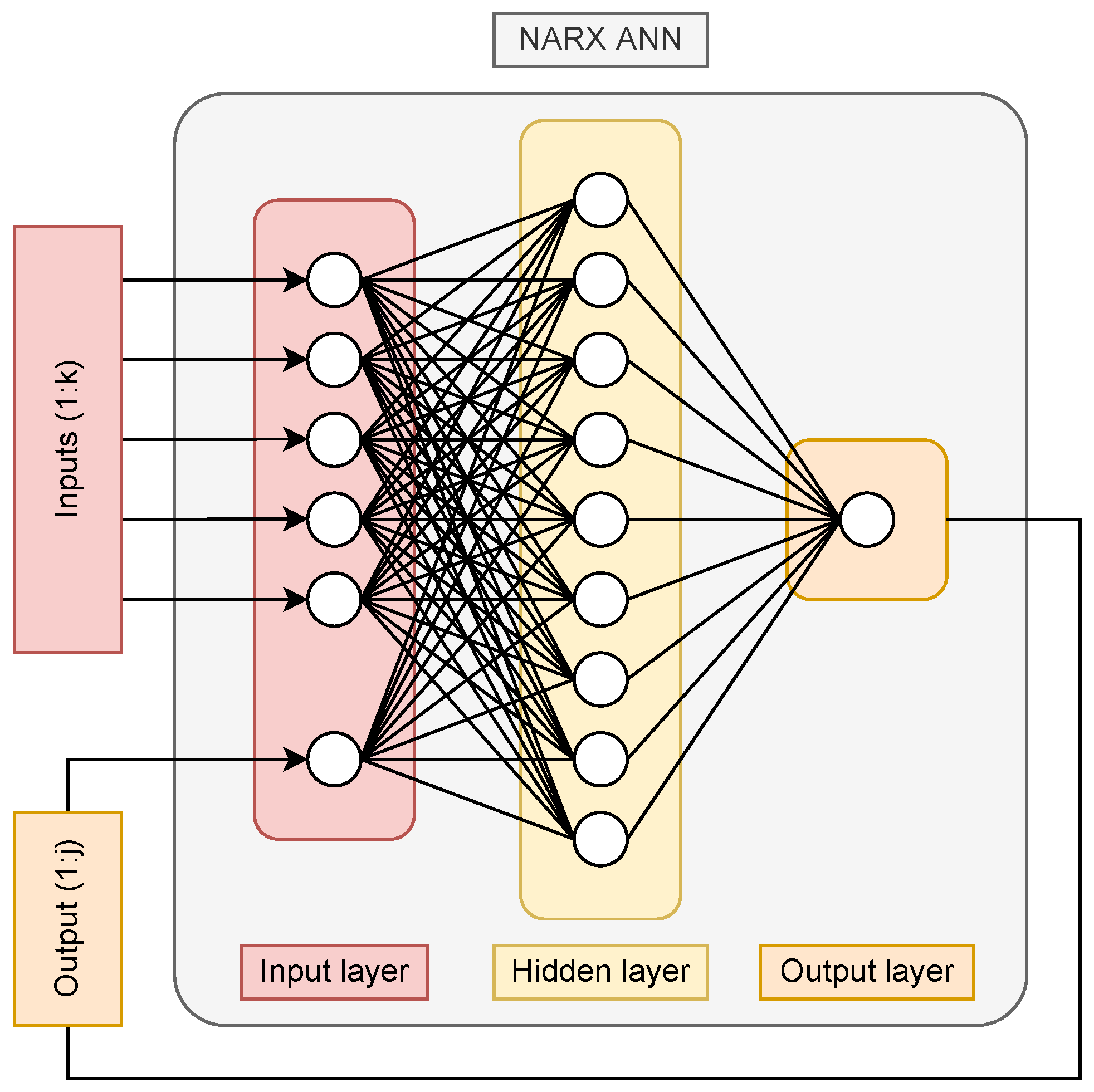
Classic ANNs are particularly appropriate for solving static problems, where the model does not need to reflect time dependence. However, for the pH modeling problem addressed, the system has a clearly dynamic character, making it necessary to adopt an ANN structure able to capture such behavior. The most common models for this are Long Short-Term Memory (LSTM), convolutional, or Nonlinear AutoRegressive with eXogenous inputs (NARX) ANNs. Among these, NARX are the simplest as well as the ones that offer a description most similar to a classical dynamic model [38].
The foundation of NARX-type models is the use of the n prior values of each predictor to predict the next value of the output variable. The model also uses the prior values of the output variable itself, which is similar to a difference equation. Equation (2) generically describes the behavior of any NARX-type model, where y is the predicted variable, x i is each of the predictors, n i is the number of tapped delay lines (TDLs) taken on each predictor, n y is the TDLs taken on the predicted variable, and F is a nonlinear function. In the specific case of neural networks, NARX models take the nonlinearity from the activation functions of each layer, and instead of using a single value of each variable as input, they use the n i prior values of each predictor and the n y of the predicted variable. An example of NARX ANN can be seen in Figure 2, where the model predicts the output value from the k previous input values and the j previous output values; then, it can feedback those predictions as inputs, effectively increasing the prediction horizon and allowing for more extended forecasts over time [39]. Some works have already proven its value in the field of dynamic system modeling, making them a very interesting choice [40,41].
y ( k ) = F x 1 ( k 1 ) , x 1 ( k 2 ) , , x 1 ( k n 1 ) , , x m ( k n m ) , y ( k 1 ) , , y ( k n y )

2.3. Deep Learning Toolbox

All the models in this work have been entirely developed in the MATLAB environment. Model design and training were performed using the Deep Learning Toolbox [42]. This allows the intuitive construction of neural network models, the use of a wide range of layers, the customization of the different aspects of the training process and the integration of the models obtained with Simulink, among other functionalities.

2.4. Performance Metrics

In order to determine the goodness of a model, it is important to establish performance metrics that help to compare them with each other. In a prediction model, these metrics must necessarily be related to the error between the values predicted by the model and the actual values of these variables.
The most common metrics for testing the performance of a model are the mean square error (MSE), root mean square error (RMSE) and mean absolute error (MAE). The MSE is described in Equation (3), where n is the number of samples, Y i the real value, and Y i ^ the predicted value. The measurement of this error over the prediction horizon is directly related to the model fit, being smaller the better the fit. The RMSE is closely linked to this metric, being essentially its square root, so that it penalizes small errors more and large errors less. MAE (See Equation (4)) operates similarly to MSE, but it uses the absolute error instead of the squared error, hence suppressing the biasing to smaller errors or larger errors.
M S E = 1 n i = 1 n Y i Y i ^ 2
M A E = 1 n i = 1 n Y i Y i ^
In the field of dynamic systems modeling, model fit is also a very interesting metric. It is described in Equation (5), where Y i denotes the real value of the predicted variable, Y i ^ denotes its predicted value, and Y ¯ denotes its mean. The model fit gives us its goodness as a percentage, so that it is much more intuitive to know the usefulness of a model without the need to compare it with others. In this work, MSE and Model Fit have been taken as the main performance metrics due to their wide use and their representability of model performance.
F i t = 100 · 1 i = 1 n Y i Y i ^ 2 i = 1 n Y i Y ¯ 2

3. Results

3.1. Model Development

As mentioned above, the model development process involves three steps: data processing, model structure selection, and model training setup and execution. This section will discuss each step independently.

3.1.1. Data Processing

Data processing will be split in two parts: model predictor selection and data filtering. The predictors should be sufficient to ensure complete information on the state of the system but not so many that the model size increases excessively, as this can lead to long training times and inaccurate predictions.
The initial data set consists of 8 days between the months of April and June 2022. Notice that the obtained results come from closed-loop operation, typically performed using on–off control to avoid the pH reaching values dangerous for the culture. This type of control seeks to maintain the pH close to a reference of 8, which is considered the optimum of the cultivated species. In the absence of CO 2 injection, the microalgae freely perform photosynthesis, gradually increasing their pH. When this value is very high, a fixed CO 2 flow rate is injected, so that it dissolves in the water, forming carbonic acid. Thus, in normal operation, pH rises and falls are alternated, coinciding with low and high levels of CO 2 injection, respectively. Although more data would be desirable, the aim of this paper is to analyze the viability of using ANN models in this kind of plants. The available measurements are those shown in Table 1. From these, the output variable will be the pH at the farthest point of the sump since, as mentioned, it is the most interesting one from the perspective of the control problem. DO is not a simple variable to predict, nor is it directly controllable, so to ensure the usability of the model, it will not be considered. Humidity and air injection are not variables that directly affect pH, so they will not be included in the model, either. Ambient temperature and medium temperature have similar profiles, and although they can influence the dynamics of the system through the dissolution of gases in water, their variation range is so small that it is not justified to include these variables in the model. Regarding the other variables, CO 2 injection is the control signal, so it must be incorporated in the model. Solar radiation and medium level have a direct influence on the ability of the microalgae to photosynthesize, and therefore on their dynamics; consequently, they will also be included. Figure 3 shows the profile of the selected variables for several consecutive days covering different profiles of the involved variables.
In the data filtering process, the aim is to ensure the data quality. This involves both overcoming measurement errors caused by failures in the recording and deciding which data will be seen by the model during its training in order to prevent the ANN from investing too much effort in learning behaviors that it does not expect in the future, thus not being interesting to predict. To achieve this, a methodology was developed consisting of a series of steps that were followed to process the data from both reactors. This was performed independently for each reactor, since the sensors do not necessarily fail at the same time, or if a control that is not representative of the dynamics of the system was performed in one reactor, it does not imply that the same took place in the other reactor. The following steps are:
  • Modification of the data sample time to 1 min.
  • Selection of valid spans for training.
  • Outlier filtering.
The first step of the methodology consists of modifying the data sample time from 1 s to 1 min. To achieve long prediction horizons, the model predictions are fed back as inputs. Each prediction will always have a certain error, albeit small, so the longer the prediction horizon, the more times the predictions will be fed back, and therefore the more error can be expected in the predictions. Similarly, if the sample time is too small, more iterations will be needed, which also translates into a larger error. A too small sample time also implies a larger number of TDLs in the inputs, which leads to a much larger model size with all that this involves. Hence, it is important to select a sample time that is longer than the original one but still sufficient to properly characterize the system. With this balance in mind, a final sample time of 1 min was selected. The transformation was performed by taking the average of each minute and adopting that value as the sensor measurement at that sample, thus filtering the signal while performing this change.
After this, a manual analysis was performed in order to select from the set only those sections that were valid for model training. First, the sections with too many sensor failures were eliminated, as they were not easily recoverable. It is also important to mention that only sensor measurements between 7 a.m. and 8 p.m. were considered, since these are the hours during which pH control is usually performed and therefore those that reflect the behaviors to be modeled.
Finally, outliers were filtered from the remaining valid sections, i.e., incorrect measurements derived from occasional sensor failures, with a duration of one or a few samples, and therefore, easily interpolated. The outliers were detected by a moving median filter, and they were filled by linear interpolation between the previous and next non-erratic data. This concludes the data processing work. The remaining data sets consist of sections with durations between 487 and 781 samples without erratic measurements and with a sample time of 1 min.

3.1.2. Model Structure

The next task is to design an appropriate model structure to address the problem. The base structure to start from is a NARX-type ANN model, whereby the fundamental parameters to be designed are the number of layers, the number of nodes in each layer, their activation function, and the number of TDLs to be applied to the inputs.
The layer structure of the model will be relatively simple. Other works have described the system as a first-order system with time delay, which is the reason why the inclusion of an excessive number of layers should not be necessary. In any case, if the results of future training are not satisfactory, the structure can be modified. Initially, the selected configuration is composed of two layers: a deep layer and an output layer. The deep layer will have a number of nodes to be determined experimentally, and the hyperbolic tangent sigmoid will be imposed as the activation function, making it the layer in charge of modeling the dynamics and giving them the nonlinear character. On the other hand, the output layer will have a single node, with the aim that its output will be the predicted pH, and with a linear activation function, meaning that its operation will only be a weighted sum of the nodes of the previous layer.
The model will feature a min–max-type normalization that will rescale the values of each variable to the range [ 1 , 1 ] , thereby easing training and providing a better understanding of the influence of each variable on the prediction. Similarly, the output will be ’denormalized’ to the usual pH range. Table 2 shows the maximum and minimum values of each variable by which the normalization was performed for each model.
The TDLs applied to each predictor refer to which past values of each variable are used to predict the next pH value. When selecting this, the dynamics of the system must be taken into account. Since this system can be modeled as a first-order system with delay, an excessive number of TDLs may not be necessary. Nevertheless, an issue to be taken into account for this is the time delay of the system. As aforementioned, the objective of the model is to predict the pH at the farthest point from the sump where the air and CO 2 injection is performed. This spatial distance between the injection and control points translates into a continuous delay time in the CO 2 injection, which is equivalent to the time it takes for the fluid to go from the sump to the measurement point. This is directly influenced by the medium velocity, which is virtually constant and approximately 0.23 m/s, which is equivalent to a delay time of 5 min. Since the sample time of the system is 1 min, the values of CO 2 injection at the instants from (k-1) to (k-4) should have no influence on the output; therefore, the most recent past value that can be taken will be the one at the instant (k-5). Considering this, it was decided to apply only two TDLs to each of the predictors as well as to the pH. Table 3 presents the TDLs used for the prediction of pH at an instant k. The same TDLs were applied to both models.
Thus, the model will have a two-layer configuration, with eight inputs and one output. The only parameter of its structure to be set is the number of nodes, which is also known as the size of its hidden layer. The optimal number of nodes is not a straightforward estimation, being dependent on the number of patterns, inputs, noise in the data or the complexity of the system. This factor will be determined experimentally, based on the recommendation that the number of adjustable parameters (node weights) should be at all times less than 1/30 of the number of usable examples in the training. Considering each time step as an independent example, that number is 186 samples for both reactors. Given the amount of the model layers and inputs, the total number of parameters will be related to the number of nodes according to the expression N p = N n · N i + 2 + 1 , where N p is the total number of parameters, N n the first layer size, and N i the number of model inputs (8), so the expression can be reduced to N p = 10 · N n + 1 , considering the weights of every node and their biases. Therefore, the number of nodes has to be less than 18. Each model was then trained (see the next subsection) several times with a hidden layer size from 5 to 15 nodes, and its performance was then evaluated with the test set, obtaining the results shown in Table 4. From these, a hidden layer size of 7 for the freshwater model was determined, as its performance with this size is close to the lowest one, corresponding to 15 nodes, as well as 8 for the wastewater model, concluding the configuration of the model structure. Some performances are very close to each other, so one could argue that in this case, it is preferable to adopt a reduced hidden layer size. However, considering the small size of a model with a single layer, and the low number of total parameters in the model, choosing a larger number of neurons does not make a difference in terms of computational time.

3.1.3. Model Training

Following data preparation and model structure selection, the last step in model development is the model training. This process is determined by the optimization function, model configuration during training, data splitting and performance metrics. The Deep Learning Toolbox of MATLAB incorporates several optimization functions appropriate for different types of problems and data. Levenbergt–Marquardt was used for these models, since it presents a good trade-off between training speed and model performance.
NARX ANNs can be configured in two modes during training: open-loop or closed-loop. The open-loop model considers each pH prediction entirely independent of the others, dividing the dataset into samples and seeking to optimize accuracy on each individual sample by comparing the predicted pH with the actual pH by using past true pH values as inputs to the model. The closed-loop model divides the data set into time series, with the objective of optimizing the prediction performance of the complete series, using the true pH values for the first prediction, and then feeding back its own predictions, hence its name. This last mode prioritizes the performance of the model over longer prediction horizons, and it will be the one used in this work.
Generally, the available data set is divided into three subsets. The first one is the training set, which is composed of the data that the model tries to fit, testing its performance against them and trying to improve it as its main priority. This set is usually the largest and most representative, since those system behaviors that are not in it will not be observed by the model during its training and therefore will not be learned. The second set is the validation set, which is usually used to determine the training stop. If a model is trained for too long, it tends to memorize the data, which is known as overfitting. Since some generalization capability is desired in the model in order to adapt well to situations beyond those of the first set, during the training process, the performance of the model is constantly checked with this second set, assuming that when it stops increasing, the model will be losing its generalization capability, and therefore, training must cease. The third subset is the test subset, which is composed of data that do not influence the training process in any way: neither in learning nor in stopping. These data are used once the model has been trained to test its performance against data that played no part in its training. Since the training was configured in a closed loop, the data set was divided into time series, each time series corresponding to only one set. This decision was taken in order to ensure that each of the sets receives data from every day period, since the reactor behavior changes with radiation, and therefore, with the time of day: 70% for training (5 spans for both reactors), 15% for validation (1 span for both reactors) and the remaining 15% for testing (2 spans for both reactors).
Other training parameters were also established, such as a minimum gradient of 1 × 10 7 , related to the performance variation below which training will stop; a validation patience of 50 epochs, which means that if the validation set performance does not increase during that period, the training will stop; or a maximum Mu of 1 × 10 10 , which is related to the maximum sum of the weights. Once the training was configured, the models were developed with the optimal structures determined previously, and their validation was then performed.

3.2. Model Performance Evaluation

Model performance evaluation was performed with data from the test set. The models were configured in closed loop, taking as inputs the actual values of all predictors but only the first 2 pH values. From these, the models started predicting and feeding back their predictions for the full duration of each of the spans. The results of these tests for two days of the test set are shown in Figure 4a,b for the freshwater and wastewater model, respectively. It can be seen how in both cases, the predictions are remarkably accurate, obtaining pH profiles closely resembling the real ones. Quantitatively, the freshwater model achieves a fit of 71.34%, while the wastewater model reaches 73.75%. Some performance metrics of each model are shown in Table 5. As can be seen, these results are quite promising, and the objective of evaluating the viability of the use of the NARX model in this kind of plant has been achieved. Additionally, some linear ARX models were developed for each of the reactors in order to compare the results obtained with a linear model. The selected structures for these models were [4-4-1] as a simple approach; [8-8-1] as a more complex model; and the one that provided the best training fit in the range between [1-1-1] and [10-10-10], which was provided by the System Identification Toolbox from MATLAB [43]. The first of the three indexes corresponds to the number of past samples from the output used in the prediction, the second one is the number of past samples from the inputs used in the prediction, and the third index is the delays of each of the inputs. In addition to those, five delays were added to the CO 2 input in order to model the transfer delay of the system. For the freshwater model, the structure that provided the best fit with the training dataset was [7-4-1], while for the wastewater model, this was [10-2-2]. Compared to linear models, neural networks are not only more accurate in capturing the dynamics but also show no drift whatsoever, which is the case with ARX models due to the nonlinearity of the system. These models present very poor performance metrics compared to neural networks, especially in the freshwater reactor. The best ARX model for the freshwater reactor was the one with the best training fit [7-4-1], while for the wastewater reactor, it was the simplest one [4-4-1].

4. Discussion

In general, the developed models have proven to adapt well to the faced problem. The models have their limitations, which are related to the volume of data necessary for their training or the difficulty of interpreting the results obtained due to their black box character. Likewise, the models will perform well in circumstances similar to those provided in the training, generally having a poor extrapolation capacity. Despite this, the limited number of input variables they use makes them easily deployable in real production systems, allowing the obtaining of a model with simple formulation, fast execution and the ability to easily adapt to new data.
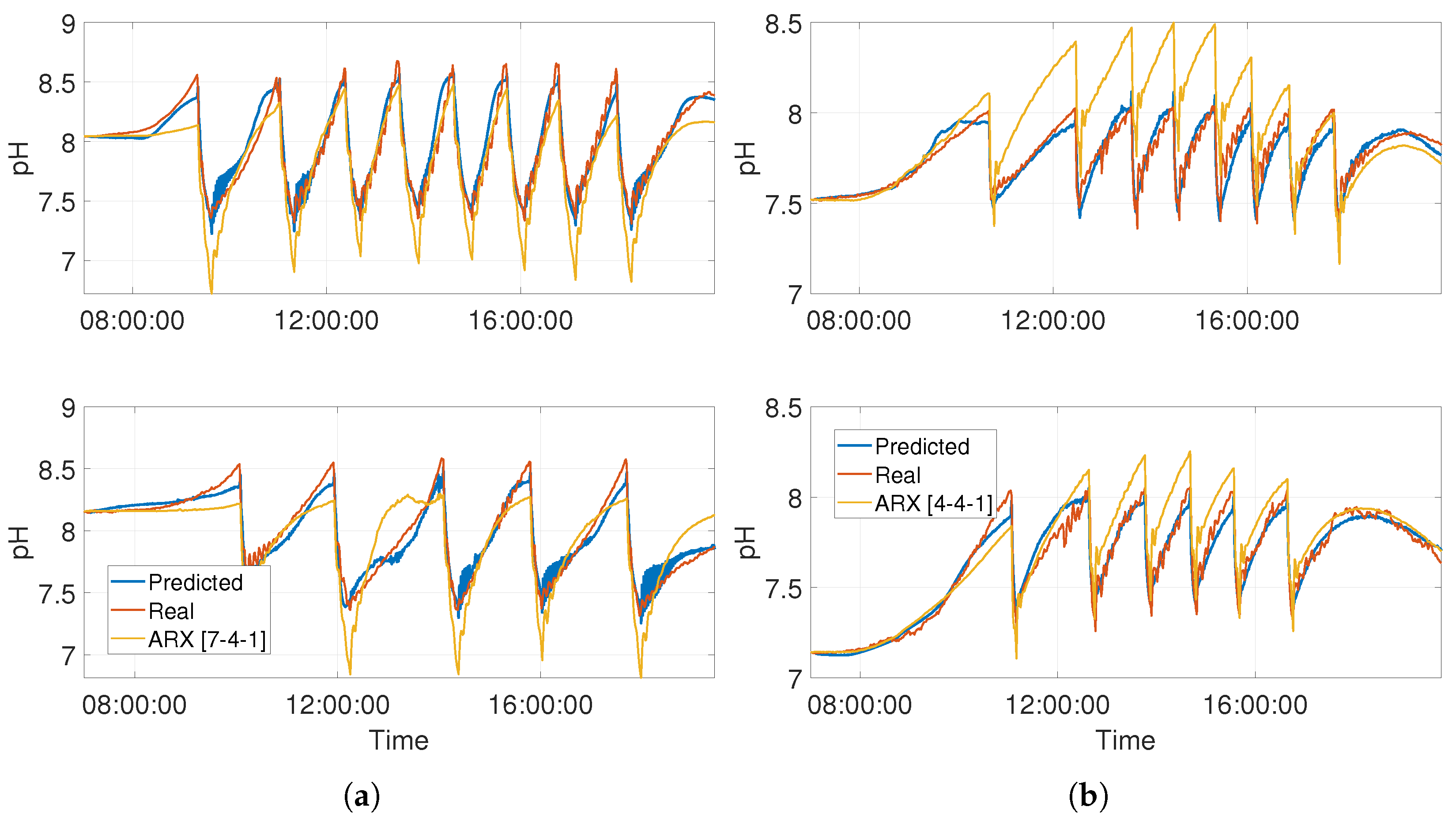
Compared to first-principles models, they are faster to run and simpler to re-calibrate on account of its smaller number of parameters and more straightforward formulation. For instance, compared to the previous reactor pH reference model developed in [24], the computation time for a full day’s simulation has been reduced from more than 4 min to approximately 0.4 s. On the other hand, they present a more general description of the system than any experimental linear model due to its nonlinear nature. The comparision with ARX models demonstrates the need for using nonlinear models to capture the dynamics of the system. Another interesting comparison may be in relation to LSTM networks. Such a simple model as the one presented is simpler algebraically and remarkably smaller in terms of the total number of parameters, being in any case able to fully capture the dynamics of the system.
The achieved results open many possibilities in the field of microalgae production. These models can be used as the basis of a nonlinear model-based predictive control algorithm to optimize the operating conditions. They can also be used for sensor fault detection, running concurrently with the plant. Regarding future works, it is interesting to extend the model to more production-influencing variables, such as DO, or to incorporate biomass concentration measurements that can make it more complete and adaptable. In a further perspective, the model could also be extended to predict the biomass concentration of the reactor itself in order to obtain a productivity model of the whole reactor. Moreover, the design of MPC algorithms based on the proposed models will be explored for the pH control in both types of reactors.

5. Conclusions

In this paper, two ANN models for pH prediction in microalgae photobioreactors have been developed. The results achieved demonstrate the potential of this type of model to characterize biological systems, showing high accuracy with relatively long prediction horizons. Specifically, the models obtained have been shown to provide accurate predictions over more than 12 h based solely on controllable or easily predictable variables as well as on their own predictions, which is more than enough not only for prediction purposes but also for simulation.
In addition, they adapt succesfully to freshwater and wastewater reactors, notwithstanding the differences on a dynamic level between them, which evidences its flexibility. With a similar methodology, the models can adapt to both type of reactors, which makes them easy to replicate in new facilities provided that a certain amount of historical data has been collected. The results are not only promising in the field of microalgae production but also in the field of biotechnology for modeling dynamic biological systems.

Author Contributions

Conceptualization, P.O.; methodology, P.O.; software, P.O.; validation, P.O.; formal analysis, P.O., M.B., J.L.G. and F.G.A.; writing—original draft preparation, P.O.; writing—review and editing, M.B., J.L.G. and F.G.A.; project administration, J.L.G. and F.G.A. All authors have read and agreed to the published version of the manuscript.

Funding

This work has been partially financed by the following projects: PID2020-112709RB-C21 project financed by the Spanish Ministry of Science and the Horizon Europe—the Framework Programme for Research and Innovation (2021–2027) under the agreement of grant no. 101060991 REALM. This research was supported by an FPU (Formación de Profesorado Universitario) scolarship from the Spanish Ministry of Science, Innovation and Universities to P.O.

Data Availability Statement

The data presented in this study are available on request from the corresponding author.

Acknowledgments

Thanks to M. Ruiz Arahal for his suggestions.

Conflicts of Interest

The authors declare no conflict of interest. The funders had no role in the design of the study; in the collection, analyses, or interpretation of data; in the writing of the manuscript; or in the decision to publish the results.

Abbreviations

The following abbreviations are used in this manuscript:
DODissolved Oxygen
ANNArtificial Neural Network
MPCModel Predictive Control
LSTMLong Short-Term Memory
NARXNonlinear AutoRegressive with eXogenous inputs
TDLTapped Delay Line
MSEMean Squared Error

References

  1. Guzmán, J.L.; Acién, F.G.; Berenguel, M. Modelling and control of microalgae production in industrial photobioreactors. Rev. Iberoam. Autom. Inform. Ind. 2020, 18, 1–18. [Google Scholar] [CrossRef]
  2. Acién Fernández, F.G.; Fernández Sevilla, J.M.; Molina Grima, E. Contribución de las microalgas al desarrollo de la bioeconomía. Mediterr. Econ. 2018, 31, 309–332. [Google Scholar]
  3. Hernández-Pérez, A.; Labbé, J.I. Microalgae, culture and benefits. Rev. Biol. Mar. Oceanogr. 2014, 49, 157–173. [Google Scholar] [CrossRef] [Green Version]
  4. Pittman, J.K.; Dean, A.P.; Osundeko, O. The potential of sustainable algal biofuel production using wastewater resources. Bioresour. Technol. 2011, 102, 17–25. [Google Scholar] [CrossRef] [PubMed]
  5. Abdel-Raouf, N.; Al-Homaidan, A.A.; Ibraheem, I.B. Microalgae and wastewater treatment. Saudi J. Biol. Sci. 2012, 19, 257–275. [Google Scholar] [CrossRef] [Green Version]
  6. De Andrade, G.A.; Berenguel, M.; Guzmán, J.L.; Pagano, D.J.; Acién, F.G. Optimization of biomass production in outdoor tubular photobioreactors. J. Process. Control. 2016, 37, 58–69. [Google Scholar] [CrossRef]
  7. Barceló-Villalobos, M.; Serrano, C.G.; Zurano, A.S.; García, L.A.; Maldonado, S.E.; Peña, J.; Fernández, F.G. Variations of culture parameters in a pilot-scale thin-layer reactor and their influence on the performance of Scenedesmus almeriensis culture. Bioresour. Technol. Rep. 2019, 6, 190–197. [Google Scholar] [CrossRef]
  8. Banerjee, S.; Ramaswamy, S. Dynamic process model and economic analysis of microalgae cultivation in open raceway ponds. Algal Res. 2017, 26, 330–340. [Google Scholar] [CrossRef]
  9. Sfez, S.; Van Den Hende, S.; Taelman, S.E.; De Meester, S.; Dewulf, J. Environmental sustainability assessment of a microalgae raceway pond treating aquaculture wastewater: From up-scaling to system integration. Bioresour. Technol. 2015, 190, 321–331. [Google Scholar] [CrossRef]
  10. Zhang, Q.; Li, X.; Guo, D.; Ye, T.; Xiong, M.; Zhu, L.; Liu, C.; Jin, S.; Hu, Z. Operation of a vertical algal biofilm enhanced raceway pond for nutrient removal and microalgae-based byproducts production under different wastewater loadings. Bioresour. Technol. 2018, 253, 323–332. [Google Scholar] [CrossRef]
  11. Sánchez-Zurano, A.; Rodríguez-Miranda, E.; Guzmán, J.L.; Acién-Fernández, F.G.; Fernández-Sevilla, J.M.; Molina Grima, E. Abaco: A new model of microalgae-bacteria consortia for biological treatment of wastewaters. Appl. Sci. 2021, 11, 998. [Google Scholar] [CrossRef]
  12. Mairet, F.; Muñoz-Tamayo, R.; Bernard, O. Adaptive control of light attenuation for optimizing microalgae production. J. Process. Control. 2015, 30, 117–124. [Google Scholar] [CrossRef]
  13. Sompech, K.; Chisti, Y.; Srinophakun, T. Design of raceway ponds for producing microalgae. Biofuels 2012, 3, 387–397. [Google Scholar] [CrossRef]
  14. Kazbar, A.; Cogne, G.; Urbain, B.; Marec, H.; Le-Gouic, B.; Tallec, J.; Takache, H.; Ismail, A.; Pruvost, J. Effect of dissolved oxygen concentration on microalgal culture in photobioreactors. Algal Res. 2019, 39, 101432. [Google Scholar] [CrossRef] [Green Version]
  15. De-Luca, R.; Bezzo, F.; Béchet, Q.; Bernard, O. Exploiting meteorological forecasts for the optimal operation of algal ponds. J. Process. Control. 2017, 55, 55–65. [Google Scholar] [CrossRef]
  16. González, J.; Rodríguez-Miranda, E.; Guzmán, J.L.; Acién, F.G.; Visioli, A. Temperature optimization in microalgae raceway reactors by depth regulation. Rev. Iberoam. Autom. Inform. Ind. 2022, 19, 164–173. [Google Scholar] [CrossRef]
  17. Posadas, E.; Morales, M.d.M.; Gomez, C.; Acién, F.G.; Muñoz, R. Influence of pH and CO2 source on the performance of microalgae-based secondary domestic wastewater treatment in outdoors pilot raceways. Chem. Eng. J. 2015, 265, 239–248. [Google Scholar] [CrossRef] [Green Version]
  18. Bernard, O.; Mairet, F.; Chachuat, B. Modelling of Microalgae Culture Systems with Applications to Control and Optimization. In Microalgae Biotechnology; Posten, C., Feng, C.S., Eds.; Springer International Publishing: Cham, Switzerland, 2016; pp. 59–87. [Google Scholar] [CrossRef]
  19. García-Mañas, F.; Guzmán, J.L.; Berenguel, M.; Acién, F.G. Biomass estimation of an industrial raceway photobioreactor using an extended Kalman filter and a dynamic model for microalgae production. Algal Res. 2019, 37, 103–114. [Google Scholar] [CrossRef]
  20. Fernández, I.; Acién, F.G.; Berenguel, M.; Guzmán, J.L. First principles model of a tubular photobioreactor for microalgal production. Ind. Eng. Chem. Res. 2014, 53, 11121–11136. [Google Scholar] [CrossRef]
  21. Pawlowski, A.; Guzmán, J.L.; Berenguel, M.; Acién, F.G. Control system for pH in raceway photobioreactors based on Wiener models. IFAC-PapersOnLine 2019, 52, 928–933. [Google Scholar] [CrossRef]
  22. Pawlowski, A.; Fernández, I.; Guzmán, J.L.; Berenguel, M.; Acién, F.G.; Dormido, S. Event-based selective control strategy for raceway reactor: A simulation study. IFAC-PapersOnLine 2016, 49, 478–483. [Google Scholar] [CrossRef]
  23. Fernández, I.; Acién, F.G.; Fernández, J.M.; Guzmán, J.L.; Magán, J.J.; Berenguel, M. Dynamic model of microalgal production in tubular photobioreactors. Bioresour. Technol. 2012, 126, 172–181. [Google Scholar] [CrossRef] [PubMed]
  24. Fernández, I.; Acién, F.G.; Guzmán, J.L.; Berenguel, M.; Mendoza, J.L. Dynamic model of an industrial raceway reactor for microalgae production. Algal Res. 2016, 17, 67–78. [Google Scholar] [CrossRef]
  25. Rodríguez-Miranda, E.; Acién, F.G.; Guzmán, J.L.; Berenguel, M.; Visioli, A. A new model to analyze the temperature effect on the microalgae performance at large scale raceway reactors. Biotechnol. Bioeng. 2021, 118, 877–889. [Google Scholar] [CrossRef]
  26. Ifrim, G.A.; Titica, M.; Cogne, G.; Boillereaux, L.; Legrand, J.; Caraman, S. Dynamic pH model for autotrophic growth of microalgae in photobioreactor: A tool for monitoring and control purposes. AIChE J. 2014, 60, 585–599. [Google Scholar] [CrossRef]
  27. Pawlowski, A.; Mendoza, J.L.; Guzman, J.L.; Berenguel, M.; Acien, F.G.; Dormido, S. Effective utilization of flue gases in raceway reactor with event-based pH control for microalgae culture. Bioresour. Technol. 2014, 170, 1–9. [Google Scholar] [CrossRef]
  28. Rodríguez-Miranda, E.; Guzmán, J.; Berenguel, M.; Acién, F.; Visioli, A. Diurnal and nocturnal pH control in microalgae raceway reactors by combining classical and event-based control approaches. Water Sci. Technol. 2020, 82, 1155–1165. [Google Scholar] [CrossRef]
  29. Jordan, M.I.; Mitchell, T.M. Machine learning: Trends, perspectives, and prospects. Sci. 2015, 349, 255–260. [Google Scholar] [CrossRef]
  30. Rajendra, P.; Brahmajirao, V. Modeling of dynamical systems through deep learning. Biophys. Rev. 2020, 12, 1311–1320. [Google Scholar] [CrossRef]
  31. Kiš, K.; Klaučo, M. Neural network based explicit MPC for chemical reactor control. Acta Chim. Slovaca 2020, 12, 218–223. [Google Scholar] [CrossRef] [Green Version]
  32. Pon Kumar, S.S.; Tulsyan, A.; Gopaluni, B.; Loewen, P. A deep learning architecture for predictive control. IFAC-PapersOnLine 2018, 51, 512–517. [Google Scholar] [CrossRef]
  33. Correa, I.; Drews, P.; Botelho, S.; De Souza, M.S.; Tavano, V.M. Deep learning for microalgae classification. In Proceedings of the 16th IEEE International Conference on Machine Learning and Applications, ICMLA 2017, Cancun, Mexico, 18–21 December 2017; Volume 2017, pp. 20–25. [Google Scholar] [CrossRef]
  34. Otálora, P.; Guzmán, J.L.; Acién, F.G.; Berenguel, M.; Reul, A. Microalgae classification based on machine learning techniques. Algal Res. 2021, 55, 102256. [Google Scholar] [CrossRef]
  35. Otálora, P.; Guzmán, J.L.; Berenguel, M.; Acién, F.G. Dynamic Model for the pH in a Raceway Reactor using Deep Learning techniques. In Proceedings of the CONTROLO 2020. Lecture Notes in Electrical Engineering; Gonçalves, J.A., Braz-César, M., Coelho, J.P., Eds.; Springer: Berlin/Heidelberg, Germany, 2020; Volume 695, pp. 190–199. [Google Scholar]
  36. Caparroz, M.; Otálora, P.; Guzmán, J.L.; Berenguel, M. Modelado y control adaptativo del pH en reactores raceway para la producción de microalgas. In Proceedings of the XLIII Jornadas de Automática, Logroño, Spain, 7–9 September 2022; pp. 333–340. [Google Scholar]
  37. Kay, R.A.; Barton, L.L. Microalgae as Food and Supplement. Crit. Rev. Food Sci. Nutr. 1991, 30, 555–573. [Google Scholar] [CrossRef]
  38. Xie, H.; Tang, H.; Liao, Y.H. Time series prediction based on NARX neural networks: An advanced approach. In Proceedings of the 2009 International Conference on Machine Learning and Cybernetics, Baoding, China, 12–15 July 2009; Volume 3, pp. 1275–1279. [Google Scholar] [CrossRef]
  39. Boussaada, Z.; Curea, O.; Remaci, A.; Camblong, H.; Mrabet Bellaaj, N. A Nonlinear Autoregressive Exogenous (NARX) Neural Network Model for the Prediction of the Daily Direct Solar Radiation. Energies 2018, 11, 620. [Google Scholar] [CrossRef] [Green Version]
  40. Cerinski, D.; Baleta, J.; Mikulčić, H.; Mikulandrić, R.; Wang, J. Dynamic modelling of the biomass gasification process in a fixed bed reactor by using the artificial neural network. Clean. Eng. Technol. 2020, 1, 100029. [Google Scholar] [CrossRef]
  41. Song, H.; Shan, X.; Zhang, L.; Wang, G.; Fan, J. Research on identification and active vibration control of cantilever structure based on NARX neural network. Mech. Syst. Signal Process. 2022, 171, 108872. [Google Scholar] [CrossRef]
  42. Kim, P. MATLAB Deep Learning; Apress: Berkeley, CA, USA, 2017. [Google Scholar] [CrossRef]
  43. Ljung, L. System Identification Toolbox; Math Works: Natick, MA, USA, 1995. [Google Scholar]
Figure 1. Raceway photobiorreactors modeled in this work.
Mathematics 11 01614 g001
Figure 2. NARX ANN sample diagram with k predictor TDLs and j output TDLs.
Mathematics 11 01614 g002
Figure 3. Sample data from four consecutive days from the freshwater reactor.
Mathematics 11 01614 g003
Figure 4. Validation results for each of the models using two days of the test set. (a) Freshwater model validation results, (b) Wastewater model validation results.
Mathematics 11 01614 g004
Table 1. Sensors integrated in the reactors.
MeasurementModelRangePrecision
pHCrison 5342T[0–14]0.01
Medium temperatureCrison 5342T[0–80] °C0.1 °C
Dissolved oxygenMettler Toledo InPro 6050[30–Sat.] ppb30 ppb
Medium levelWenglor UMD402U035[0–30] cm0.1 mm
CO 2 injectionSMC PFM725S-C8-F[0.5–25] L/min0.1 L/min
Air injectionSMC PFMB7501-F04-F[5–500] L/min1 L/min
Ambient temperatureONSET S-THB-M008[−40–75] o C 0.21 °C
HumidityONSET S-THB-M008[10–90] %0.1%
Solar radiationONSET S-LIB-M003[0–1280] W / m 2 10 W / m 2
Table 2. Maximum and minimum values from each variable used to normalize the data.
VariableMaximum (Freshwater)Minimum (Freshwater)Maximum (Wastewater)Minimum (Wastewater)
pH11.337.138.077.11
Medium level19.20 cm13.16 cm15.23 cm13.29 cm
CO 2 injection13.49 L/min0 L/min12.00 L/min0 L/min
Solar radiation1080.94 W/ m 2 0 W/ m 2 1060.39 W/ m 2 0 W/ m 2
Table 3. TDLs applied to each model input.
VariableTDL
pH(k−1):(k−2)
Medium level(k−1):(k−2)
CO 2 injection(k−5):(k−6)
Solar radiation(k−1):(k−2)
Table 4. Model test performance (MSE) for each hidden layer size.
Hidden Layer SizeFreshwater ModelWastewater ModelNumber of Parameters
50.02080.013051
60.03410.040961
70.01950.050071
80.04290.010681
90.03670.083691
100.02910.0449101
110.04040.0532111
120.04170.0325121
130.03840.0225131
140.03830.0517141
150.01920.0601151
Table 5. Performance metrics for each model.
Freshwater ModelWastewater Model
Test Model Fit (%)71.3473.75
General Model Fit (%)63.9162.76
Test MSE0.01920.0106
[4-4-1] ARX Model Fit (%)−19.4310.64
[4-4-1] ARX MSE0.15310.0301
[8-8-1] ARX Model Fit (%)−2.32−198.00
[8-8-1] ARX MSE0.11020.3406
Best-fit ARX Model Fit (%)41.76−60.26
Best-fit ARX MSE0.03570.0971
Disclaimer/Publisher’s Note: The statements, opinions and data contained in all publications are solely those of the individual author(s) and contributor(s) and not of MDPI and/or the editor(s). MDPI and/or the editor(s) disclaim responsibility for any injury to people or property resulting from any ideas, methods, instructions or products referred to in the content.

