Intelligent Analysis of Construction Costs of Shield Tunneling in Complex Geological Conditions by Machine Learning Method

Abstract

The estimation of construction costs for shield tunneling projects is typically based on a standard quota, which fails to consider the variation of geological parameters and often results in significant differences in unit cost. To address this issue, we propose a novel model based on a random forest machine learning procedure for analyzing the construction cost of shield tunnelling in complex geological conditions. We focus specifically on the unit consumption of grease, grouting, labor, water, and electricity. Using a dataset of geotechnical parameters and consumption quantities from a shield tunneling project, we employ KNN and correlation analysis to reduce the input dataset dimension from 17 to 6 for improved model accuracy and efficiency. Our proposed approach is applied to a shield tunneling project, with results showing that the compressive strength of geomaterial is the most influential parameter for grease, labor, water, and electricity, while it is the second most influential for grouting quantity. Based on these findings, we calculate the unit consumption and cost of the tunnelling project, which we classify into three geological categories: soil, soft rock, and hard rock. Comparing our results to the standard quota value, it is found that the unit cost of shield tunneling in soil is slightly lower (6%), while that in soft rock is very close to the standard value. However, the cost in the hard rock region is significantly greater (38%), which cannot be ignored in project budgeting. Ultimately, our results support the use of compressive strength as a classification index for shield tunneling in complex geological conditions, representing a valuable contribution to the field of tunneling cost prediction.

1. Introduction

Project budgets during the bidding stage and project final accounts after completion are the two important steps of construction project management [1,2] of shield tunneling projects. The core of construction project management is the investment estimation of the construction cost for shield tunneling engineering [3,4]. The investment estimation of the construction cost governs project profitability. Since it is a crucial component of the economic analysis of a subway line or underground tunnel, the cost of a shield tunneling project has a substantial impact on the overall economic benefit. The accurate cost prediction of tunneling projects is critical, as it can provide a powerful source of help for reducing the project costs and optimizing construction management. Therefore, it is essential to thoroughly examine the cost prediction in order to increase its speed and accuracy and make correct investment decisions [5].

In practice, the shield tunneling project cost is normally estimated by the use of an official budget standard, which defines the quota of main construction consumption containing the unit quantities of grease, grouting, labor, and so forth. Theoretically, the total construction cost can be calculated as the standard consumption multiplied by the unit price. However, concerning the tunneling, quantities of consumption exhibit an obvious relationship with the geological condition of the construction site [6,7]. Consequently, the usual computation procedure of shield tunneling without considering different geological conditions will lead to great errors in the construction cost. Especially in underground tunneling projects, the excavation site usually has composite geological layers. This implies proposing a new computation method with the consideration of influences of geotechnical parameters on the total cost [8,9,10].

Numerous studies have been devoted to the factors that affect tunneling costs by researchers in recent years. Aiming at avoiding unexpected variations of time and cost during the construction process, different studies have been published concerning the influences of composite geological conditions [11,12,13]. By the use of mathematical models [14,15], the random process and time it takes for the excavation process have been fully discussed by considering the geological conditions around the tunnel route. Besides, in order to gather information on the geological conditions in the complex tunneling region, in situ equipment was applied by Carrière et al. [16] for pilot-drilling, subsurface-boring, and advanced geophysical prospecting. Daraei et al. [17] proposed the application of value engineering principles to decrease construction costs and increase safety in tunnel construction projects in Iraqi Kurdistan, demonstrated through the optimization of the Heybat Sultan twin tunnels project. Particularly, Mahmoodzadeh et al. [18] has proposed a novel model to estimate the construction time and cost in tunneling projects. The influences of uncertain geological conditions in tunneling construction on the time and cost were analyzed by applying the Markov chain and considering opinions of experts.

In addition, with the development of artificial intelligence [19,20], various machine learning algorithms have been successfully applied to the prediction of construction cost. Ye [21] established an intelligent algorithm for the construction cost estimation, which was developed from the Particle Swarm Optimization (PSO) Guided BP Neural Network. Combined with the Support Vector Machine (SVM) method, the construction cost of substations has been successfully predicted by a PSO-based procedure in the Ref. [22]. Considering the gray fuzzy theory, a gray fuzzy predictive model was proposed by Liu et al. [23] to calculate the cost of an unfinished construction. The Decision Aids for Tunneling (DAT) [24] is a computer-based tool which has also been widely used for computing the distributions of tunnelling cost and time, considering uncertainties of the geological conditions. On the other hand, aiming at using the official quota for the consumption quantities in complex geological conditions, the degrees of impact of the geotechnical parameters [25,26] are essential for the classification, indicating the application of the random forest method [27]. Concerning the application of machine learning algorithms for engineering practice, development of a user-friendly software tool has been considered by researchers [28,29,30]. The software is easily used by engineers and practitioners without the need for extensive knowledge of the underlying machine learning algorithms.

As an ensemble learning technique for classification, regression, and other problems, random forests build a large number of decision trees during the training process [31,32,33]. The result of the random forest for classification (RFC) tasks is the class that the majority of the trees choose [34,35]. For regression tasks (RFR), the mean or average forecast of each individual tree is returned [36,37]. Random choice forests correct the tendency of decision trees to overfit their training set. The potential of forecasting the fatty acids and tocopherols content has been explored by Rajković et al. [38], by combining two machine learning methods, namely the artificial neural network (ANN) and random forest regression (RFR) algorithms. In particular, the random forest method can be used to compute the feature importance score of input datasets due to the bootstrap structure [39,40,41]. Gu et al. [42] carried out a random forest-based computation and found that the annual average daily traffic on a minor road from the roadway traffic characteristics group makes the highest contribution to rear-end crashes. Similarly, the feature importance of different variables has also been evaluated by the random forest procedure for fatal fall-from-heights accidents [43], vegetation mapping in savannah regions [44] and contributions from LiDAR and orthoimagery data to map urban objects [45].

Considering the difficulty of the classification of budget quotas in complex geological conditions, the present study is devoted to analyzing the influences of geotechnical parameters on the main unit consumption in shield tunneling. The excavation consumption and geotechnical data were collected from a shield tunneling project in China, in which different soil and rock geological layers are involved. In order to obtain the most impactful geotechnical parameter in complex conditions, the random forest machine learning technique is employed with the consumption factor as the target in this study. Referring to the opinions of experts, four consumption factors for shield tunneling, quantity of grease, grouting, labor and water and electricity are studied for different geological conditions. The main purpose of our study was to find out the most impactful geological parameter and propose a new budget quota for classification. Thus, the random forest classification algorithm is applied and the collected data will be classified in different categories. In comparison with the DAT method, the proposed random forest-based model is data-driven, which allows us to take into account the full range of geotechnical parameters and their interactions in a more comprehensive manner. It does not require specific knowledge and can be easily implemented in engineering practice. The most influential geotechnical parameter on the consumption of shield tunneling is obtained from the comprehensive result of four factors by the random forest procedure. Consequently, the shield tunneling consumption in different geological conditions is computed with the classification of the parameter, which will provide the basis for novel quotas in this situation.

The present paper is organized in the following way. In Section 2, the background of the shield tunneling project is briefly introduced, and the collection and ordering of geotechnical and consumption data are also described. In order to improve the computation accuracy and efficiency, the dimension of the datasets is reduced before model training. Section 3 is devoted to recalling the principle formulation of the random forest algorithm, as well as the general flowchart of this machine learning method in analysis of the construction cost of shield tunneling in complex geological conditions. In Section 4, the constructed random forest model is applied to calculate the importance score of considered geotechnical parameters for four consumption factors. The accuracy of the proposed method is accessed by comparison with the unit consumption and cost in the soil, soft rock and hard rock conditions with those of the standard one. In the last section, some concluding points are provided.

2. Problem Description and Data Pre-Processing

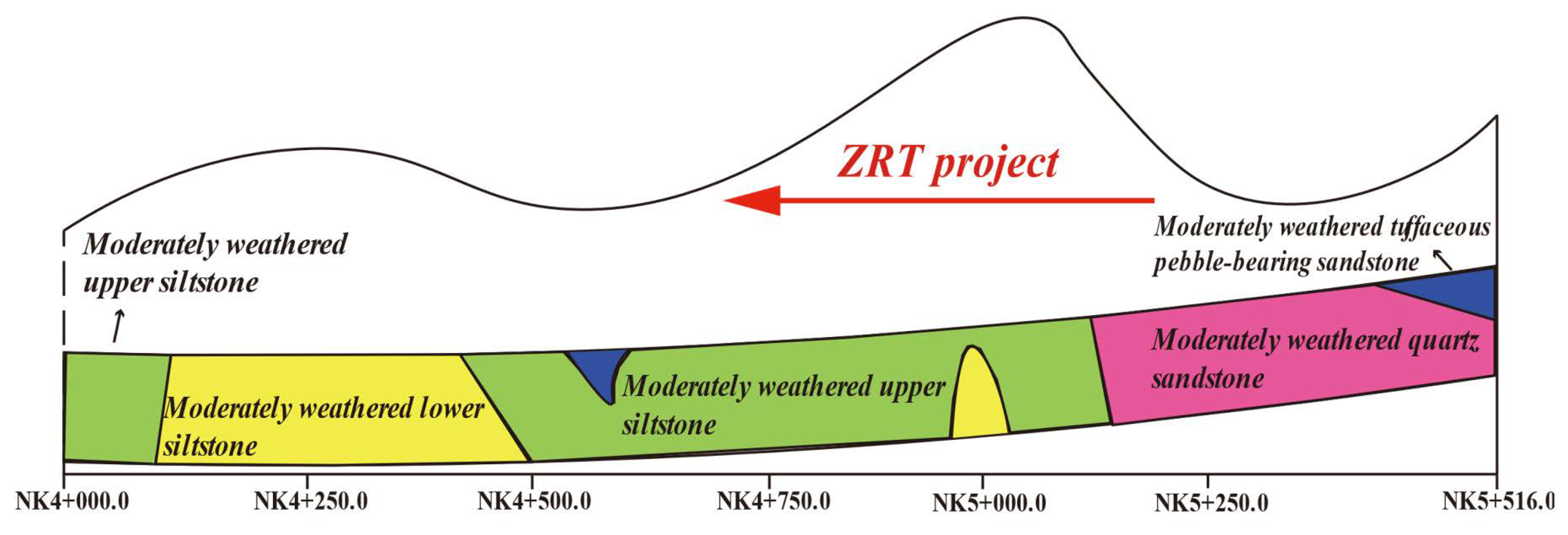
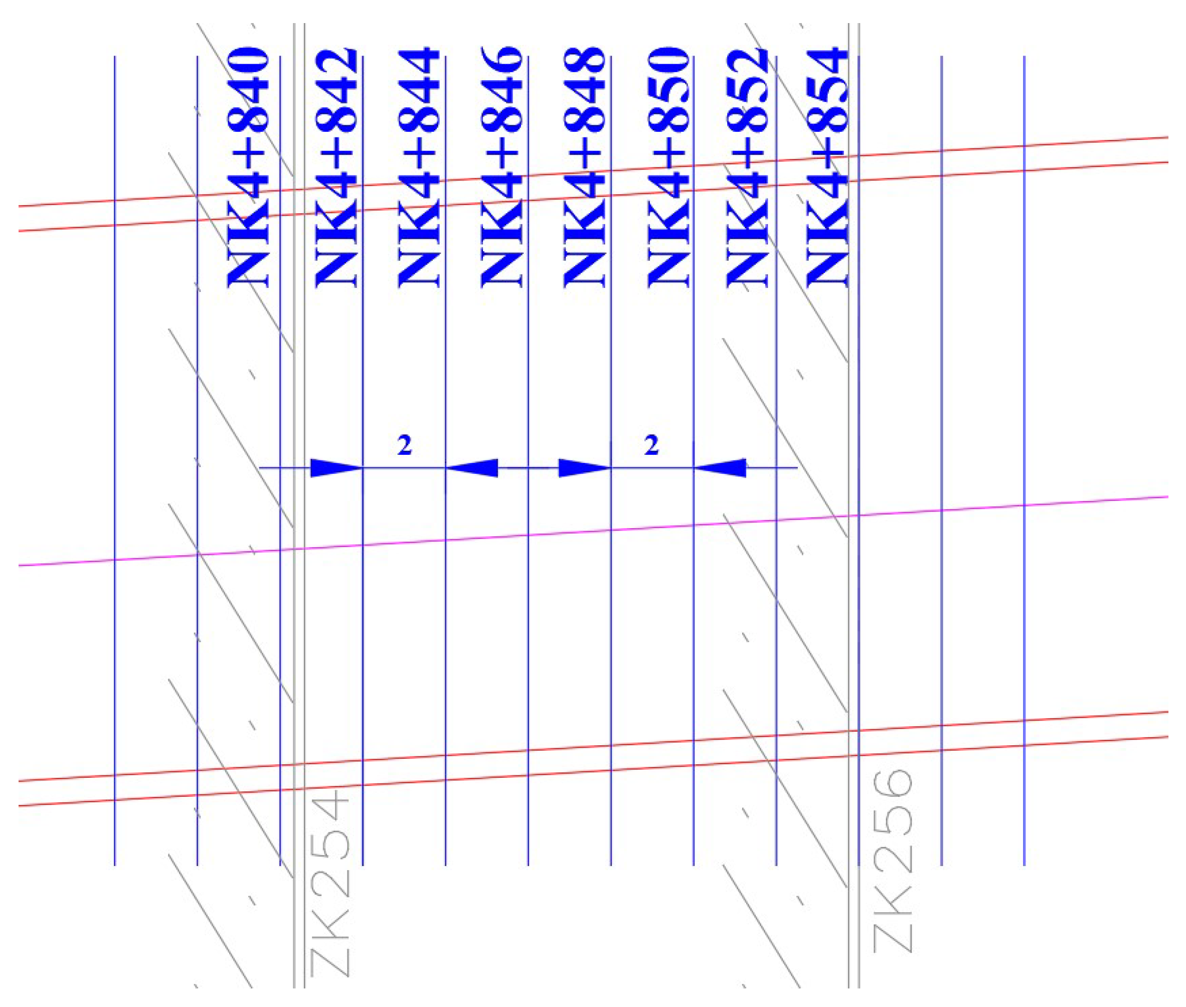
2.1. Background of the Project

The present study is based on data and reports from the Zhijiang Road Tunneling (ZRT) project in Hangzhou, China, as shown in Figure 1. The tunnel was excavated using a combination of shield tunneling (mud–water balancing shield machine with inner diameter 14.5 m and outer diameter 15.03 m) and open-cut methods. The shield tunneling portion, marked by the red point in Figure 1, spans a distance of 3.6 km and is divided into east and west sections.

Based on the geological engineering investigation report, the tunnel geology of the entire west section is primarily composed of extremely soft and soft rock, where moderately weathered argillaceous siltstone accounts for approximately 53% and moderately weathered tuffaceous sandstone accounts for about 19%. In the east tunneling excavation section, hard rock predominates, including moderately weathered siltstone accounting for 60% and moderately weathered quartz sandstone accounting for 10% (Figure 2).

2.2. Collection of Geological Data and Tunneling Consumption

The distribution of main geological conditions along the east tunneling part of ZRT project is displayed in Figure 3. We take it as an example to explain the collection and preparation of geological data on site of the project and of the shield operational consumption. Noticing that the width of standard shield segments is 2 m, the datasets of tunneling consumption are consequently collected per 2 m. As shown in Figure 4, the arrangement of geological data and material consumption are in the same order of shield segments, which is crucial for training the random forest model developed in our study.

In order to improve the the generalization ability of the constructed model in the present study, 17 geological parameters in the geological report are all taken into account. The statistical information of geological parameters which will be analyzed in the following machine learning model is provided in

Table 1. Statistical information of 17 geological parameters of different layers.

Geotechnical Parameters and Abbreviations	Soil 1	Soil 2	Soil 3	Soil 4	…	Rock 9
Moisture content ($W_0$ %)	28.98	45.24	41.87	41.59	…	-
Natural density ($\gamma$ kN/m${}^3$)	19.10	17.40	17.40	17.80	…	26.00
Specific gravity ($G_s$)	2.70	2.73	2.73	2.73	…	-
Void ratio ($\mathrm{e}$)	0.80	1.30	1.15	1.23	…	0.032
Saturability ($S_r$)	95.66	95.25	96.12	92.47	…	-
Liquid limit (WL)	-	40.51	38.64	39.75	…	-
Plastic limit (WP)	-	24.34	23.94	23.97	…	-
liquidity index (IL)	-	16.17	14.70	15.77	…	-
plasticity index (IP)	-	1.32	1.20	0.97	…	-
Bearing capacity (fak kPa)	130	65	65	100	…	3500
Modulus of compressibility ($E_s$ MPa)	7.0	2.3	2.4	4.0	…	-
Lateral pressure coefficient ($k_0$ MPa${}^{-1}$)	0.40	0.58	0.58	0.54	…	0.25
Horizontal permeability coefficient (KH cm/s)	$1.0\times {10}^3$	$4.0\times {10}^6$	$2.0\times {10}^6$	$2.0\times {10}^6$	…	$3.0\times {10}^6$
Vertical permeability coefficient (KV cm/s)	$9.0\times {10}^4$	$3.0\times {10}^6$	$1.5\times {10}^6$	$1.5\times {10}^6$	…	$2.5\times {10}^6$
Cohesion (c kPa)	3.0	13.0	13.0	24.0	…	450
Friction angle ($\mathsf{\varphi }$ ${}^{\circ }$)	25	9.5	10	12	…	43
Compressive strength ($\mathsf{\sigma }$ MPa)	5000	$4\times 10$	9.4021	0.9954	…	60.40

for different geological layers. For the sake of simplicity, the abbreviations of each geotechnical parameter are also provided in this table, and will be used in the following part of this study. Besides, it can be found that some specific values of the geotechnical parameters are missing, so additional pre-processing for the missing values is needed. The objective of this paper concerns the influence of complex geological conditions on economic factors in shield tunneling, so the feature importance of different geological parameters should be considered. Thus, it would be better to find out the main influence geological factors, providing a basis for the cost classification of budgets.

Similarly, the main consumption factors in the tunneling process are also recorded per segment (2 m). In the present paper, four main consumption indicators, the amount of grease, grouting, labor and water and electricity, are studied for the purpose of economic classification in complex geological conditions. From this perspective, the main components of each indicator are given in

Table 2. Statistical information of 4 concerned consumption indicators.

Consumption Indicator	Components	Unit Price 1	Index
Grease	Tail grease	17.5	$Y_1$
	EP2 grease	25.0	$Y_2$
	Seal grease	55.0	$Y_3$
Grouting	Grouting	1.3–1.8	$Y_4$
Labor	Labor	135.0	$Y_5$
Water & electricity	Water	4.27	$Y_6$
	Electricity	0.78	$Y_7$

¹ The currency for the unit price is CNY.

based on the official Quota Booklet of shield tunneling (Version 2018). The unit prices of each consumption component are also provided for the computation of construction cost in the following part. The key influencing economic consumptions are arranged in the order of shield segment, as those of geological data. Moreover, the objective consumption indicators are ordered by the $Y_i$ index in order to be implemented in the random forest program.

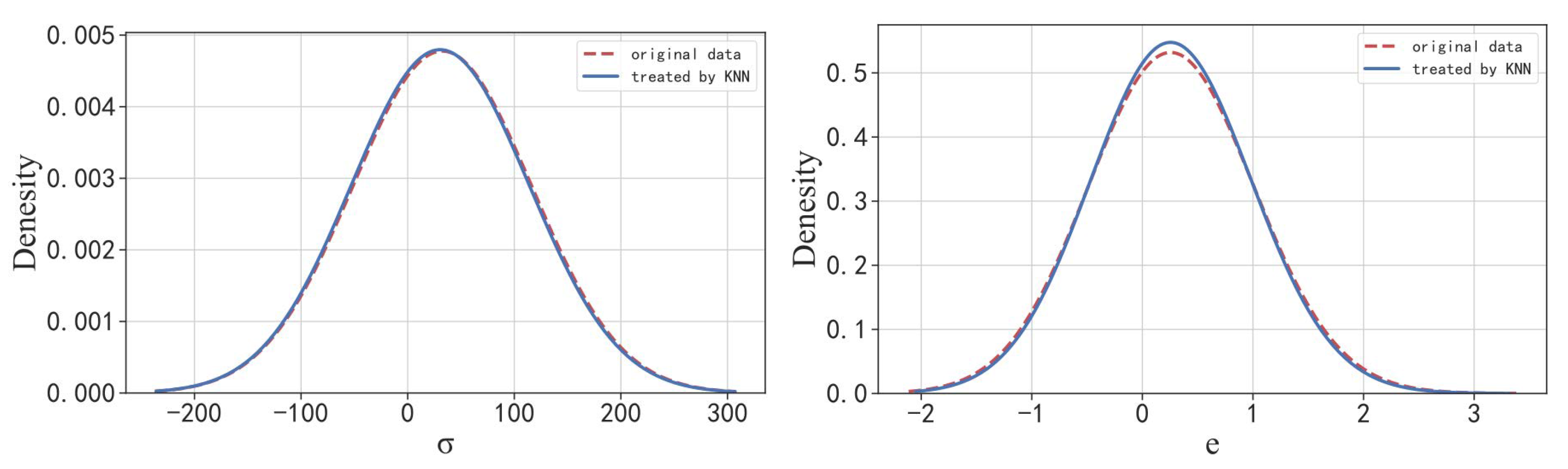
2.3. Pre-Processing of the Datasets

For the purpose of determination of shield tunneling consumption in complex geological conditions, especially for the four indicators in Table 2, the collected data will be used in a random forest-based procedure to train the model. The accuracy of the prediction model is significantly influenced by the quality of the input data. Before the implementation, data pre-processing is needed for the missing and abnormal values.

As shown in Figure 5, the values of geotechnical parameters are displayed in the arranged order of shield segment. The abbreviations for the concerned geotechnical parameters are given in Table 1. It can be seen that there are too much missing data for 8 parameters (W${}_0$, G${}_s$, S${}_r$, WL, WP, IP, IL and E${}_s$), which will be neglected for the following analysis. Besides, some recorded values for tunneling consumption data could be abnormal due to incorrect recording or other reasons. Those abnormal values (too large or too small) will be removed, and the missing data of $\mathsf{\sigma }$ and $\mathrm{e}$ will be replaced by that calculated by the KNN algorithm (k-Nearest Neighbor) [46]. The distribution of original data (red dash line) and that treated by the KNN algorithm (blue solid line) are plotted in Figure 6, respectively. It is obviously seen that the distribution of compressive strength ($\mathsf{\sigma }$) and void ratio ($\mathrm{e}$) are not changed, and they can be accepted for the following analysis by the random forest procedure.

Moreover, in the random forest program, the performance of the random forest model will get worse if the degree of correlation between involved geotechnical parameters is greater. In order to improve the accuracy of the random forest procedure, the collected geological data also need to be analyzed for the correlation coefficient. Consequently, the correlation matrix is used to display the correlation coefficients among all the geological parameters, before being implemented in the program. The heat map (Figure 7), also known as the correlation coefficient map, can visually judge the magnitude of the correlation between variables based on the color of different squares on the heat map. The correlation coefficient can be calculated directly by the following formulation:

$$\rho =\frac{Cov\left(X_1,X_2\right)}{\sqrt{D{X}_1,D{X}_2}}=\frac{E\left(X_1{X}_2\right)-E\left(X_1\right)·E\left(X_2\right)}{\sqrt{D{X}_1,D{X}_2}}$$

(1)

where $Cov$ denotes the covariance and E is the mathematical expectation. By the use of the heat map, the involved geotechnical features with high correlation can be screened out to prevent overfitting in the random forest model. As shown in Figure 7, the correlation coefficients of nine different geotechnical variables (after the remove of missing data) are displayed in the form of a heat map by different colors. Notice that the abbreviations for the parameters have already been provided in Table 1.

It is clear from Figure 7 that any of the nine features recovered exhibit a high degree of association. The nine datasets will again be shrunk in dimension to avoid features with strong correlations that would have a significant impact on the obtained prediction. It is demonstrated that there is a strong correlation between the cohesion and bearing capacity (0.86), natural density and friction angle (0.95), and horizontal and vertical permeability coefficients (1.00). Consequently, we only need to reserve one of the mentioned pair of geotechnical parameters. In practice, the natural density and bearing capacity are important geological parameters according to experts and need to be reserved. By reserving the vertical permeability coefficient, nine parameters are reduced to six for the variable importance analysis by random forest. Figure 8 displays the final data preparation after reductions from 17 to 6 geotechnical input parameters for the model training. Each of the input data contains 1979 sets.

3. Methodology

Random forests is an ensemble learning method for classification, regression and other tasks that operates by constructing a multitude of decision trees at the training time. The class that the majority of the trees chose is the output of the random forest for classification tasks. The mean or average prediction of each individual tree is returned for regression tasks. The tendency of decision trees to overfit their training set is corrected by random decision forests. By randomly sampling the sample data, multiple different decision trees are formed, and then the results are combined to obtain the prediction results of the random forest. The variable importance in the objective tunneling consumption indicators will be calculated by the constructed model in this paper. Thus, this section is devoted to the basic principle of the random forest model and the algorithm applied to this study.

3.1. Principle Technique of Random Forest

Decision Trees is a non-parametric supervised learning method. The goal is to create a model that predicts the value of a target variable by learning simple decision rules inferred from the data features. A tree can be seen as a piecewise constant approximation. Given a training set $\mathit{X}=\{X_1,X_2,\dots ,X_n\}$ with responses $\mathit{Y}=\{Y_1,Y_2,\dots ,Y_n\}$, a decision tree recursively partitions the feature space such that the samples with the same labels or similar target values are grouped together.

Let the data at node m be represented by $Q_m$ with $n_m$ samples. For each candidate split $\theta =(j,t_m)$ consisting of a feature j and threshold $t_m$, partition the data into $Q_m^l\left(\theta \right)$ and $Q_m^r\left(\theta \right)$ subsets:

$$\begin{array}{cc}\hfill Q_m^l\left(\theta \right)& =\{(x,y)\mid x_j\le t_m\}\hfill \\ \hfill Q_m^r\left(\theta \right)& =Q_m\setminus Q_m^l\left(\theta \right)\hfill \end{array}$$

(2)

The quality of a candidate split of node m is then computed using an impurity function or loss function H, the choice of which depends on the task being solved

$$G(Q_m,\theta )=\frac{n_m^l}{n_m}H\left(Q_m^l\left(\theta \right)\right)+\frac{n_m^r}{n_m}H\left(Q_m^r\left(\theta \right)\right)$$

(3)

Select the parameters that minimises the impurity

$${\theta }^{*}={\mathrm{argmin}}_{\theta }G(Q_m,\theta )$$

(4)

Recurse for subsets $Q_m^l\left({\theta }^{*}\right)$ and $Q_m^r\left({\theta }^{*}\right)$ until the maximum allowable depth is reached $n_m<{\min }_{samples}$ or $n_m=1$.

If a target is a classification outcome taking on values 0, 1, …, K − 1, for node m, let

$$p_{mk}=\frac{1}{n_m}\sum _{y\in Q_m}I(y=k)$$

(5)

be the proportion of class k observations in node m. Two common measures of impurity are the Gini index:

$$H\left(Q_m\right)=\sum _k{p}_{mk}(1-p_{mk})$$

(6)

and log loss or Entropy:

$$H\left(Q_m\right)=-\sum _k{p}_{mk}log\left(p_{mk}\right)$$

(7)

The Random Forest algorithm [33] is a classification algorithm composed of multiple decision trees, with each tree producing a category that contributes to the final output category. It is built using the bagging method and categorical regression trees and has been successfully used in various disciplines (see Figure 9). Random forests consist of different decision trees that are independent of each other. When a sample is inputted, each tree in the forest will make a decision and vote to determine the best category. Typically, $\sqrt{p}$ features are used in each split for classification problems with p features. However, each problem requires tuning to identify the best values for these parameters.

Each dataset is used to construct the largest decision tree possible without any additional processing. Then, the information gain is determined using the entropy or Gini index in the randomly selected feature factors. After computing each accuracy information, the candidate feature factor with the highest information gain (entropy or Gini) among them is divided. These stages are iteratively repeated until the entropy or Gini becomes smaller than the predetermined value, resulting in the development of a random forest algorithm with n decision trees. The training data for feature identification is then classified using the established random forest model, and the decision trees in the forest vote to determine the best classification prediction.

The random forest approach can be utilized to order the relevance of variables in a classification or regression task in a natural way. During training, the error is tracked and averaged over the forest. The contribution (Gini) can be computed using the Gini index. After training, the jth feature values are permuted among the training data, and the error is computed once again on this perturbed dataset to determine the jth feature’s relevance. By averaging the difference between before and after the permutation over all trees, the importance score for the jth feature is calculated. The score is standardized using the standard deviation of these differences.

We take the Gini index as a measure to show the calculation of variable importance. Considering n categories, the weight of the k-th category can be computed from Equation (6). For feature j, the change value of feature j at node m (${\mathrm{VI}}_{jm}$) is obtained as:

$${\mathrm{VI}}_{jm}={\mathrm{GI}}_m-{\mathrm{GI}}_l-{\mathrm{GI}}_r$$

(8)

where ${\mathrm{GI}}_m$ is the Gini index before branch; ${\mathrm{GI}}_l$ and ${\mathrm{GI}}_r$ is the new Gini index after the node m. The normalized value of the contribution of feature j is the importance score of feature j, which is calculated as follows:

$${\mathrm{VI}}_j^{\prime }=\frac{{\mathrm{VIM}}_j}{{\sum }_{i=1}^c{\mathrm{VIM}}_i}$$

(9)

The detailed derivation of variable importance can be found in the Ref. [42].

Actually, the random forest model is used to rank the importance of variables (geotechnical parameters) (Equation (9)) by a classification problem in the present paper meaning, that the most impactful geotechnical parameter can be selected for the quota of budget of shield tunneling in complex geological conditions.

3.2. Application of the Random Forest-Based Method in Analysis of Tunneling Consumption in Complex Geological Conditions

The considered economic factors (consumption of grease, grouting, labor and water and electricity) in shield tunneling project will be analyzed by the random forest-based model. The contributions of geological parameters (feature importance) are expected to be calculated, so that the proof for classification in complex geological conditions will be provided based on the random forest result.

In order to avoid repetition, only the calculation and analysis of grease will be detailed provided here for example. As mentioned in the previous section, the original collected data of consumption of grease is firstly pre-processed to replace the abnormal and empty values, and transformed into the form that random forest model can recognize. Besides, concerning the geotechnical parameters in the tunneling area, 17 features from the geological report are reduced to 6 for dimension reduction (see Figure 8). The grease consumption is set as the target of random forest model ($Y^k$), in which k denotes the index of input datasets corresponding to the label of shield segment. There are 1979 sets of input data for the concerned geotechnical parameters.

Next, considering the complex geological conditions, 6 geotechnical parameters are selected for the features to be implemented in the random forest model as natural density $X_1^k$, void ratio $X_2^k$, bearing capacity $X_3^k$, lateral pressure coefficient $X_4^k$, vertical permeability coefficient $X_5^k$ and compressive strength $X_6^k$. Consequently, the variable importance of grease will be computed by implementing the random forest model with the prepared input datasets. Besides, the model parameters, such as number of classifiers, random state and minimum numbers of samples leaf and split, also need to be provided for training. Then the trained tree for each classifier and the prediction for unseen sample will be put out after training process, which is predicted by taking the majority vote for classification. Thus, the variable importance for consumption of grease can also be obtained from this procedure.

In practice, we can modify the structure of random forest model by taking different values of model parameters (criterion, number of classifiers, minimum number pf samples leaf and minimum number of samples split), so as to obtain the best prediction accuracy. Due to the complexity of geological conditions, this sensitivity comparison is necessary. Besides, the error between the predicted value and the target value need to be evaluated by an accuracy index function. In this study, the Gini (6) and Entropy index (7) are chosen to estimate the accuracy.

The above procedure will repeated for other tunneling consumption factors by replacing the target set Y, in order to obtain the variable importance for all the concerned geotechnical features. Generally considering the obtained results by random forest model, we will try to find out the most influential geotechnical parameters on all the consumption factors. For the sake of simplicity in engineering, normally one geotechnical parameter is adopted for classification in the quota of construction budget in complex geological conditions. Then, referred to the Geotechnical Engineering Survey Code (China), all the tunneling consumption will be calculated for the chosen parameter based on the classification rules. The unit shield tunneling cost can be consequently computed by multiplied by the corresponding unit price. By comparison with the existing cost quota, the accuracy of obtained results by the proposed random forest-based procedure will be accessed, and the influence of geotechnical parameters on the shield tunneling cost will also be discussed in the following section. The full flowchart of intelligent analysis on shield tunneling cost in complex geological conditions is illustrated in Figure 10.

4. Predictions of Construction Cost of Shield Tunneling in Complex Geological Conditions

In this section, the constructed Random Forest procedure will be applied to predict the construction cost of shield tunneling in complex geological conditions, in which the dataset for training the random forest model is collected from the ZRT project. In Section 4.1, the feature importance of geotechnical parameters are firstly calculated by the proposed model for each of the considered consumption factors. Then, the unit cost for shield tunneling is predicted by multiplying the price, and compared with the standard cost defined by the official quota to access the obtained result in Section 4.2. In order to validate the accuracy, no additional parameter is introduced for model training.

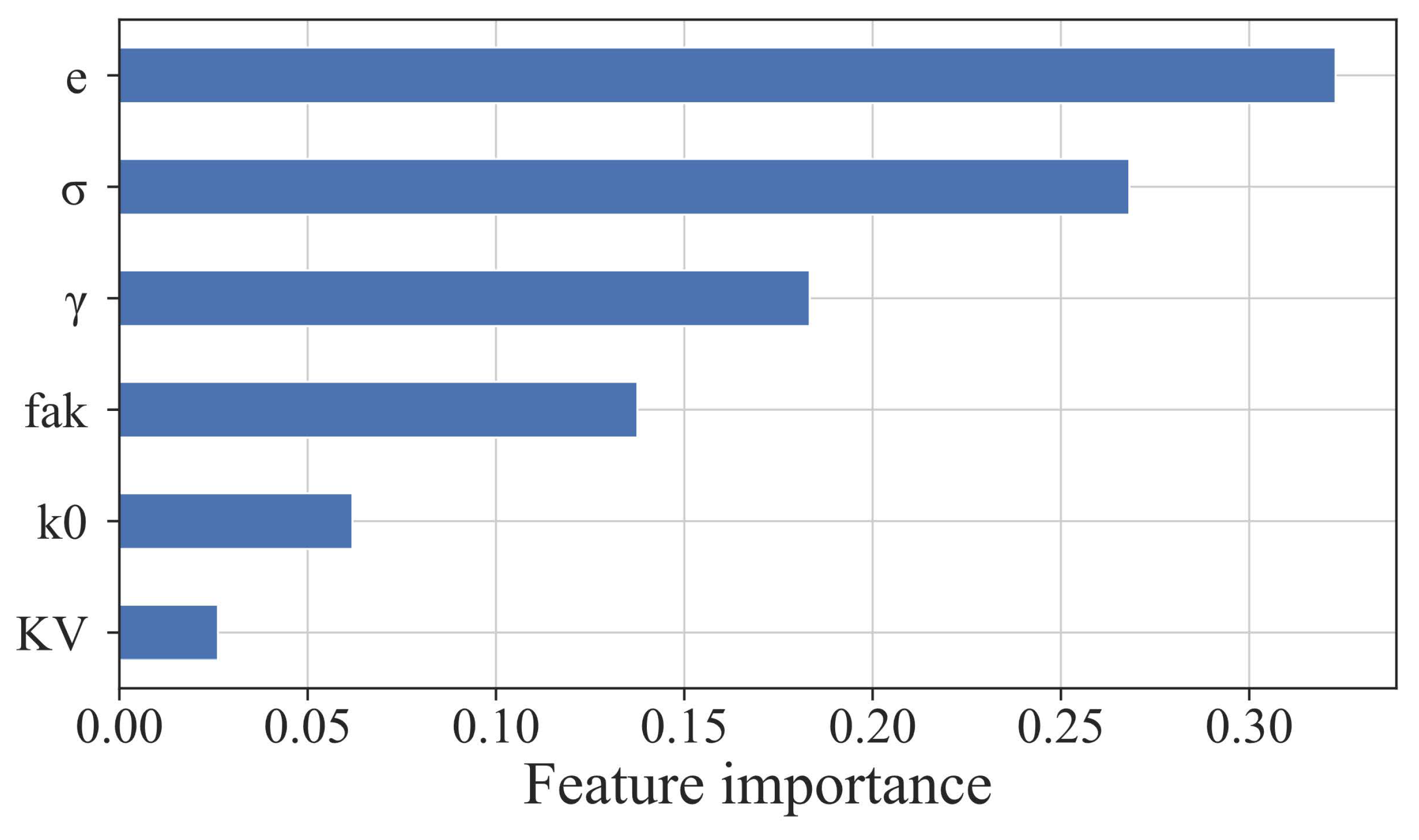
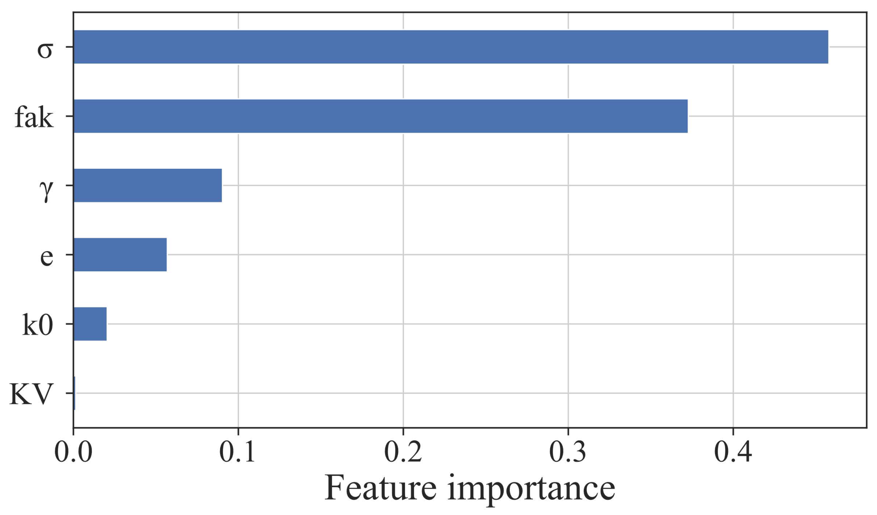
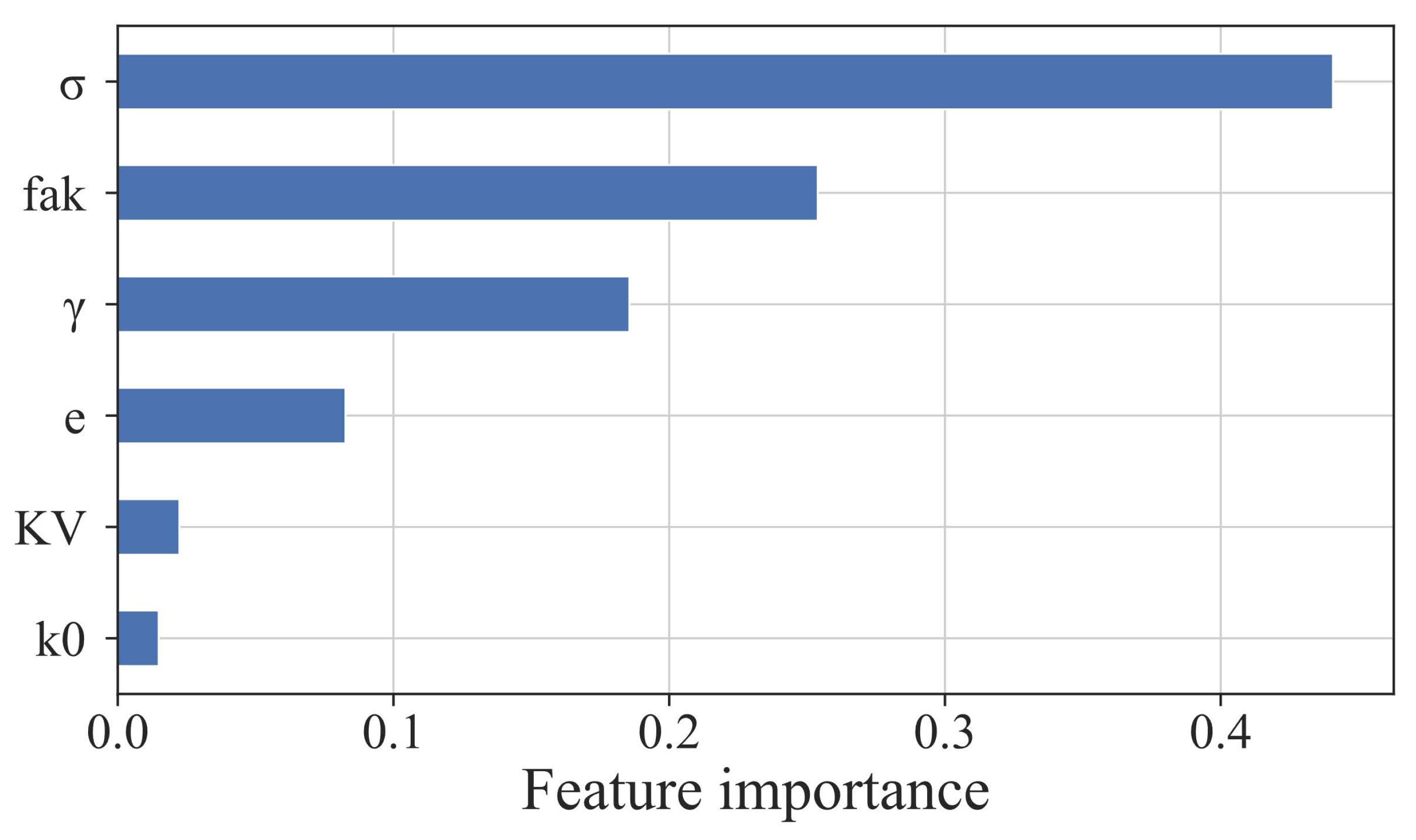
4.1. Feature Importance of Geotechnical Parameters for Consumption Factors

The training dataset for random forest method is crucial to its prediction accuracy. Consequently, the pre-processing described in the previous section is necessary for the dataset before analysis. 6 parameters of different geological layers are taken into account in variable importance analysis for main consumption factors (greases, grouting, labor, electricity and water) in this subsection.

The strategy of the data preparation are arranged as follows. The reduced input dataset contains 6 geotechnical parameters: natural density, void ratio, bearing capacity, lateral pressure coefficient, vertical permeability coefficient and compressive strength. The objective parameter is set as the concerned factors, and they will be analyzed one by one in the established random forest model. Arranged in the order of the shield segment index, 1979 sets containing above 6 parameters in different geological conditions are derived as the dataset of the model. Among them, 1485 (75%) sets are used as the training set of random forest model, and 494 (25%) sets will be predicted by the trained model (test set) and compared to the true values, aiming at validating the prediction accuracy.

The direct use of original data may result in accuracy issues caused by the dominance of large dimension values, as the input and output data of the model have different units and can fluctuate substantially in value. As the model training process uses gradient descent optimization, the difference in dimensions can slow down the rate at which model parameters are updated in each iteration. To prevent these issues, we normalize the input and output data during the preprocessing step and scale them linearly to the interval of $[0,1]$ using Equation (10). This normalization and scaling procedure ensures that the model is not affected by differences in data dimensions.

$$x^{*}=\frac{x-x_{\min }}{x_{\max }-x_{\min }}$$

(10)

where x denotes the original input and output data values, $x_{m}in$ and $x_{m}ax$ are the minimum and maximum values, and $x^{*}$ is the objective normalized value that can be employed in the proposed model.

The suggested random forest model has been trained using the aforementioned stages, taking various model parameters into consideration (criterion, number of estimators, minimum samples leaf and split). The ideal answer can be found by comparing the forecast accuracy with various structures. Different numbers of estimators (50, 100, 400, 700, 1000) with 1, 5, 10, 15, 20 minimum samples leaves and 2, 4, 10, 12, 16 minimum samples splits have been attempted.

Inspired by Santos et al. [47], we have plotted the six geological parameters and the quantity of material consumption in the same order of shield segment in Figure 11 and Figure 12. To avoid repetition, we will only discuss tail grease (red curve in Figure 11) and grouting (purple curve in Figure 12). The values of the geological parameters have been normalized using Equation (10). It is observed that the different geological conditions in the excavation area can be reflected by the variation of geological parameters, and there is a correlation with material consumption. However, the most important geological feature and exact relation cannot be directly seen and need to be analyzed using the constructed random forest model.

For the sake of clarity, the final value of the best score at the end of the training process and calculation efficiency of different random forest structures are illustrated in Figure 13 (the criterion Gini is always chosen by the program instead of Entropy). It can be concluded in Figure 13a that except for 400 and 700, the final value of the best score does not have remarkable changes with the variation of the number of estimators, where it takes the maximum value with 50. Besides, as shown in Figure 13b,c, the values of accuracy levels are all acceptable for different numbers of the minimum samples leaf and samples split. Consequently, considering the best performance, the random forest model with 50 estimators with one minimum samples leaves and two samples splits was adopted for the training and prediction steps. The final accuracy level (best score) of the test data is 0.9403.

With the above set of model parameters, the importance of each geotechnical feature is firstly calculated in the random forest model for the consumption factor grease (tail grease, EP2 grease and seal grease). The obtained results are shown in Figure 14, with the vertical axis being the geotechnical features and the horizontal axis being the magnitude of corresponding importance. It can be seen from the three subfigures that the compressive strength ($\mathsf{\sigma }$) of material has the most important impact on the prediction of all the three types of greases. More precisely, the strength parameter exhibits obviously the greatest importance than other geotechnical parameters for consumption of tail grease (first subfigure of Figure 14), where the correlation is more than 48%. While for seal grease (third subfigures), the most significant geotechnical parameter is also the strength, the difference with the second parameter is not that much greater than that in the first one (the following important feature is a void ratio). Notice for the EP2 grease, for the strength in the second impactful geotechnical feature, the difference with the first one (fak) is not great. Consequently, the strength can be concluded as the most impactful geotechnical parameter on the consumption of greases in general. The accuracy levels for Figure 14 are 0.9413, 0.9357 and 0.9608, respectively.

Figure 15, Figure 16, Figure 17 and Figure 18 display the geotechnical feature importance for the consumption of grouting, labor and electricity and water in shield tunneling, respectively. Similar to the variable importance analysis of grease, the most impactful geotechnical parameter for the consumption of grouting and labor is also the strength of material, obviously (see Figure 16 and Figure 18). The accuracy levels are 0.893, 0.7333, 0.9317 and 0.9252, respectively.

On the contrary, concerning the consumption of grouting, the most important geotechnical parameter is obtained as the void ratio ($\mathrm{e}$) of the material, instead of the strength (Figure 15), which is in second place. The corresponding importance is 0.27. It is reasonable that the grouting quantity is related to the void ratio of the material from the point of view of geomechanics, because large porosity will lead to more backfill grouting in shield tunneling. As a result, the strength of soil or rock is not the most important feature for all the considered consumption factors. In order to find a single geotechnical parameter for the classification of the quota of budget in complex geological conditions, more computation of the total cost is needed to verify the selected feature, verifying if it can be used as the classification index in general. This will be provided in the next subsection.

In addition, for the purposes of evaluation of the prediction by random forest model, the confusion matrix for each target consumption factor was also carried out. The confusion matrix displays predictions that are both correct and incorrect, and the results are evaluated in light of the actual values. The confusion matrix can show how the random forest classification model gets confused while making predictions. The four values in the matrix are True Positive (TP), False Positive (FP), False Negative (FN), and True Negative (TN), respectively. Thus, the accuracy levels for each target can be calculated as:

$$\mathrm{AC}=\frac{\mathrm{TP}+\mathrm{TN}}{\mathrm{TP}+\mathrm{FP}+\mathrm{FN}+\mathrm{TN}}.$$

(11)

In Figure 19, the number of correct predictions and the number of incorrect predictions for tail grease are displayed in two subfigures (left: training set; right: test set), respectively. Consequently, the accuracy levels for calculating the variable importance can also be obtained by Equation (11). It is seen that the obtained results by the proposed model are reliable. In order to avoid repetition, the confusion matrix for other factors is not illustrated here.

4.2. Quota of Budget for Shield Tunneling in Complex Geological Conditions Based on the Random Forest Results

In this part, we aim at establishing a quota budget for shield tunneling in complex geological conditions based on the random forest results obtained in the previous subsection. From the above computation, the compressive strength ($\mathsf{\sigma }$) is the most important feature for the consumption of grease, labor and electricity and water, while it is the second influencing geotechnical parameter for grouting (the most impactful parameter is the void ratio). For the sake of simplicity in engineering, it is supposed to consider only one geotechnical parameter to produce the classification in the quota of budgets in complex conditions. As a result, we assume that all the considered economic factors can be classified by the compressive strength index. We will also verify the prediction accuracy by comparing the total cost computed by the constructed model with that defined by the available quota.

Inspired by the classification standard for the engineering rock mass and code for geotechnical engineering investigation of China, let us introduce the following classification based on the compressive strength of geomaterials, as shown in

Table 3. Classification of engineering geomaterials by compressive strength.

Type	Compressive Strength (MPa)
Soil	≤1
Soft rock	≤30
Hard rock	≥30

. Consequently, we propose a classification with three categories (hard rock, soft rock and soil) by identifying the compressive strength, and continue the analysis.

The collected data of the concerned consumption in shield tunneling have been reclassified by the compressive strength as in Table 3, so all the consumption data for grease, grouting, labor and electricity and water are recounted in the above three categories. The obtained average values for each category with respect to tunneling consumption are displayed in

Table 4. Comparison of main consumption and cost in different geological conditions with the standard values.

Factor	Quota	Soil		Soft Rock		Hard Rock
Tail grease	81.90	70.50	118%	84.99	136%	145.88	399%
EP2 grease		14.18		14.16		70.79
Seal grease		12.72		12.58		110.46
Grouting	1.3–1.8	1.49		1.60		2.12
Labor	51.73	51.34	99%	61.90	120%	106.24	205%
Water	78.93	176.74	223%	227.92	289%	334.65	424%
Electricity	10,800	7449.25	69%	9565	89%	25,885	239%
Total cost	72,153	68,039	94%	72,996	101%	99,719	138%

Only the concerned consumption (part of the main materials and labor) have been listed in this Table, other materials and machine-teams which remain the same have not been listed, but included in the total cost.

. The standard value defined by the available official quota is also provided in the same table for comparison (per meter). In general, the considered consumption quantities exhibit an obvious positive correlation with the compressive strength of geomaterial. It can be seen that the consumption per meter in shield tunneling is increasing from soil to hard rock, also for the grouting quantity.

To elaborate, for soft rock and soil, the differences of main consumption are not as great as that between soft rock and hard rock. Consequently, the construction cost of shield tunneling is much more expensive, which is consistent with the actual situation. This proves the rationality of the classification for the quota from the side. Comparing with the standard values, the obtained results in soil are slightly smaller, while those in soft rock are close to the standard quantities. Concerning the consumption of hard rock, all the tunneling consumption is obviously greater than the standard value, even greater than two times. Consequently, for the tunneling project in complex geological conditions, the total budget cannot be calculated accurately by the present standard quota. It must be pointed out that only the concerned varying consumption has been listed in Table 4, other materials and machine-teams which remain the same have been not listed, but included in the total cost.

The total cost of the tunneling project per meter is provided in Figure 20. The cost for each factor can be calculated by the use of the values in Table 4, and the total cost can be obtained by accumulating the components. It is seen that the total cost in tunneling also has an evident positive correlation with the compressive strength, increasing from soil to hard rock. Although the most impactful geotechnical feature for grouting is not the strength (because the most impactful geotechnical parameter is a void ratio), the strength can still be used for defining the new quota of budgets in complex geological conditions. The total cost for soft rock is close to the original budget of the shield tunneling project, while that for soil is 6% lower than the standard cost. What is more, the total cost for hard rock is 38% higher than the standard cost, which cannot be ignored in complex conditions. This is the most important remark of this study, that the compressive strength can be chosen as the classification index, and the proposed categories in Table 3 are an effective reference scheme.

It must be pointed out by recent research that the random forest model can have limited extrapolation ability, and it may not perform well when applied to data that fall outside the range of the training set [48,49]. However, the main objective of our study was to determine the most influential geological parameter for material consumption in shield tunneling. In this context, the random forest algorithm is suitable for determining feature importance. Besides, increasing the size of datasets can help random forest models capture more patterns in the data, which we have done in our study by collecting geological parameters from soft soil to hard rock. Additionally, we have carefully selected the hyperparameters of the random forest model to optimize its performance and improve its ability, as explained in the previous section. These efforts have helped us to mitigate the limitation of extrapolation in the random forest model to a certain extent. Moreover, due to the limitation of data sources, the constructed model was trained with the data collected from a single project, which may lead to inaccuracy if applied to other projects with varying geometric parameters. This needs to be improved in further research by collecting more data from different projects.

On the other hand, according to recent studies on Bayesian neural networks [50,51], the strong spatial variability of soil properties can affect the accuracy of deterministic data-driven models. Thus, deterministic data-driven models may incur large errors and its prediction results cannot be evaluated. Advanced developments need to be taken into account in incorporating uncertainty to enhance the robustness of the proposed model, such as exploring the possibility of incorporating probabilistic models or stochastic techniques to account for the inherent variability and uncertainty of soil properties. This could potentially improve the reliability and accuracy of our model in predicting the material consumption in shield tunneling under various geological conditions.

5. Conclusions

In this study, we have proposed a random forest-based machine learning procedure to analyze the construction cost of shield tunneling in complex geological conditions. We identified the unit consumption of grease, grouting, labor, and water and electricity as the main factors affecting construction cost, based on engineering practice and expert opinions. To improve the accuracy of the model, we replenished empty and abnormal values in the input datasets and reduced its dimensionality from 17 to 6 using KNN and correlation analysis.

The proposed machine learning model was applied to the ZRT shield tunneling project and found that the compressive strength of geomaterial was the most influential geotechnical parameter for grease, labor, water, and electricity consumption. The consumption of grouting was mostly impacted by the void ratio, with compressive strength in second place. Based on these findings, we calculated and classified the unit consumption and cost of the ZRT tunneling project for three geological categories: soil, soft rock, and hard rock. Comparison with the standard value given by the official quota revealed that the unit cost of shield tunneling in soil was slightly lower (6%) than the standard cost, while that in soft rock was very close to the standard value. However, the cost in hard rock regions was significantly greater (38%) and cannot be ignored in budgeting. Thus, we recommend using the compressive strength as the classification index for shield tunneling in complex geological conditions.

In the outlook, collecting more data from different projects with varying tunnel diameters is an essential task in the future to improve the generalizability of the proposed model. Another interesting topic is to take into account advanced developments in incorporating uncertainty to enhance the robustness of the proposed model.

References

1. Demirkesen, S.; Ozorhon, B. Impact of integration management on construction project management performance. Int. J. Proj. Manag. 2017, 35, 1639–1654. [Google Scholar] [CrossRef]
2. Kim, S.; Chang, S.; Castro-Lacouture, D. Dynamic modeling for analyzing impacts of skilled labor shortage on construction project management. J. Manag. Eng. 2020, 36, 04019035. [Google Scholar] [CrossRef]
3. Kim, Y.; Bruland, A. A study on the establishment of Tunnel Contour Quality Index considering construction cost. Tunn. Undergr. Space Technol. 2015, 50, 218–225. [Google Scholar] [CrossRef]
4. Huang, Z.; Zhang, D.; Pitilakis, K.; Tsinidis, G.; Huang, H.; Zhang, D.; Argyroudis, S. Resilience assessment of tunnels: Framework and application for tunnels in alluvial deposits exposed to seismic hazard. Soil Dyn. Earthq. Eng. 2022, 162, 107456. [Google Scholar] [CrossRef]
5. Mesároš, P.; Mandičák, T. Exploitation and benefits of BIM in construction project management. IOP Conf. Ser. Mater. Sci. Eng. 2017, 245, 062056. [Google Scholar] [CrossRef] [Green Version]
6. Chmelina, K.; Rabensteiner, K.; Krusche, G. A tunnel information system for the management and utilization of geo-engineering data in urban tunnel projects. Geotech. Geol. Eng. 2013, 31, 845–859. [Google Scholar] [CrossRef]
7. Li, J.; Jing, L.; Zheng, X.; Li, P.; Yang, C. Application and outlook of information and intelligence technology for safe and efficient TBM construction. Tunn. Undergr. Space Technol. 2019, 93, 103097. [Google Scholar] [CrossRef]
8. Vargas, J.P.; Koppe, J.C.; Pérez, S.; Hurtado, J.P. Planning tunnel construction using Markov chain Monte Carlo (MCMC). Math. Probl. Eng. 2015, 797953. [Google Scholar] [CrossRef] [Green Version]
9. Park, J.; Lee, K.H.; Park, J.; Choi, H.; Lee, I.M. Predicting anomalous zone ahead of tunnel face utilizing electrical resistivity: I. Algorithm and measuring system development. Tunn. Undergr. Space Technol. 2016, 60, 141–150. [Google Scholar] [CrossRef]
10. Park, J.; Lee, K.H.; Kim, B.K.; Choi, H.; Lee, I.M. Predicting anomalous zone ahead of tunnel face utilizing electrical resistivity: II. Field tests. Tunn. Undergr. Space Technol. 2017, 68, 1–10. [Google Scholar] [CrossRef]
11. Leu, S.S.; Joko, T.; Sutanto, A. Applied real-time Bayesian analysis in forecasting tunnel geological conditions. In Proceedings of the 2010 IEEE International Conference on Industrial Engineering and Engineering Management, Macao, China, 7–10 December 2010; pp. 1505–1508. [Google Scholar]
12. Mahmoodzadeh, A.; Zare, S. Probabilistic prediction of expected ground condition and construction time and costs in road tunnels. J. Rock Mech. Geotech. Eng. 2016, 8, 734–745. [Google Scholar] [CrossRef]
13. Lee, J.; Sagong, M.; Cho, G.C.; Choo, S. Experimental estimation of the fallout size and reinforcement design of a tunnel under excavation. Tunn. Undergr. Space Technol. 2010, 25, 518–525. [Google Scholar] [CrossRef]
14. Guan, Z.; Deng, T.; Jiang, Y.; Zhao, C.; Huang, H. Probabilistic estimation of ground condition and construction cost for mountain tunnels. Tunn. Undergr. Space Technol. 2014, 42, 175–183. [Google Scholar] [CrossRef]
15. Zhang, Q.; Liu, Z.; Tan, J. Prediction of geological conditions for a tunnel boring machine using big operational data. Autom. Constr. 2019, 100, 73–83. [Google Scholar] [CrossRef]
16. Carrière, S.D.; Chalikakis, K.; Sénéchal, G.; Danquigny, C.; Emblanch, C. Combining electrical resistivity tomography and ground penetrating radar to study geological structuring of karst unsaturated zone. J. Appl. Geophys. 2013, 94, 31–41. [Google Scholar] [CrossRef]
17. Daraei, A.; H Sherwani, A.F.; Faraj, R.H.; Kalhor, Q.; Zare, S.; Mahmoodzadeh, A. Optimization of the outlet portal of Heybat Sultan twin tunnels based on the value engineering methodology. SN Appl. Sci. 2019, 1, 1–10. [Google Scholar] [CrossRef] [Green Version]
18. Mahmoodzadeh, A.; Mohammadi, M.; Abdulhamid, S.N.; Nejati, H.R.; Noori, K.M.G.; Ibrahim, H.H.; Ali, H.F.H. Predicting construction time and cost of tunnels using Markov chain model considering opinions of experts. Tunn. Undergr. Space Technol. 2021, 116, 104109. [Google Scholar] [CrossRef]
19. Shi, L.; Zhang, J.; Zhu, Q.; Sun, H. Prediction of mechanical behavior of rocks with strong strain-softening effects by a deep-learning approach. Comput. Geotech. 2022, 152, 105040. [Google Scholar] [CrossRef]
20. Mahmoodzadeh, A.; Mohammadi, M.; Daraei, A.; Farid Hama Ali, H.; Ismail Abdullah, A.; Kameran Al-Salihi, N. Forecasting tunnel geology, construction time and costs using machine learning methods. Neural Comput. Appl. 2021, 33, 321–348. [Google Scholar] [CrossRef]
21. Ye, D. An Algorithm for Construction Project Cost Forecast Based on Particle Swarm Optimization-Guided BP Neural Network. Sci. Program. 2021, 2021, 4309495. [Google Scholar] [CrossRef]
22. Lin, T.; Yi, T.; Zhang, C.; Liu, J. Intelligent prediction of the construction cost of substation projects using support vector machine optimized by particle swarm optimization. Math. Probl. Eng. 2019, 7631362. [Google Scholar] [CrossRef]
23. Liu, J.B.; Ren, H.; Li, Z.M. Model on dynamic control of project costs based on GM (1, 1) for construction enterprises. In Fuzzy Information and Engineering Volume 2; Springer: Berlin/Heidelberg, Germany, 2009; pp. 1611–1620. [Google Scholar]
24. Min, S.; Einstein, H.; Lee, J.; Kim, T. Application of decision aids for tunneling (DAT) to a drill & blast tunnel. KSCE J. Civ. Eng. 2003, 7, 619–628. [Google Scholar]
25. Maruvanchery, V.; Zhe, S.; Robert, T.L.K. Early construction cost and time risk assessment and evaluation of large-scale underground cavern construction projects in Singapore. Undergr. Space 2020, 5, 53–70. [Google Scholar] [CrossRef]
26. Shi, S.S.; Li, S.C.; Li, L.P.; Zhou, Z.Q.; Wang, J. Advance optimized classification and application of surrounding rock based on fuzzy analytic hierarchy process and Tunnel Seismic Prediction. Autom. Constr. 2014, 37, 217–222. [Google Scholar] [CrossRef]
27. Belgiu, M.; Drăguţ, L. Random forest in remote sensing: A review of applications and future directions. ISPRS J. Photogramm. Remote Sens. 2016, 114, 24–31. [Google Scholar] [CrossRef]
28. Feng, X.; Jimenez, R. Predicting tunnel squeezing with incomplete data using Bayesian networks. Eng. Geol. 2015, 195, 214–224. [Google Scholar] [CrossRef]
29. Zhang, P.; Yin, Z.Y.; Jin, Y.F. Machine learning-based modelling of soil properties for geotechnical design: Review, tool development and comparison. Arch. Comput. Methods Eng. 2022, 29, 1229–1245. [Google Scholar] [CrossRef]
30. Lu, L.; Meng, X.; Mao, Z.; Karniadakis, G.E. DeepXDE: A deep learning library for solving differential equations. SIAM Rev. 2021, 63, 208–228. [Google Scholar] [CrossRef]
31. Ho, T.K. Random decision forests. In Proceedings of the 3rd International Conference on Document Analysis and Recognition, Montreal, QC, Canada, 14–16 August 1995; Volume 1, pp. 278–282. [Google Scholar]
32. Ho, T.K. The random subspace method for constructing decision forests. IEEE Trans. Pattern Anal. Mach. Intell. 1998, 20, 832–844. [Google Scholar]
33. Breiman, L. Random forests. Mach. Learn. 2001, 45, 5–32. [Google Scholar] [CrossRef] [Green Version]
34. Strobl, C.; Boulesteix, A.L.; Augustin, T. Unbiased split selection for classification trees based on the Gini index. Comput. Stat. Data Anal. 2007, 52, 483–501. [Google Scholar] [CrossRef] [Green Version]
35. Palomino, A.F.; Espino, P.S.; Reyes, C.B.; Rojas, J.A.J.; y Silva, F.R. Estimation of moisture in live fuels in the mediterranean: Linear regressions and random forests. J. Environ. Manag. 2022, 322, 116069. [Google Scholar] [CrossRef] [PubMed]
36. Smith, P.F.; Ganesh, S.; Liu, P. A comparison of random forest regression and multiple linear regression for prediction in neuroscience. J. Neurosci. Methods 2013, 220, 85–91. [Google Scholar] [CrossRef] [PubMed]
37. Piryonesi, S.M. The Application of Data Analytics to Asset Management: Deterioration and Climate Change Adaptation in Ontario Roads. Ph.D. Thesis, University of Toronto, Toronto, ON, Canada, 2019. [Google Scholar]
38. Rajković, D.; Jeromela, A.M.; Pezo, L.; Lončar, B.; Grahovac, N.; Špika, A.K. Artificial neural network and random forest regression models for modelling fatty acid and tocopherol content in oil of winter rapeseed. J. Food Compos. Anal. 2023, 115, 105020. [Google Scholar] [CrossRef]
39. Kang, K.; Ryu, H. Predicting types of occupational accidents at construction sites in Korea using random forest model. Saf. Sci. 2019, 120, 226–236. [Google Scholar] [CrossRef]
40. Tixier, A.J.P.; Hallowell, M.R.; Rajagopalan, B.; Bowman, D. Application of machine learning to construction injury prediction. Autom. Constr. 2016, 69, 102–114. [Google Scholar] [CrossRef] [Green Version]
41. Wang, L.; Mao, Z.; Xuan, H.; Ma, T.; Hu, C.; Chen, J.; You, X. Status diagnosis and feature tracing of the natural gas pipeline weld based on improved random forest model. Int. J. Press. Vessel. Pip. 2022, 200, 104821. [Google Scholar] [CrossRef]
42. Gu, Y.; Liu, D.; Arvin, R.; Khattak, A.J.; Han, L.D. Predicting intersection crash frequency using connected vehicle data: A framework for geographical random forest. Accid. Anal. Prev. 2023, 179, 106880. [Google Scholar] [CrossRef]
43. Zermane, A.; Tohir, M.Z.M.; Zermane, H.; Baharudin, M.R.; Yusoff, H.M. Predicting fatal fall from heights accidents using random forest classification machine learning model. Saf. Sci. 2023, 159, 106023. [Google Scholar] [CrossRef]
44. Mishra, N.B.; Crews, K.A. Mapping vegetation morphology types in a dry savanna ecosystem: Integrating hierarchical object-based image analysis with Random Forest. Int. J. Remote Sens. 2014, 35, 1175–1198. [Google Scholar] [CrossRef]
45. Guan, H.; Li, J.; Chapman, M.; Deng, F.; Ji, Z.; Yang, X. Integration of orthoimagery and lidar data for object-based urban thematic mapping using random forests. Int. J. Remote Sens. 2013, 34, 5166–5186. [Google Scholar] [CrossRef]
46. Peterson, L.E. K-nearest neighbor. Scholarpedia 2009, 4, 1883. [Google Scholar] [CrossRef]
47. Santos, O.J., Jr.; Celestino, T.B. Artificial neural networks analysis of Sao Paulo subway tunnel settlement data. Tunn. Undergr. Space Technol. 2008, 23, 481–491. [Google Scholar] [CrossRef]
48. Takoutsing, B.; Heuvelink, G.B. Comparing the prediction performance, uncertainty quantification and extrapolation potential of regression kriging and random forest while accounting for soil measurement errors. Geoderma 2022, 428, 116192. [Google Scholar] [CrossRef]
49. Carrasco, L.; Toquenaga, Y.; Mashiko, M. Extrapolation of random forest models shows scale adaptation in egret colony site selection against landscape complexity. Ecol. Complex. 2015, 24, 29–36. [Google Scholar] [CrossRef]
50. Yang, L.; Meng, X.; Karniadakis, G.E. B-PINNs: Bayesian physics-informed neural networks for forward and inverse PDE problems with noisy data. J. Comput. Phys. 2021, 425, 109913. [Google Scholar] [CrossRef]
51. Zhang, P.; Yin, Z.Y.; Jin, Y.F. Bayesian neural network-based uncertainty modelling: Application to soil compressibility and undrained shear strength prediction. Can. Geotech. J. 2022, 59, 546–557. [Google Scholar] [CrossRef]
Figure 1. The background and location of the Zhijiang Road Tunneling (ZRT) project in Hangzhou, China.
Mathematics 11 01423 g001
Figure 2. Main geological compositions of west (above) and east (below) sections of shield tunneling excavation in ZRT project.
Mathematics 11 01423 g002
Figure 3. Profile of main geological conditions along the east tunnel.
Mathematics 11 01423 g003
Figure 4. Shield segments index.
Mathematics 11 01423 g004
Figure 5. Missing values of all 17 geotechnical parameters arranged in the order of shield segment.
Mathematics 11 01423 g005
Figure 6. Distribution of original data and that treated by the KNN algorithm of compressive strength ( σ ) (left subfigure) and void ratio ( e ) (right subfigure).
Mathematics 11 01423 g006
Figure 7. Correlation matrix heat map of nine geological parameters.
Mathematics 11 01423 g007
Figure 8. Final six geotechnical features in random forest model by dimension reduction.
Mathematics 11 01423 g008
Figure 9. Expansion of Random Forest structure.
Mathematics 11 01423 g009
Figure 10. Flowchart of analysis on main consumption factors of shield tunneling in complex geological conditions by random forest algorithm.
Mathematics 11 01423 g010
Figure 11. Collected geological parameters and tail grease in the order of shield segment.
Mathematics 11 01423 g011
Figure 12. Collected geological parameters and grouting in the order of shield segment.
Mathematics 11 01423 g012
Figure 13. Comparison of the best score with different random forest structures.
Mathematics 11 01423 g013
Figure 14. Variable importance for tail grease, EP2 grease and seal grease by random forest model in shield tunneling.
Mathematics 11 01423 g014
Figure 15. Variable importance for grouting quantity by random forest model in shield tunneling.
Mathematics 11 01423 g015
Figure 16. Variable importance for labor by random forest model in shield tunneling.
Mathematics 11 01423 g016
Figure 17. Variable importance for water consumption by random forest model in shield tunneling.
Mathematics 11 01423 g017
Figure 18. Variable importance for electricity consumption by random forest model in shield tunneling.
Mathematics 11 01423 g018
Figure 19. Confusion matrix for the consumption of tail grease (left: training set; right: test set).
Mathematics 11 01423 g019
Figure 20. Comparison of unit cost of standard quota and by random forest algorithm for different geological conditions (Currency: CNY).
Mathematics 11 01423 g020