
Effect of Impaired B-Cell and CTL Functions on HIV-1 Dynamics

Abstract
:1. Introduction
2. HIV-1 Model with Impaired B-Cell and CTL Functions
2.1. Model Description
2.2. Model Analysis
2.2.1. Properties of Solutions
2.2.2. Reproductive Number and Steady States
- (i)
- The system always has an infection-free steady state (); and
- (ii)
- If , the system also has an infected steady state ().
2.2.3. Stability of Steady States and
2.3. Comparison of Results
3. Model with Distributed Time Delays
3.1. Model Description
3.2. Model Analysis
3.2.1. Basic Properties of Solutions
3.2.2. Reproduction Number and Steady States
- (i)
- The system always has an infection-free steady state (); and
- (ii)
- If , the system also has an infected steady state ().
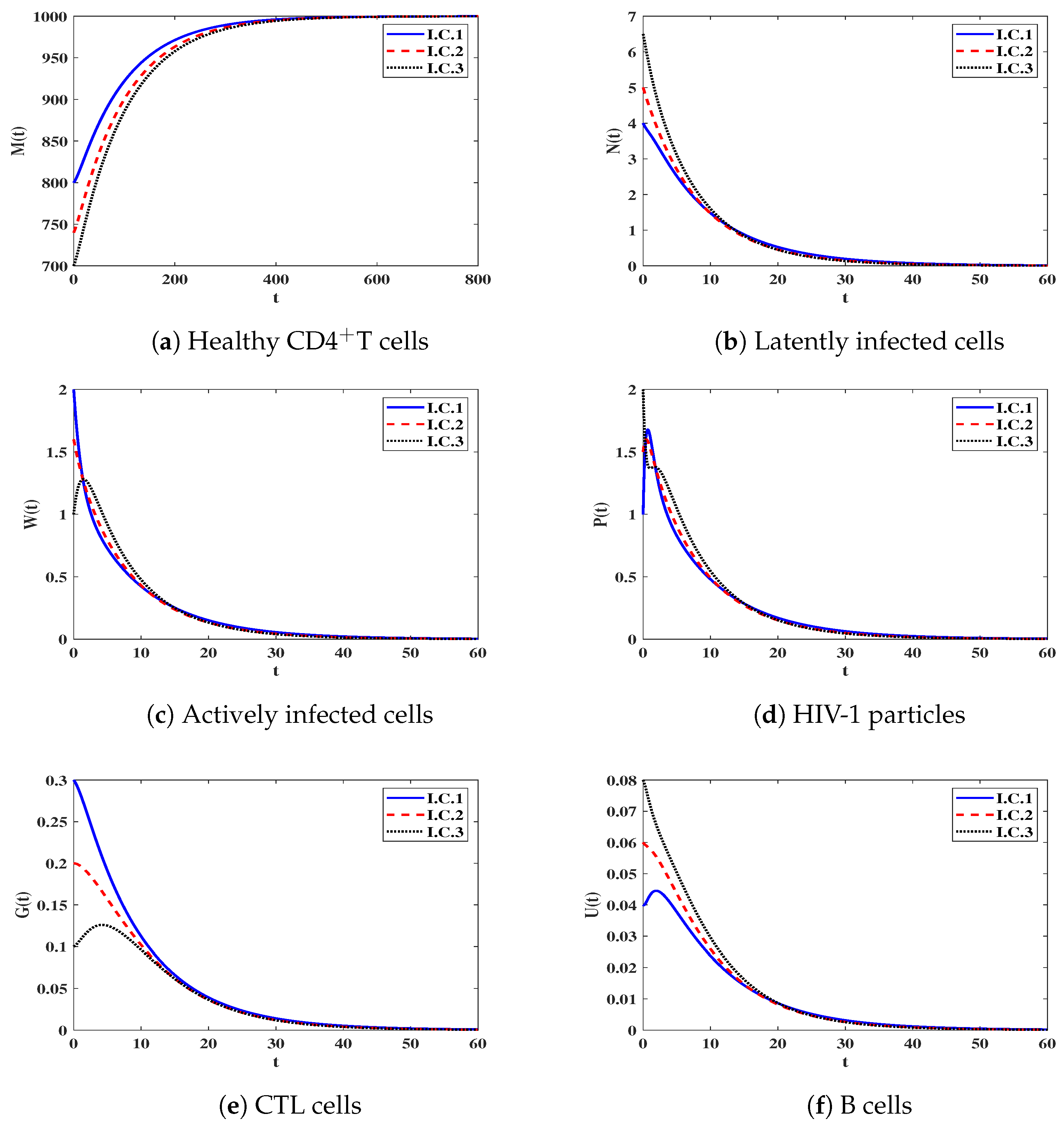
3.2.3. Stability of Steady States and
3.3. Numerical Simulation for Model (12)
3.3.1. Effect of and on Stability of Steady States
3.3.2. Effect of Impaired CTLs and B-Cells
3.4. Numerical Simulation for Model (17)
Impact of Time Delays on Stability of Steady States
- We solve system (19) under the following initial condition:
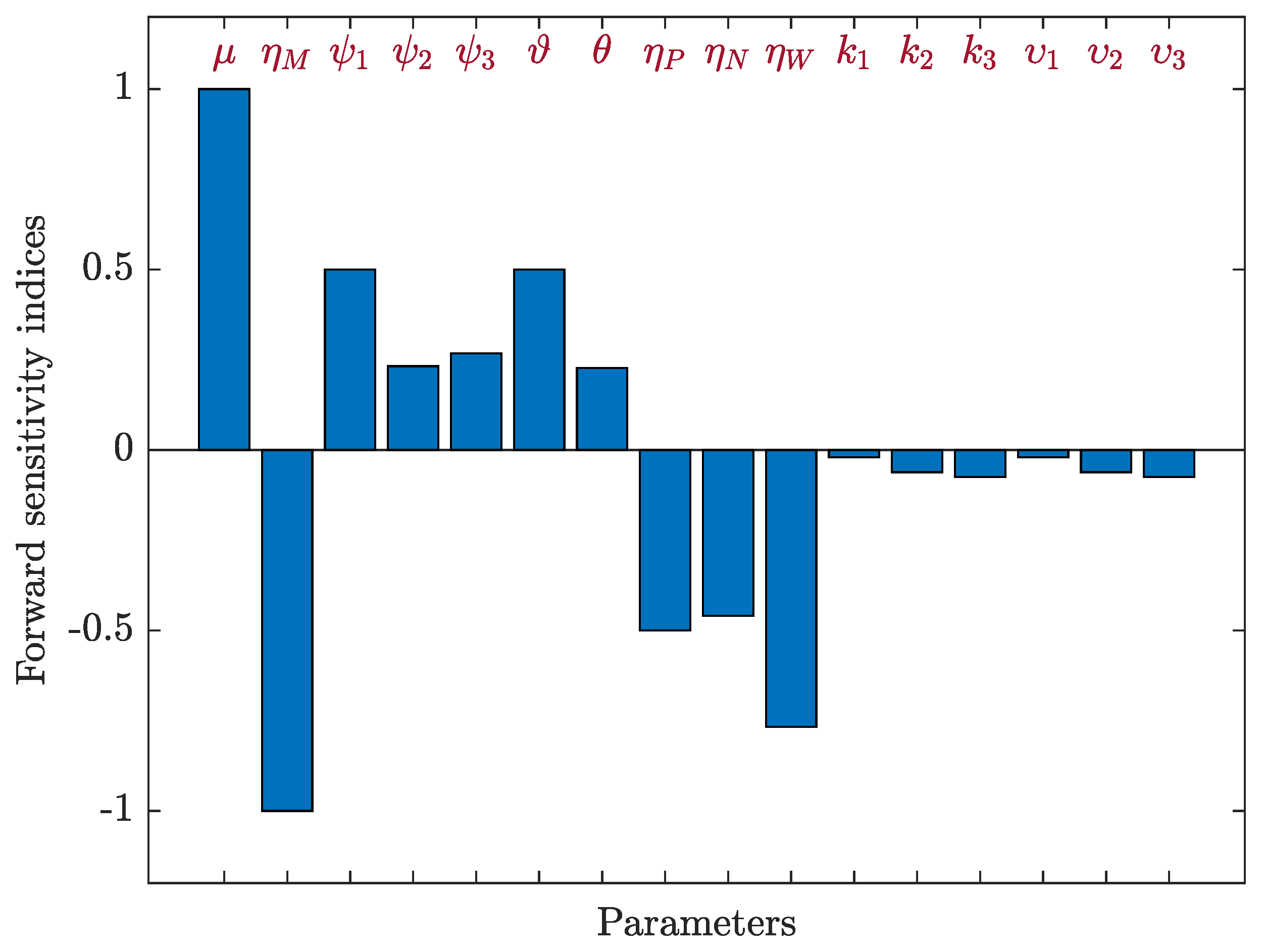
3.5. Sensitivity Analysis
3.5.1. Sensitivity Analysis for Model (12)
3.5.2. Sensitivity Analysis for Model (19)
4. Conclusions and Discussion
Future Works
- Modify the model by adding the diffusion of all compartments as:where is the position, and is the diffusion coefficient of compartment u.
- Using real data to estimate the model’s parameters;
- Considering the age structure in the infected cells;
- Considering viral mutations.
Author Contributions
Funding
Data Availability Statement
Acknowledgments
Conflicts of Interest
Appendix A
- , which yields the infection-free steady state ().
- and . Let be a function on the interval , defined as:
- , which leads to the infection-free steady state ;
- and . Let be a function of interval , defined as:
References
- Wodarz, D.; Levy, D.N. Human immunodeficiency virus evolution towards reduced replicative fitness in vivo and the development of AIDS. Proc. R. Soc. Biol. Sci. 2007, 274, 2481–2491. [Google Scholar] [CrossRef]
- Available online: https://www.who.int/data/gho/data/themes/hiv-aids (accessed on 1 September 2023).
- Nowak, M.A.; Bangham, C.R.M. Population dynamics of immune responses to persistent viruses. Science 1996, 272, 74–79. [Google Scholar] [CrossRef]
- Nowak, M.A.; May, R.M. Virus Dynamics; Oxford University Press: New York, NY, USA, 2000. [Google Scholar]
- Lv, C.; Huang, L.; Yuan, Z. Global stability for an HIV-1 infection model with Beddington-DeAngelis incidence rate and CTL immune response. Commun. Nonlinear Sci. Numer. Simul. 2014, 19, 121–127. [Google Scholar] [CrossRef]
- Jiang, C.; Kong, H.; Zhang, G.; Wang, K. Global properties of a virus dynamics model with self-proliferation of CTLs. Math. Appl. Sci. Eng. 2021, 2, 123–133. [Google Scholar] [CrossRef]
- Ren, J.; Xu, R.; Li, L. Global stability of an HIV infection model with saturated CTL immune response and intracellular delay. Math. Biosci. Eng. 2020, 18, 57–68. [Google Scholar] [CrossRef] [PubMed]
- Wang, A.P.; Li, M.Y. Viral dynamics of HIV-1 with CTL immune response. Discret. Contin. Dyn. Syst. Ser. B 2021, 26, 2257–2272. [Google Scholar] [CrossRef]
- Yang, Y.; Xu, R. Mathematical analysis of a delayed HIV infection model with saturated CTL immune response and immune impairment. J. Appl. Math. Comput. 2022, 68, 2365–2380. [Google Scholar] [CrossRef]
- Chen, C.; Zhou, Y. Dynamic analysis of HIV model with a general incidence, CTLs immune response and intracellular delays. Math. Comput. Simul. 2023, 212, 159–181. [Google Scholar] [CrossRef]
- Wodarz, D.; May, R.M.; Nowak, M.A. The role of antigen-independent persistence of memory cytotoxic T lymphocytes. Int. Immunol. 2000, 12, 467–477. [Google Scholar] [CrossRef]
- Elaiw, A.M.; AlShamrani, N.H. Global stability of humoral immunity virus dynamics models with nonlinear infection rate and removal. Nonlinear Anal. Real World Appl. 2015, 26, 161–190. [Google Scholar] [CrossRef]
- Wang, S.; Zou, D. Global stability of in host viral models with humoral immunity and intracellular delays. Appl. Math. Model. 2012, 36, 1313–1322. [Google Scholar] [CrossRef]
- Tang, S.; Teng, Z.; Miao, H. Global dynamics of a reaction–diffusion virus infection model with humoral immunity and nonlinear incidence. Comput. Math. Appl. 2019, 78, 786–806. [Google Scholar] [CrossRef]
- Zheng, T.; Luo, Y.; Teng, Z. Spatial dynamics of a viral infection model with immune response and nonlinear incidence. Z. Für Angew. Math. Und Phys. 2023, 74, 124. [Google Scholar] [CrossRef] [PubMed]
- Kajiwara, T.; Sasaki, T.; Otani, Y. Global stability for an age-structured multistrain virus dynamics model with humoral immunity. J. Appl. Math. Comput. 2020, 62, 239–279. [Google Scholar] [CrossRef]
- Dhar, M.; Samaddar, S.; Bhattacharya, P. Modeling the effect of non-cytolytic immune response on viral infection dynamics in the presence of humoral immunity. Nonlinear Dyn. 2019, 98, 637–655. [Google Scholar] [CrossRef]
- Murase, A.; Sasaki, T.; Kajiwara, T. Stability analysis of pathogen-immune interaction dynamics. J. Math. Biol. 2005, 51, 247–267. [Google Scholar] [CrossRef]
- Wodarz, D. Hepatitis C virus dynamics and pathology: The role of CTL and antibody responses. J. Gen. Virol. 2003, 84, 1743–1750. [Google Scholar] [CrossRef] [PubMed]
- Wang, J.; Pang, J.; Kuniya, T.; Enatsu, Y. Global threshold dynamics in a five-dimensional virus model with cell-mediated, humoral immune responses and distributed delays. Appl. Math. Comput. 2014, 241, 298–316. [Google Scholar] [CrossRef]
- Yan, Y.; Wang, W. Global stability of a five-dimensional model with immune responses and delay. Discret. Contin. Dyn. Syst. Ser. B 2012, 17, 401–416. [Google Scholar] [CrossRef]
- Dubey, P.; Dubey, U.S.; Dubey, B. Modeling the role of acquired immune response and antiretroviral therapy in the dynamics of HIV infection. Math. Comput. Simul. 2018, 144, 120–137. [Google Scholar] [CrossRef]
- Mondal, J.; Samui, P.; Chatterjee, A.N. Dynamical demeanour of SARS-CoV-2 virus undergoing immune response mechanism in COVID-19 pandemic. Eur. Phys. J. Spec. Top. 2022, 231, 3357–3370. [Google Scholar] [CrossRef]
- Sigal, A.; Kim, J.T.; Balazs, A.B.; Dekel, E.; Mayo, A.; Milo, R.; Baltimore, D. Cell-to-cell spread of HIV permits ongoing replication despite antiretroviral therapy. Nature 2011, 477, 95–98. [Google Scholar] [CrossRef]
- Martin, N.; Sattentau, Q. Cell-to-cell HIV-1 spread and its implications for immune evasion. Curr. Opin. HIV Aids 2009, 4, 143–149. [Google Scholar] [CrossRef] [PubMed]
- Dhar, M.; Samaddar, S.; Bhattacharya, P. Modeling the cell-to-cell transmission dynamics of viral infection under the exposure of non-cytolytic cure. J. Appl. Math. Comput. 2021, 65, 885–911. [Google Scholar] [CrossRef]
- Lin, J.; Xu, R.; Tian, X. Threshold dynamics of an HIV-1 virus model with both virus-to-cell and cell-to-cell transmissions, intracellular delay, and humoral immunity. Appl. Math. Comput. 2017, 315, 516–530. [Google Scholar] [CrossRef]
- Luo, Y.; Zhang, L.; Zheng, T.; Teng, Z. Analysis of a diffusive virus infection model with humoral immunity, cell-to-cell transmission and nonlinear incidence. Phys. A 2019, 535, 122415. [Google Scholar] [CrossRef]
- Wang, J.; Guo, M.; Liu, X.; Zhao, Z. Threshold dynamics of HIV-1 virus model with cell-to-cell transmission, cell-mediated immune responses and distributed delay. Appl. Math. Comput. 2016, 291, 149–161. [Google Scholar] [CrossRef]
- Cervantes-Perez, A.G.; Avila-Vales, E. Dynamical analysis of multipathways and multidelays of general virus dynamics model. Int. J. Bifurc. Chaos 2019, 29, 1950031. [Google Scholar] [CrossRef]
- Lin, J.; Xu, R.; Tian, X. Threshold dynamics of an HIV-1 model with both viral and cellular infections, cell-mediated and humoral immune responses. Math. Biosci. Eng. 2018, 16, 292–319. [Google Scholar] [CrossRef]
- Hattaf, K.; Yousfi, N. Modeling the adaptive immunity and both modes of transmission in HIV infection. Computation 2018, 6, 37. [Google Scholar] [CrossRef]
- Elaiw, A.M.; AlShamrani, N.H. Global stability of a delayed adaptive immunity viral infection with two routes of infection and multi-stages of infected cells. Commun. Nonlinear Sci. Numer. Simul. 2020, 86, 105259. [Google Scholar] [CrossRef]
- Agosto, L.; Herring, M.; Mothes, W.; Henderson, A. HIV-1-infected CD4+ T cells facilitate latent infection of resting CD4+ T cells through cell-cell contact. Cell 2018, 24, 2088–2100. [Google Scholar] [CrossRef] [PubMed]
- Wang, W.; Wang, X.; Guo, K.; Ma, W. Global analysis of a diffusive viral model with cell-to-cell infection and incubation period. Math. Methods Appl. Sci. 2020, 43, 5963–5978. [Google Scholar] [CrossRef]
- Elaiw, A.M.; AlShamrani, N.H.; Hobiny, A.D.; Abbas, I.A. Global stability of an adaptive immunity HIV dynamics model with silent and active cell-to-cell transmissions. AIP Adv. 2020, 10, 085216. [Google Scholar] [CrossRef]
- Lydyard, P.; Whelan, A.; Fanger, M. BIOS Instant Notes in Immunology; Taylor & Francis e-Library: New York, NY, USA, 2005. [Google Scholar]
- Regoes, R.; Wodarz, D.; Nowak, M.A. Virus dynamics: The effect to target cell limitation and immune responses on virus evolution. J. Theor. Biol. 1998, 191, 451–462. [Google Scholar] [CrossRef] [PubMed]
- Hu, Z.; Zhang, J.; Wang, H.; Ma, W.; Liao, F. Dynamics analysis of a delayed viral infection model with logistic growth and immune impairment. Appl. Math. Model. 2014, 38, 524–534. [Google Scholar] [CrossRef]
- Krishnapriya, P.; Pitchaimani, M. Modeling and bifurcation analysis of a viral infection with time delay and immune impairment. Jpn. J. Ind. Appl. Math. 2017, 34, 99–139. [Google Scholar] [CrossRef]
- Wang, S.; Song, X.; Ge, Z. Dynamics analysis of a delayed viral infection model with immune impairment. Appl. Math. Model. 2011, 35, 4877–4885. [Google Scholar] [CrossRef]
- Krishnapriya, P.; Pitchaimani, M. Analysis of time delay in viral infection model with immune impairment. J. Appl. Math. Comput. 2017, 55, 421–453. [Google Scholar] [CrossRef]
- Wang, Z.P.; Liu, X.N. A chronic viral infection model with immune impairment. J. Theor. Biol. 2007, 249, 532–542. [Google Scholar] [CrossRef]
- Alofi, B.S.; Azoz, S.A. Stability of general pathogen dynamic models with two types of infectious transmission with immune impairment. AIMS Math. 2020, 6, 114–140. [Google Scholar] [CrossRef]
- Elaiw, A.M.; Raezah, A.; Alofi, B.S. Dynamics of delayed pathogen infection models with pathogenic and cellular infections and immune impairment. AIP Adv. 2018, 8, 025323. [Google Scholar] [CrossRef]
- Zhang, L.; Xu, R. Dynamics analysis of an HIV infection modelwith latent reservoir, delayed CTL immune response and immune impairment. Nonlinear Anal. Model. Control. 2023, 28, 1–19. [Google Scholar] [CrossRef]
- Miao, H.; Abdurahman, X.; Teng, Z.; Zhang, L. Dynamical analysis of a delayed reaction-diffusion virus infection model with logistic growth and humoral immune impairment. Chaos Solitons Fractals 2018, 110, 280–291. [Google Scholar] [CrossRef]
- Elaiw, A.M.; Alshehaiween, S.F.; Hobiny, A.D. Global properties of HIV dynamics models including impairment of B-cell functions. J. Biol. Syst. 2020, 28, 1–25. [Google Scholar] [CrossRef]
- Elaiw, A.M.; Alshehaiween, S.F. Global stability of delay-distributed viral infection model with two modes of viral transmission and B-cell impairment. Math. Methods Appl. Sci. 2020, 43, 6677–6701. [Google Scholar] [CrossRef]
- Elaiw, A.M.; Alshehaiween, S.F.; Hobiny, A.D. Impact of B-cell impairment on virus dynamics with time delay and two modes of transmission. Chaos Solitons Fractals 2020, 130, 109455. [Google Scholar] [CrossRef]
- Wang, X.; Rong, L. HIV low viral load persistence under treatment: Insights from a model of cell-to-cell viral transmission. Appl. Math. Lett. 2019, 94, 44–51. [Google Scholar] [CrossRef]
- Hale, J.K.; Lunel, S.M.V. Introduction to Functional Differential Equations; Springer: New York, NY, USA, 1993. [Google Scholar]
- Kuang, Y. Delay Differential Equations with Applications in Population Dynamics; Academic Press: San Diego, CA, USA, 1993. [Google Scholar]
- Sahani, S.K.; Yashi. Effects of eclipse phase and delay on the dynamics of HIV infection. J. Biol. Syst. 2018, 26, 421–454. [Google Scholar] [CrossRef]
- Allali, K.; Danane, J.; Kuang, Y. Global analysis for an HIV infection model with CTL immune response and infected cells in eclipse phase. Appl. Sci. 2017, 7, 861. [Google Scholar] [CrossRef]
- Sun, C.; Li, L.; Jia, J. Hopf bifurcation of an HIV-1 virus model with two delays and logistic growth. Math. Model. Nat. Phenom. 2020, 15, 16. [Google Scholar] [CrossRef]
- Stafford, M.A.; Corey, L.; Cao, Y.; Daar, E.S.; Ho, D.D.; Perelson, A.S. Modeling plasma virus concentration during primary HIV infection. J. Theor. Biol. 2000, 203, 285–301. [Google Scholar] [CrossRef] [PubMed]
- Wu, H.; Zhu, H.; Miao, H.; Perelson, A.S. Parameter identifiability and estimation of HIV/AIDS dynamic models. Bull. Math. Biol. 2008, 70, 785–799. [Google Scholar] [CrossRef] [PubMed]
- Miao, H.; Xia, X.; Perelson, A.S.; Wu, H. On identifiability of nonlinear ODE models and applications in viral dynamics. SIAM Rev. 2011, 53, 3–39. [Google Scholar] [CrossRef] [PubMed]
- Luo, R.; Piovoso, M.J.; Martinez-Picado, J.; Zurakowski, R. HIV model parameter estimates from interruption trial data including drug efficacy and reservoir dynamics. PLoS ONE 2012, 7, e40198. [Google Scholar] [CrossRef] [PubMed]
- Ciupe, M.S.; Bivort, B.L.; Bortz, D.M.; Nelson, P.W. Estimating kinetic parameters from HIV primary infection data through the eyes of three different mathematical models. Math. Biosci. 2006, 200, 1–27. [Google Scholar] [CrossRef]
- Van den Driessche, P.; Watmough, J. Reproduction numbers and sub-threshold endemic equilibria for compartmental models of disease transmission. Math. Biosci. 2002, 180, 29–48. [Google Scholar] [CrossRef]


| Parameter | Value | Reference | Parameter | Value | Reference |
|---|---|---|---|---|---|
| 10 | [54] | 2.6 | [55] | ||
| 0.01 | [54] | 2.4 | [55] | ||
| varied | - | 0.06 | [56] | ||
| varied | - | 0.025 | [41] | ||
| varied | - | 0.2 | [41] | ||
| 0.2 | [54] | varied | - | ||
| 0.17 | [54] | 0.01 | [54] | ||
| 0.8 | [41] | 0.3 | [54] | ||
| 0.04 | [41] | varied | - |
| Steady States | ||
|---|---|---|
| 0 | ||
| Delay Parameters () | Steady States | |
|---|---|---|
| 1 | ||
| Parameter ℵ | Value of | Parameter ℵ | Value of |
|---|---|---|---|
| 1 | |||
| Parameter ℵ | Value of | Parameter ℵ | Value of |
|---|---|---|---|
| 1 | |||
Disclaimer/Publisher’s Note: The statements, opinions and data contained in all publications are solely those of the individual author(s) and contributor(s) and not of MDPI and/or the editor(s). MDPI and/or the editor(s) disclaim responsibility for any injury to people or property resulting from any ideas, methods, instructions or products referred to in the content. |
© 2023 by the authors. Licensee MDPI, Basel, Switzerland. This article is an open access article distributed under the terms and conditions of the Creative Commons Attribution (CC BY) license (https://creativecommons.org/licenses/by/4.0/).
Share and Cite
AlShamrani, N.H.; Halawani, R.H.; Elaiw, A.M. Effect of Impaired B-Cell and CTL Functions on HIV-1 Dynamics. Mathematics 2023, 11, 4385. https://doi.org/10.3390/math11204385
AlShamrani NH, Halawani RH, Elaiw AM. Effect of Impaired B-Cell and CTL Functions on HIV-1 Dynamics. Mathematics. 2023; 11(20):4385. https://doi.org/10.3390/math11204385
Chicago/Turabian StyleAlShamrani, Noura H., Reham H. Halawani, and Ahmed M. Elaiw. 2023. "Effect of Impaired B-Cell and CTL Functions on HIV-1 Dynamics" Mathematics 11, no. 20: 4385. https://doi.org/10.3390/math11204385