Periodic Behaviour of HIV Dynamics with Three Infection Routes

Abstract

In this study, we consider a system of nonlinear differential equations modeling the human immunodeficiency virus type-1 (HIV-1) in a variable environment. Infected cells were subdivided into two compartments describing both latently and productively infected cells. Thus, three routes of infection were considered including the HIV-to-cell contact, latently infected cell-to-cell contact, and actively infected cell-to-cell contact. The nonnegativity and boundedness of the trajectories of the dynamics were proved. The basic reproduction number was determined through an integral operator. The global stability of steady states is then analyzed using the Lyapunov theory together with LaSalle’s invariance principle for the case of a fixed environment. Similarly, for the case of a variable environment, we showed that the virus-free periodic solution is globally asymptotically stable once ${\mathcal{R}}_0\le 1$, while the virus will persist once ${\mathcal{R}}_0>1$. Finally, some numerical examples are provided illustrating the theoretical investigations.

1. Introduction

Human immunodeficiency virus (HIV) infection is caused by two retroviruses (HIV-1 and HIV-2) that can destroy CD4${}^{+}$ lymphocytes and disrupt the functioning of cell-mediated immunity, leading to an increased risk of some infections and certain cancers. The initial infection may result in a nonspecific febrile illness. The risk of subsequent manifestations, linked to immunodeficiency, is related to the rate of CD4${}^{+}$ lymphocyte exhaustion. HIV destroys the brain, gonads, kidneys, and heart, provoking cognitive impairment, hypogonadism, kidney failure, and cardiomyopathy. Manifestations can range from asymptomatic forms to acquired immunodeficiency syndrome (AIDS).

HIV infection has attracted the attention of several researchers from various fields. In particular, mathematical modeling permits mathematicians to use a set of concepts, methods, amd mathematical theories that facilitate the description, understanding, and prediction of the evolution of a disease, making a link between reality and mathematics.

Mathematical models of HIV-immune dynamics are widely proposed in the literature [1,2,3,4,5,6]. The interest of a range of works has focused on the description of the immunological response to HIV infection, characterizing interactions of HIV with CD${}_4^{+}$ expressing non-conventional T cells. Most of these references proposed mathematical models describing the host–pathogen dynamics for the principal virus strain, HIV-1, based on biological and clinical observations. All of the proposed models and studies are based on systems of ordinary-differential equations. In particular, the mathematical modeling of the behavior of HIV dynamics was studied in several recent works [7,8,9]. In [10], an HIV mutant infection model was proposed, and the feasibility and effectiveness of the optimal therapies were studied for this model in which virtual therapies for wild-type infections are incorporated. Later, in [11], the possibilities of eradication at an early stage of infection were studied on the model proposed in [10]. In [12], the authors studied an HIV infection model with fixed parameters taking into account three routes of infection, namely virus-to-cell, latently infected cell-to-cell, and actively infected cell-to-cell.

A person is more likely to have a heart attack in winter or catch a sexually transmitted infection in summer. Indeed, the frequency of many diseases varies with the seasons. Several published studies explain that the prevalence of several infectious diseases is linked to the season [13]. To establish a timeline, researchers analyzed epidemiological data from the Centers for Disease Control and Prevention (the main federal agency in the United States for protecting public health), the World Health Organization (WHO), and the European Centre for Disease Prevention and Control (ECDC). Generally, there are, on the one hand, long-standing epidemics with low morbidity rates and, on the other hand, seasonal epidemics with high morbidity rates. Pathogens in seasonal circulation are of more interest to the population since everyone, or almost everyone, has been or will be infected one day or another. For example, seasonal flu occurs during the cold season. In spring and summer, epidemics of borreliosis (Lyme disease) and tick-borne encephalitis (summer meningoencephalitis) occur. The number of campylobacter food poisoning cases increases in winter during holidays as well as in summer during grilling time. Measles cases also follow a seasonal pattern; in this case, the elimination strategy helped reduce the chains of transmission. Thus, the season plays a major role in the occurrence of certain infectious diseases, which is evoked in several studies [14,15,16,17]. Mechanisms linked to seasonality in the occurrence of infectious diseases should be considered by the centers for disease control and prevention. This would strengthen public health policies aimed at controlling them. Several studies considered mathematical models that describe the influence of seasonality on the dynamics of several diseases. In [18], the seasonal dynamics of an SVEIR model was considered and analyzed. [19,20] consider the seasonal dynamics of HIV and chikungunya virus.

In our case, the dynamics of HIV in relation with cells will be studied for both fixed and variable environments. We provide a thorough exploration of HIV-1 dynamics through a nonlinear differential equation model. The subdivision of infected cells into two compartments, the consideration of three infection routes, and the variable environment add realism to the proposed model.

Thus, the present paper is organized as follows: in Section 2, we consider a simple mathematical model for HIV spread by considering both the variable environment and three routes of infection. In Section 3, we consider firstly the case of the fixed environment, and we express ${\mathcal{R}}_0$ and investigate the global analysis of both the virus-free and the virus-infected steady states. Stability analyses were conducted using Lyapunov theory and LaSalle’s invariance principle. In Section 4, we investigate the stability of virus-free and virus-present periodic trajectories for the case of the variable environment. Some numerical tests are provided in Section 5, validating the given theoretical results. Finally, in Section 6, some conclusions are given.

2. Mathematical Model for HIV Dynamics

We aim in this paper to propose a dynamical system generalizing the one given in [12] to a variable environment. Let $Y_s,Y_l$, and $Y_i$ be the concentration of susceptible, latently infected, and productively infected cells, respectively. Let $Y_v$ and $Y_c$ be the free virions (HIV-1) and B cells and cytotoxic T lymphocytes (CTLs), respectively. The proposed mathematical model is an association of five ordinary differential equations and takes the following form.

$$\begin{array}{c}\hfill \left\{\begin{array}{c}\dot{Y_s}\left(t\right)=d_s\left(t\right){\mathrm{\Lambda }}_{in}\left(t\right)-d_s\left(t\right)Y_s\left(t\right)-[{\beta }_1\left(t\right)Y_v\left(t\right)+{\beta }_2\left(t\right)Y_l\left(t\right)+{\beta }_3\left(t\right)Y_i\left(t\right)]Y_s\left(t\right),\hfill \\ \dot{Y_l}\left(t\right)=[{\beta }_1\left(t\right)Y_v\left(t\right)+{\beta }_2\left(t\right)Y_l\left(t\right)+{\beta }_3\left(t\right)Y_i\left(t\right)]Y_s\left(t\right)-(\eta \left(t\right)+d_l\left(t\right))Y_l\left(t\right),\hfill \\ \dot{Y_i}\left(t\right)=\eta \left(t\right)Y_l\left(t\right)-d_i\left(t\right)Y_i\left(t\right)-\gamma \left(t\right)Y_c\left(t\right)Y_i\left(t\right),\hfill \\ \dot{Y_v}\left(t\right)=\epsilon \left(t\right)Y_i\left(t\right)-d_v\left(t\right)Y_v\left(t\right),\hfill \\ \dot{Y_c}\left(t\right)=\lambda \left(t\right)Y_i\left(t\right)-d_c\left(t\right)Y_c\left(t\right)-\delta \left(t\right)Y_c\left(t\right)Y_i\left(t\right),\hfill \end{array}\right.\end{array}$$

(1)

with positive initial condition $(Y_s^0,Y_l^0,Y_i^0,Y_v^0,Y_c^0)\in {\mathbb{R}}_{+}^5$.

The model’s variables and parameters are further described hereafter in

Table 1. Variables and parameters.

Variable	Description
$Y_s$	Susceptible cells
$Y_l$	Latently infected cells
$Y_i$	Productively infected cells
$Y_v$	Free virions
$Y_c$	B cells and cytotoxic T lymphocytes
Parameter	Description
${\mathrm{\Lambda }}_{in}$	Generation rate of Healthy (susceptible) cells $Y_s$
${\beta }_1$	Periodic contact rate between $Y_s$ and $Y_v$
${\beta }_2$	Periodic contact rate between $Y_s$ and $Y_l$
${\beta }_3$	Periodic contact rate between $Y_s$ and $Y_i$
$d_s$	Mortality rate of Healthy (susceptible) cells
$d_l$	Mortality rate of latently infected cells
$d_i$	Mortality rate of productively infected cells
$d_v$	Mortality rate of free virions (HIV-1 particles)
$d_c$	Mortality rate of B cells and cytotoxic T lymphocytes (CTLs)
$\eta$	Conversion rate of $Y_l$ cells into $Y_i$ cells
$\epsilon$	Generated rate of HIV from $Y_i$ cells
$\lambda$	B-cell immune rate produced by $Y_i$ cells
$\gamma Y_c{Y}_i$	Neutralization rate
$\delta Y_c{Y}_i$	Impairment rate

.

Note that the incidence rate $Y_s$ increases once the number of susceptible cells, $Y_s$, increases and it is zero in the absence of the susceptible cells ($Y_s=0$). Thus, we impose some assumptions on the incidence rate f in the following assumption. We suppose also that the death rates of cells depend on the compartment to which the cell belongs. Thus, we assume that the death rate of susceptible cells is smaller than the death rate of latently infected cells, and that the death rate of latently infected cells is itself smaller than the death rate of productively infected cells. Therefore, we assume that $d_s\left(t\right)\le d_l\left(t\right)\le d_i\left(t\right),\forall t\in {\mathbb{R}}_{+}$.

3. Autonomous System

In this section, we suppose that the parameters are not influenced by the environment and thus are all constants. The dynamics of the model (1) takes the following more simple form.

$$\begin{array}{c}\hfill \left\{\begin{array}{c}\dot{Y_s}=d_s{\mathrm{\Lambda }}_{in}-d_s{Y}_s-[{\beta }_1{Y}_v+{\beta }_2{Y}_l+{\beta }_3{Y}_i]Y_s\hfill \\ \dot{Y_l}=[{\beta }_1{Y}_v+{\beta }_2{Y}_l+{\beta }_3{Y}_i]Y_s-(\eta +d_l)Y_l,\hfill \\ \dot{Y_i}=\eta Y_l-d_i{Y}_i-\gamma Y_c{Y}_i,\hfill \\ \dot{Y_v}=\epsilon Y_i-d_v{Y}_v,\hfill \\ \dot{Y_c}=\lambda Y_i-d_c{Y}_c-\delta Y_c{Y}_i,\hfill \end{array}\right.\end{array}$$

(2)

with positive initial condition $(Y_s^0,Y_l^0,Y_i^0,Y_v^0,Y_c^0)\in {\mathbb{R}}_{+}^5$. In this section, we make the following assumption.

Assumption 1.

${\beta }_2{\mathrm{\Lambda }}_{in}\le \eta +d_l$.

3.1. Basic Results

We start by proving that the state variables $Y_s\left(t\right),Y_l\left(t\right),Y_i\left(t\right),Y_v\left(t\right)$, and $Y_c\left(t\right)$ remain non-negative all the time. Let us denote $d=min(d_v,d_c)$, and then we obtain the following lemma.

Lemma 1.

The bounded positive set

$$\mathrm{\Sigma }=\left\{(Y_s,Y_l,Y_i,Y_v,Y_c)\in {\mathbb{R}}_{+}^5;Y_s+Y_l+Y_i\le {\mathrm{\Lambda }}_{in},Y_v+Y_c\le {\displaystyle \frac{\epsilon +\lambda }{d}}{\mathrm{\Lambda }}_{in}\right\}$$

is invariant and an attractor of all solutions of (2).

Proof. 

${\mathbb{R}}_{+}^5$ is invariant for (2) because $\dot{Y_s}{\mid }_{Y_s=0}=d_s{\mathrm{\Lambda }}_{in}>0$, $\dot{Y_l}{\mid }_{Y_l=0}=({\beta }_1{Y}_v+{\beta }_3{Y}_i)Y_s\ge 0$, $\dot{Y_i}{\mid }_{Y_i=0}=\eta Y_l\ge 0$, $\dot{Y_v}{\mid }_{Y_v=0}=\epsilon Y_i\ge 0$, and $\dot{Y_c}{\mid }_{Y_c=0}=\lambda Y_i\ge 0$.

Consider the two variables $S_1\left(t\right)=Y_s\left(t\right)+Y_l\left(t\right)+Y_i\left(t\right)-{\mathrm{\Lambda }}_{in}$ and $S_2\left(t\right)=Y_v\left(t\right)+Y_c\left(t\right)-{\displaystyle \frac{{\mathrm{\Lambda }}_{in}}{d}}(\epsilon +\lambda )$. From Equation (2), we have ${\dot{S}}_1\left(t\right)=d_s{\mathrm{\Lambda }}_{in}-(d_s{Y}_s\left(t\right)+d_l{Y}_l\left(t\right)+d_i{Y}_i\left(t\right))-\gamma Y_c\left(t\right)Y_i\left(t\right)\le -d_s{S}_1\left(t\right)$ since $d_s\le d_l\le d_i$. Therefore, $S_1\left(t\right)\le S_1\left(0\right)e^{-d_{s}t}$, and then $Y_s\left(t\right)+Y_l\left(t\right)+Y_i\left(t\right)\le {\mathrm{\Lambda }}_{in}+(Y_s\left(0\right)+Y_l\left(0\right)+Y_i\left(0\right)-{\mathrm{\Lambda }}_{in})e^{-d_{s}t}$. Similarly, we have

$$\begin{array}{c}\hfill \begin{array}{ccc}{\dot{S}}_2\left(t\right)\hfill & =\hfill & {\dot{Y}}_v\left(t\right)+{\dot{Y}}_c\left(t\right)\hfill \\ & =\hfill & \epsilon Y_i\left(t\right)-d_v{Y}_v\left(t\right)+\lambda Y_i\left(t\right)-d_c{Y}_c\left(t\right)-\delta Y_c\left(t\right)Y_i\left(t\right)\hfill \\ & \le \hfill & (\epsilon +\lambda )Y_i\left(t\right)-(d_v{Y}_v\left(t\right)+d_c{Y}_c\left(t\right))\hfill \\ & \le \hfill & (\epsilon +\lambda ){\mathrm{\Lambda }}_{in}-d(Y_v\left(t\right)+Y_c\left(t\right))\hfill \\ & \le \hfill & -d{S}_2\left(t\right).\hfill \end{array}\end{array}$$

Therefore, $S_2\left(t\right)\le S_2\left(0\right)e^{-dt}$, and thus

$$Y_v\left(t\right)+Y_c\left(t\right)\le {\displaystyle \frac{\epsilon +\lambda }{d}}{\mathrm{\Lambda }}_{in}+\left(Y_v\left(0\right)+Y_c\left(0\right)-{\displaystyle \frac{\epsilon +\lambda }{d}}{\mathrm{\Lambda }}_{in}\right)e^{-dt}.$$

One can see that if $Y_s\left(0\right)+Y_l\left(0\right)+Y_i\left(0\right)\le {\mathrm{\Lambda }}_{in}$, then $Y_s\left(t\right)+Y_l\left(t\right)+Y_i\left(t\right)\le {\mathrm{\Lambda }}_{in}$, and if $Y_v\left(0\right)+Y_c\left(0\right)\le {\displaystyle \frac{\epsilon +\lambda }{d}}{\mathrm{\Lambda }}_{in}$, then $Y_v\left(t\right)+Y_c\left(t\right)\le {\displaystyle \frac{{\mathrm{\Lambda }}_{in}}{d}}(\epsilon +\lambda )$, which confirms that $\mathrm{\Sigma }$ is a positively invariant attractor for system (2). □

3.2. Basic Reproduction Number and Equilibria of the Dynamics

We denote by ${\mathcal{R}}_0$, the basic reproduction number, that we used the next-generation matrix method [21,22] to calculate it. Let $F={\left(F_{ij}\right)}_{1\le i,j\le 3}$ and $V={\left(V_{ij}\right)}_{1\le i,j\le 3}$ with $F_{11}={\beta }_2{\mathrm{\Lambda }}_{in}$, $F_{12}={\beta }_3{\mathrm{\Lambda }}_{in}$, $F_{13}={\beta }_1{\mathrm{\Lambda }}_{in}$, $F_{21}=F_{22}=F_{23}=F_{31}=F_{32}=F_{33}=0$, $V_{11}=\eta +d_l$, $V_{21}=-\eta$, $V_{22}=d_i$, $V_{32}=-\epsilon$, $V_{33}=d_v$, and $V_{12}=V_{13}=V_{23}=V_{31}=0$. Then, the next-generation matrix can be calculated as follows: $F{V}^{-1}={\left(G_{ij}\right)}_{1\le i,j\le 3}$ with $G_{11}={\displaystyle \frac{(\eta \epsilon {\beta }_1+d_i{d}_v{\beta }_2+\eta d_v{\beta }_3){\mathrm{\Lambda }}_{in}}{d_i{d}_v(\eta +d_l)}}$, $G_{12}={\displaystyle \frac{(\epsilon {\beta }_1+d_v{\beta }_3){\mathrm{\Lambda }}_{in}}{d_i{d}_v}}$, $G_{13}={\displaystyle \frac{{\beta }_1{\mathrm{\Lambda }}_{in}}{d_v}}$, and $G_{21}=G_{22}=G_{23}=G_{31}=G_{32}=G_{33}=0$. Therefore, ${\mathcal{R}}_0$ is given by

$$\begin{array}{c}\hfill \begin{array}{ccccc}{\displaystyle {\mathcal{R}}_0}\hfill & =\hfill & {\displaystyle \frac{(\eta \epsilon {\beta }_1+d_i{d}_v{\beta }_2+\eta d_v{\beta }_3){\mathrm{\Lambda }}_{in}}{d_i{d}_v(\eta +d_l)}}\hfill & =\hfill & {\displaystyle \frac{\eta \epsilon {\beta }_1{\mathrm{\Lambda }}_{in}}{d_i{d}_v(\eta +d_l)}}+{\displaystyle \frac{{\beta }_2{\mathrm{\Lambda }}_{in}}{(\eta +d_l)}}+{\displaystyle \frac{\eta {\beta }_3{\mathrm{\Lambda }}_{in}}{d_i(\eta +d_l)}}\hfill \\ & & & =\hfill & {\mathcal{R}}_1+{\mathcal{R}}_2+{\mathcal{R}}_3\hfill \end{array}\end{array}$$

(3)

where ${\mathcal{R}}_1={\displaystyle \frac{\eta \epsilon {\beta }_1{\mathrm{\Lambda }}_{in}}{d_i{d}_v(\eta +d_l)}}$, ${\mathcal{R}}_2={\displaystyle \frac{{\beta }_2{\mathrm{\Lambda }}_{in}}{(\eta +d_l)}}$, and ${\mathcal{R}}_3={\displaystyle \frac{\eta {\beta }_3{\mathrm{\Lambda }}_{in}}{d_i(\eta +d_l)}}$.

Lemma 2.

• If ${\mathcal{R}}_0\le 1,$ then the model (2) admits a unique steady state represented by ${\mathcal{E}}_0=({\mathrm{\Lambda }}_{in},0,0,0,0)$.
• If ${\mathcal{R}}_0>1,$ then the dynamics (2) admits two equilibria ${\mathcal{E}}_0$ and ${\mathcal{E}}^{\ast }=(Y_s^{\ast },Y_l^{\ast },Y_i^{\ast },Y_v^{\ast },Y_c^{\ast })$.

Proof. 

Let $(Y_s,Y_l,Y_i,Y_v,Y_c)$ be any steady state of dynamics (2) satisfying:

$$\begin{array}{c}\hfill \left\{\begin{array}{c}0=d_s{\mathrm{\Lambda }}_{in}-d_s{Y}_s-[{\beta }_1{Y}_v+{\beta }_2{Y}_l+{\beta }_3{Y}_i]Y_s,\hfill \\ 0=[{\beta }_1{Y}_v+{\beta }_2{Y}_l+{\beta }_3{Y}_i]Y_s-(\eta +d_l)Y_l,\hfill \\ 0=\eta Y_l-d_i{Y}_i-\gamma Y_c{Y}_i,\hfill \\ 0=\epsilon Y_i-d_v{Y}_v,\hfill \\ 0=\lambda Y_i-d_c{Y}_c-\delta Y_c{Y}_i.\hfill \end{array}\right.\end{array}$$

(4)

By solving Equation (4), we obtain $Y_s={\mathrm{\Lambda }}_{in}-{\displaystyle \frac{(\eta +d_l)(d_i{d}_c{Y}_i+(d_i\delta +\gamma \lambda )Y_i^2)}{d_s\eta (d_c+\delta Y_i)}}$, $Y_l={\displaystyle \frac{d_i{d}_c{Y}_i+(d_i\delta +\gamma \lambda )Y_i^2}{\eta (d_c+\delta Y_i)}}$, $Y_v={\displaystyle \frac{\epsilon Y_i}{d_v}}$, and $Y_c={\displaystyle \frac{\lambda Y_i}{(d_c+\delta Y_i)}}$.

From the second equation of (4), we have

$$\begin{array}{c}({\beta }_1{\displaystyle \frac{\epsilon Y_i}{d_v}}+{\beta }_2{\displaystyle \frac{d_i{d}_c{Y}_i+(d_i\delta +\gamma \lambda )Y_i^2}{\eta (d_c+\delta Y_i)}}+{\beta }_3{Y}_i)({\mathrm{\Lambda }}_{in}-{\displaystyle \frac{(\eta +d_l)(d_i{d}_c{Y}_i+(d_i\delta +\gamma \lambda )Y_i^2)}{d_s\eta (d_c+\delta Y_i)}})\hfill \\ =(\eta +d_l){\displaystyle \frac{d_i{d}_c{Y}_i+(d_i\delta +\gamma \lambda )Y_i^2}{\eta (d_c+\delta Y_i)}}.\hfill \end{array}$$

Therefore, if $Y_i=0$ then $Y_s={\mathrm{\Lambda }}_{in}$ and $Y_l=Y_i=Y_v=Y_c=0$, we obtain the HIV-free equilibrium point ${\mathcal{E}}_0=({\mathrm{\Lambda }}_{in},0,0,0,0)$. However, if $Y_i\ne 0$, we divide the previous equation by $Y_i$, and we obtain

$$\begin{array}{c}0=({\beta }_1{\displaystyle \frac{\epsilon }{d_v}}+{\beta }_2{\displaystyle \frac{d_i{d}_c+(d_i\delta +\gamma \lambda )Y_i}{\eta (d_c+\delta Y_i)}}+{\beta }_3)({\mathrm{\Lambda }}_{in}-{\displaystyle \frac{(\eta +d_l)(d_i{d}_c{Y}_i+(d_i\delta +\gamma \lambda )Y_i^2)}{d_s\eta (d_c+\delta Y_i)}})\hfill \\ -(\eta +d_l){\displaystyle \frac{d_i{d}_c+(d_i\delta +\gamma \lambda )Y_i}{\eta (d_c+\delta Y_i)}}.\hfill \end{array}$$

Consider the function g defined by

$$\begin{array}{c}g\left(Y_i\right)=({\beta }_1{\displaystyle \frac{\epsilon }{d_v}}+{\beta }_2{\displaystyle \frac{d_i{d}_c+(d_i\delta +\gamma \lambda )Y_i}{\eta (d_c+\delta Y_i)}}+{\beta }_3)({\mathrm{\Lambda }}_{in}-{\displaystyle \frac{(\eta +d_l)(d_i{d}_c{Y}_i+(d_i\delta +\gamma \lambda )Y_i^2)}{d_s\eta (d_c+\delta Y_i)}})\hfill \\ -(\eta +d_l){\displaystyle \frac{d_i{d}_c+(d_i\delta +\gamma \lambda )Y_i}{\eta (d_c+\delta Y_i)}}.\hfill \end{array}$$

One can easily obtain

$$\begin{array}{c}\hfill g\left(0\right)=\left({\beta }_1{\displaystyle \frac{\epsilon }{d_v}}+{\beta }_2{\displaystyle \frac{d_i}{\eta }}+{\beta }_3\right){\mathrm{\Lambda }}_{in}-(\eta +d_l){\displaystyle \frac{d_i}{\eta }}=(\eta +d_l){\displaystyle \frac{d_i}{\eta }}({\mathcal{R}}_0-1)\end{array}$$

Let $Y_{i_0}$ be the solution of the equation:

$${\displaystyle \frac{(\eta +d_l)(d_i{d}_c{Y}_i+(d_i\delta +\gamma \lambda )Y_i^2)}{d_s\eta (d_c+\delta Y_i)}}={\mathrm{\Lambda }}_{in},$$

which can be written in the following form: $d_s\eta (d_c+\delta Y_i){\mathrm{\Lambda }}_{in}=(\eta +d_l)(d_i{d}_c{Y}_i+(d_i\delta +\gamma \lambda )Y_i^2)$. We then obtain:

$$\begin{array}{c}\hfill \begin{array}{c}a{Y}_i^2+b{Y}_i+c=0\hfill \end{array}\end{array}$$

(5)

where $a=(\eta +d_l)(d_i\delta +\gamma \lambda )$, $b=(\eta +d_l)d_i{d}_c-\eta \delta d_s{\mathrm{\Lambda }}_{in}$, and $c=-\eta d_c{d}_s{\mathrm{\Lambda }}_{in}$. Then, the discriminant is given by: $\mathrm{\Delta }=b^2-4ac={\left[(\eta +d_l)d_i{d}_c+\eta \delta d_s{\mathrm{\Lambda }}_{in}\right]}^2+4\eta \gamma \lambda d_s{d}_c(\eta +d_l){\mathrm{\Lambda }}_{in}>0$. Therefore, Equation (5) admits two real solutions. One of them is nonpositive and then excluded and we keep only the positive solution given by

$$Y_{i_0}={\displaystyle \frac{-(\eta +d_l)d_i{d}_c+\eta \delta d_s{\mathrm{\Lambda }}_{in}+\sqrt{{\left[(\eta +d_l)d_i{d}_c+\eta \delta d_s{\mathrm{\Lambda }}_{in}\right]}^2+4\eta \gamma \lambda d_s{d}_c(\eta +d_l){\mathrm{\Lambda }}_{in}}}{2(\eta +d_l)(d_i\delta +\gamma \lambda )}}>0.$$

One can see easily that $g\left(Y_{i_0}\right)=-(\eta +d_l){\displaystyle \frac{d_i{d}_c+(d_i\delta +\gamma \lambda )Y_{i_0}}{\eta (d_c+\delta Y_{i_0})}}<0$. The derivative of g is calculated as follows:

$$\begin{array}{c}\hfill \begin{array}{ccc}{\displaystyle g^{\prime }\left(Y_i\right)}\hfill & =\hfill & -\left({\beta }_1{\displaystyle \frac{\epsilon }{d_v}}+{\beta }_2{\displaystyle \frac{d_i{d}_c+(d_i\delta +\gamma \lambda )Y_i}{\eta (d_c+\delta Y_i)}}+{\beta }_3\right)\times \hfill \\ & & {\displaystyle \frac{(\eta +d_l)({\delta }^2{d}_i{Y}_i^2+\lambda \gamma \delta Y_i^2+2\delta d_i{d}_c{Y}_i+2\lambda \gamma d_c{Y}_i+d_i{d}_c^2)}{\eta d_s{(d_c+\delta Y_i)}^2}}\hfill \\ & & +{\displaystyle \frac{{\beta }_2{d}_c\gamma \lambda }{\eta {(d_c+\delta Y_i)}^2}}\left[{\mathrm{\Lambda }}_{in}-{\displaystyle \frac{(\eta +d_l)(d_i{d}_c{Y}_i+(d_i\delta +\gamma \lambda )Y_i^2)}{d_s\eta (d_c+\delta Y_i)}}-{\displaystyle \frac{(\eta +d_l)}{{\beta }_2}}\right].\hfill \end{array}\end{array}$$

Therefore, it is clear that the first term of $g^{\prime }\left(Y_i\right)$ is negative. According to Assumption 1, we have $\left[{\mathrm{\Lambda }}_{in}-{\displaystyle \frac{(\eta +d_l)}{{\beta }_2}}\right]<0$, and then the second term of $g^{\prime }\left(Y_i\right)$ is negative. Thus, $g^{\prime }\left(Y_i\right)<0$ which permits us to conclude the existence and uniqueness of $Y_i^{\ast }\in (0,Y_{i_0})$ satisfying $g\left(Y_i^{\ast }\right)=0$. Then, we obtain

$$\begin{array}{c}\hfill \left\{\begin{array}{ccc}{Y}_s^{\ast }\hfill & =\hfill & {\mathrm{\Lambda }}_{in}-{\displaystyle \frac{(\eta +d_l)(d_i{d}_c{Y}_i^{\ast }+(d_i\delta +\gamma \lambda ){\left(Y_i^{\ast }\right)}^2)}{\eta d_s(d_c+\delta Y_i^{\ast })}},\hfill \\ Y_l^{\ast }\hfill & =\hfill & {\displaystyle \frac{d_i{d}_c{Y}_i^{\ast }+(d_i\delta +\gamma \lambda ){\left(Y_i^{\ast }\right)}^2}{\eta (d_c+\delta Y_i^{\ast })}},\hfill \\ Y_v^{\ast }\hfill & =\hfill & {\displaystyle \frac{\epsilon Y_i^{\ast }}{d_v}},\hfill \\ Y_c^{\ast }\hfill & =\hfill & {\displaystyle \frac{\lambda Y_i^{\ast }}{(d_c+\delta Y_i^{\ast })}}.\hfill \end{array}\right.\end{array}$$

(6)

Then, the persistence equilibrium point ${\mathcal{E}}^{\ast }=(Y_s^{\ast },Y_l^{\ast },Y_i^{\ast },Y_v^{\ast },Y_c^{\ast })$ exists and is unique once ${\mathcal{R}}_0>1$. □

Next, we investigate the local stability of the virus-free steady state ${\mathcal{E}}_0$ using the Jacobian matrix. Note that, generally, the value of ${\mathcal{R}}_0$ with respect to the unity will be decisive in whether the virus persists or goes to extinction. We give the stability result concerning the virus-free steady state ${\mathcal{E}}_0$.

Theorem 1.

If ${\mathcal{R}}_0<1$, then the virus-free steady state ${\mathcal{E}}_0$ is locally asymptotically stable.

Proof. 

The Jacobian matrix of (2) at the virus-free steady state ${\mathcal{E}}_0$ is:

$$\begin{array}{c}\hfill J_0=\left(\begin{array}{ccccc}-d_s& -{\beta }_2{\mathrm{\Lambda }}_{in}& -{\beta }_3{\mathrm{\Lambda }}_{in}& -{\beta }_1{\mathrm{\Lambda }}_{in}& 0\\ 0& {\beta }_2{\mathrm{\Lambda }}_{in}-(\eta +d_l)& {\beta }_3{\mathrm{\Lambda }}_{in}& {\beta }_1{\mathrm{\Lambda }}_{in}& 0\\ 0& \eta & -d_i& 0& 0\\ 0& 0& \epsilon & -d_v& 0\\ 0& 0& \lambda & 0& -d_c\end{array}\right)\end{array}$$

$J_0$ admits ${\lambda }_1=-d_s<0$ and ${\lambda }_2=-d_c<0$ as eigenvalues. The other three eigenvalues are the roots of:

$$\begin{array}{ccc}\hfill P_0\left(\lambda \right)& =& \left|\begin{array}{ccc}{\beta }_2{\mathrm{\Lambda }}_{in}-(\eta +d_l)-\lambda )& {\beta }_3{\mathrm{\Lambda }}_{in}& {\beta }_1{\mathrm{\Lambda }}_{in}\\ \eta & -(d_i+\lambda )& 0\\ 0& \epsilon & -(d_v+\lambda )\end{array}\right|\hfill \\ & =& ({\beta }_2{\mathrm{\Lambda }}_{in}-(\eta +d_l)-\lambda )\left|\begin{array}{cc}-(d_i+\lambda )& 0\\ \epsilon & -(d_v+\lambda )\end{array}\right|-\eta \left|\begin{array}{cc}{\beta }_3{\mathrm{\Lambda }}_{in}& {\beta }_1{\mathrm{\Lambda }}_{in}\\ \epsilon & -(d_v+\lambda )\end{array}\right|\hfill \\ \\ & =& ({\beta }_2{\mathrm{\Lambda }}_{in}-(\eta +d_l)-\lambda )\left[(d_i+\lambda )(d_v+\lambda )\right]-\eta \left[-(d_v+\lambda ){\beta }_3{\mathrm{\Lambda }}_{in}-{\beta }_1{\mathrm{\Lambda }}_{in}\epsilon \right]\hfill \\ & =& ({\beta }_2{\mathrm{\Lambda }}_{in}-(\eta +d_l)-\lambda )(d_i{d}_v+d_i\lambda +d_v\lambda +{\lambda }^2)+\eta (d_v+\lambda ){\beta }_3{\mathrm{\Lambda }}_{in}+\eta \epsilon {\beta }_1{\mathrm{\Lambda }}_{in}\hfill \\ & =& -({\lambda }^3+a_2{\lambda }^2+a_1\lambda +a_0)\hfill \end{array}$$

where

$$\begin{array}{c}\hfill \begin{array}{cc}\hfill a_2=& {\displaystyle d_i+d_v+(\eta +d_l)-{\beta }_2{\mathrm{\Lambda }}_{in}=d_i+d_v+(\eta +d_l)(1-{\mathcal{R}}_2)>0,\mathrm{for} {\mathcal{R}}_0<1.}\hfill \\ \hfill a_1=& d_i{d}_v+[(\eta +d_l)-{\beta }_2{\mathrm{\Lambda }}_{in}](d_i+d_v)-\eta {\beta }_3{\mathrm{\Lambda }}_{in}\hfill \\ \hfill =& d_i{d}_v+(\eta +d_l)d_v(1-{\mathcal{R}}_2)+d_i(\eta +d_l)(1-({\mathcal{R}}_2+{\mathcal{R}}_3))>0,\mathrm{for} {\mathcal{R}}_0<1.\hfill \\ \hfill a_0=& [(\eta +d_l)-{\beta }_2{\mathrm{\Lambda }}_{in}]d_i{d}_v-\eta {\beta }_3{\mathrm{\Lambda }}_{in}{d}_v-\eta \epsilon {\beta }_1{\mathrm{\Lambda }}_{in}=(\eta +d_l)d_i{d}_v+(1-{\mathcal{R}}_0).\hfill \\ \hfill a_2{a}_1-a_0=& \left(d_i+d_v+(\eta +d_l)-{\beta }_2{\mathrm{\Lambda }}_{in}\right)\left(d_i{d}_v+[(\eta +d_l)-{\beta }_2{\mathrm{\Lambda }}_{in}](d_i+d_v)-\eta {\beta }_3{\mathrm{\Lambda }}_{in}\right)\hfill \\ & -[(\eta +d_l)-{\beta }_2{\mathrm{\Lambda }}_{in}]d_i{d}_v+\eta {\beta }_3{\mathrm{\Lambda }}_{in}{d}_v+\eta \epsilon {\beta }_1{\mathrm{\Lambda }}_{in}\hfill \\ \hfill =& \left(d_i+d_v+(\eta +d_l)-{\beta }_2{\mathrm{\Lambda }}_{in}\right)\left([(\eta +d_l)-{\beta }_2{\mathrm{\Lambda }}_{in}](d_i+d_v)-\eta {\beta }_3{\mathrm{\Lambda }}_{in}\right)\hfill \\ & +(d_i+d_v)d_i{d}_v+\eta {\beta }_3{\mathrm{\Lambda }}_{in}{d}_v+\eta \epsilon {\beta }_1{\mathrm{\Lambda }}_{in}\hfill \\ \hfill =& \left(d_i+d_v+(\eta +d_l)-{\beta }_2{\mathrm{\Lambda }}_{in}\right)\left((\eta +d_l)d_v(1-{\mathcal{R}}_2)+d_i(\eta +d_l)(1-({\mathcal{R}}_2+{\mathcal{R}}_3))\right)\hfill \\ & +(d_i+d_v)d_i{d}_v+\eta {\beta }_3{\mathrm{\Lambda }}_{in}{d}_v+\eta \epsilon {\beta }_1{\mathrm{\Lambda }}_{in}>0,for {\mathcal{R}}_0<1.\hfill \end{array}\end{array}$$

It is easy to see that for ${\mathcal{R}}_0<1$, we have $a_2>0$, $a_1>0$, $a_0>0$, $a_2{a}_1>a_0$. By applying Routh-Hurwitz criteria [23,24], all eigenvalues admit negative real parts, and ${\mathcal{E}}_0$ is locally asymptotically stable if ${\mathcal{R}}_0<1$, and it is unstable if ${\mathcal{R}}_0>1$ (See [25] for another application). □

3.3. Global Analysis

Consider the function G defined by $G\left(x\right)=x-1-ln\left(x\right)$

Theorem 2.

The virus-free steady state ${\mathcal{E}}_0$ is globally asymptotically stable if ${\mathcal{R}}_0\le 1$.

Proof. 

Consider the case where ${\mathcal{R}}_0\le 1$ and consider the Lyapunov function ${\mathcal{L}}_0$ given as follows:

$$\begin{array}{c}\hfill \begin{array}{ccc}{\mathcal{L}}_0(Y_s,Y_l,Y_i,Y_v,Y_c)\hfill & =\hfill & {\mathrm{\Lambda }}_{in}G\left({\displaystyle \frac{Y_s}{{\mathrm{\Lambda }}_{in}}}\right)+Y_l+{\displaystyle \frac{(\eta +d_l)}{\eta }}(1-{\mathcal{R}}_2)Y_i+{\beta }_1{\displaystyle \frac{{\mathrm{\Lambda }}_{in}}{d_v}}{Y}_v\hfill \\ & & +{\displaystyle \frac{d_i(\eta +d_l)}{\lambda \eta }}(1-{\mathcal{R}}_0)Y_c.\hfill \end{array}\end{array}$$

Clearly, ${\mathcal{L}}_0(Y_s,Y_l,Y_i,Y_v,Y_c)>0$ for all $Y_s,Y_l,Y_i,Y_v,Y_c>0$, and ${\mathcal{L}}_0({\mathrm{\Lambda }}_{in},0,0,0,0)=0$. Furthermore, ${\mathcal{L}}_0$ admits the following derivative along (2).

$$\begin{array}{cc}\hfill \frac{d{\mathcal{L}}_0}{dt}=& \left(1-\frac{{\mathrm{\Lambda }}_{in}}{Y_s}\right)\left(d_s{\mathrm{\Lambda }}_{in}-d_s{Y}_s-{\beta }_1{Y}_s{Y}_v-{\beta }_2{Y}_s{Y}_l-{\beta }_3{Y}_s{Y}_i\right)+{\beta }_1{Y}_s{Y}_v+{\beta }_2{Y}_s{Y}_l\hfill \\ & +{\beta }_3{Y}_s{Y}_i-\left(\eta +d_l\right)Y_l+\frac{\left(\eta +d_l\right)\left(1-{\mathcal{R}}_2\right)}{\eta }\left(\eta Y_l-d_i{Y}_i-\gamma Y_c{Y}_i\right)\hfill \\ & +{\beta }_1\frac{{\mathrm{\Lambda }}_{in}}{d_v}\left(\epsilon Y_i-d_v{Y}_v\right)+\frac{d_i\left(\eta +d_l\right)\left(1-{\mathcal{R}}_0\right)}{\lambda \eta }\left(\lambda Y_i-d_c{Y}_c-\delta Y_c{Y}_i\right)\hfill \\ \hfill =& -d_s\frac{{\left(Y_s-{\mathrm{\Lambda }}_{in}\right)}^2}{Y_s}+\left({\beta }_2{\mathrm{\Lambda }}_{in}-\left(\eta +d_l\right)+\left(\eta +d_l\right)\left(1-{\mathcal{R}}_2\right)\right)Y_l\hfill \\ & +\left({\beta }_3{\mathrm{\Lambda }}_{in}-\frac{d_i\left(\eta +d_l\right)\left(1-{\mathcal{R}}_2\right)}{\eta }+\frac{{\mathrm{\Lambda }}_{in}{\beta }_1\epsilon }{d_v}+\frac{d_i\left(\eta +d_l\right)\left(1-{\mathcal{R}}_0\right)}{\eta }\right)Y_i\hfill \\ & -\frac{d_i{d}_c\left(\eta +d_l\right)\left(1-{\mathcal{R}}_0\right)}{\lambda \eta }{Y}_c-\left(\frac{\gamma \left(\eta +d_l\right)\left(1-{\mathcal{R}}_2\right)}{\eta }+\frac{d_i\delta \left(\eta +d_l\right)\left(1-{\mathcal{R}}_0\right)}{\lambda \eta }\right)Y_i{Y}_c\hfill \\ \hfill =& -d_s\frac{{\left(Y_s-{\mathrm{\Lambda }}_{in}\right)}^2}{Y_s}-\frac{d_i{d}_c\left(\eta +d_l\right)\left(1-{\mathcal{R}}_0\right)}{\lambda \eta }{Y}_c\hfill \\ & -\left(\frac{\gamma \left(\eta +d_l\right)\left(1-{\mathcal{R}}_2\right)}{\eta }+\frac{d_i\delta \left(\eta +d_l\right)\left(1-{\mathcal{R}}_0\right)}{\lambda \eta }\right)Y_i{Y}_c.\hfill \end{array}$$

If ${\mathcal{R}}_0\le 1,$ then ${\displaystyle \frac{d{\mathcal{L}}_0}{dt}}\le 0$ for all $Y_s,Y_l,Y_i,Y_v,Y_c>0$. Let $W_0=\{(Y_s,Y_l,Y_i,Y_v,Y_c):{\displaystyle \frac{d{\mathcal{L}}_0}{dt}}=0\}$. It can be easily shown that $W_0=\left\{{\mathcal{E}}_0\right\}$. By applying LaSalle’s invariance principle [26], one obtain that ${\mathcal{E}}_0$ is globally asymptotically stable if ${\mathcal{R}}_0\le 1$ (see [27] for an other application). □

We give now the following result regarding the global stability of the virus-present steady state, ${\mathcal{E}}^{\ast }$ when ${\mathcal{R}}_0>1$.

Theorem 3.

By considering the dynamics (2), if ${\mathcal{R}}_0>1$, then ${\mathcal{E}}^{\ast }$ is globally asymptotically stable.

Proof. 

Consider the Lyapunov function ${\mathcal{L}}^{\ast }(Y_s,Y_l,Y_i,Y_v,Y_c)$ defined as:

$$\begin{array}{c}\hfill \begin{array}{ccc}{\mathcal{L}}^{\ast }(Y_s,Y_l,Y_i,Y_v,Y_c)\hfill & =\hfill & Y_s^{\ast }G\left({\displaystyle \frac{Y_s}{Y_s^{\ast }}}\right)+Y_l^{\ast }G\left({\displaystyle \frac{Y_l}{Y_l^{\ast }}}\right)+{\displaystyle \frac{Y_s^{\ast }({\beta }_1\epsilon +{\beta }_3{d}_v)Y_i^{\ast }}{d_v(d_i+\gamma Y_c^{\ast })}}G\left({\displaystyle \frac{Y_i}{Y_i^{\ast }}}\right)\hfill \\ & & +{\displaystyle \frac{{\beta }_1{Y}_s^{\ast }{Y}_v^{\ast }}{d_v}}G\left({\displaystyle \frac{Y_v}{Y_v^{\ast }}}\right)+{\displaystyle \frac{\gamma Y_s^{\ast }({\beta }_1\epsilon +{\beta }_3{d}_v)}{2d_v(d_i+\gamma Y_c^{\ast })(\lambda -\delta Y_c^{\ast })}}{(Y_c-Y_c^{\ast })}^2.\hfill \end{array}\end{array}$$

Clearly, ${\mathcal{L}}^{\ast }(Y_s,Y_l,Y_i,Y_v,Y_c)>0$ for all $Y_s,Y_l,Y_i,Y_v,Y_c>0$ and ${\mathcal{L}}^{\ast }(Y_s^{\ast },Y_l^{\ast },Y_i^{\ast },Y_v^{\ast },Y_c^{\ast })$$=0.$ By calculating ${\displaystyle \frac{d{\mathcal{L}}^{\ast }}{dt}}$ along the dynamics (2), we obtain:

$$\begin{array}{cc}\hfill \frac{d{\mathcal{L}}^{\ast }}{dt}=& \left(1-\frac{Y_S^{\ast }}{Y_s}\right)\left(d_S{\mathrm{\Lambda }}_{in}-d_S{Y}_S-{\beta }_1{Y}_S{Y}_v-{\beta }_2{Y}_S{Y}_l-{\beta }_3{Y}_S{Y}_i\right)\hfill \\ & +\frac{{\beta }_1{Y}_S^{\ast }}{d_v}\left(1-\frac{Y_v^{\ast }}{Y_v}\right)\left(\epsilon Y_i-d_v{Y}_v\right)\hfill \\ & +\left(1-\frac{Y_l^{\ast }}{Y_l}\right)\left({\beta }_1{Y}_S{Y}_v+{\beta }_2{Y}_S{Y}_l+{\beta }_3{Y}_S{Y}_i-\left(\eta +d_l\right)Y_l\right)\hfill \\ & +\frac{Y_S^{\ast }\left({\beta }_1\epsilon +{\beta }_3{d}_v\right)}{d_v\left(d_i+\gamma Y_c^{\ast }\right)}\left(1-\frac{Y_i^{\ast }}{Y_i}\right)\left(\eta Y_l-d_i{Y}_i-\gamma Y_c{Y}_i\right)\hfill \\ & +\frac{\gamma Y_S^{\ast }\left({\beta }_1\epsilon +{\beta }_3{d}_v\right)}{d_v\left(d_i+\gamma Y_c^{\ast }\right)\left(\lambda -\delta Y_c^{\ast }\right)}\left(Y_c-Y_c^{\ast }\right)\left(\lambda Y_i-d_c{Y}_c-\delta Y_c{Y}_i\right)\hfill \\ \hfill =& d_S\left(1-\frac{Y_S^{\ast }}{Y_s}\right)\left({\mathrm{\Lambda }}_{in}-Y_S\right)+\left({\beta }_2{Y}_S^{\ast }-\left(\eta +d_l\right)+\frac{\eta Y_S^{\ast }\left({\beta }_1\epsilon +{\beta }_3{d}_v\right)}{d_v\left(d_i+\gamma Y_c^{\ast }\right)}\right)Y_l+{\beta }_3{Y}_S^{\ast }{Y}_i\hfill \\ & -\left({\beta }_1{Y}_S{Y}_v+{\beta }_2{Y}_S{Y}_l+{\beta }_3{Y}_S{Y}_i\right)\frac{Y_l^{\ast }}{Y_l}+\left(\eta +d_l\right)Y_l^{\ast }-\frac{\eta \left({\beta }_1\epsilon +{\beta }_3{d}_v\right)}{d_v\left(d_i+\gamma Y_c^{\ast }\right)}\frac{Y_S^{\ast }{Y}_l{Y}_i^{\ast }}{Y_i}\hfill \\ & -\frac{d_i\left({\beta }_1\epsilon +{\beta }_3{d}_v\right)}{d_v\left(d_i+\gamma Y_c^{\ast }\right)}{Y}_S^{\ast }\left(Y_i-Y_i^{\ast }\right)-\frac{\gamma \left({\beta }_1\epsilon +{\beta }_3{d}_v\right)}{d_v\left(d_i+\gamma Y_c^{\ast }\right)}{Y}_S^{}{Y}_c\left(Y_i-Y_i^{\ast }\right)-\frac{{\beta }_1\epsilon }{d_v}\frac{Y_S^{}{Y}_i{Y}_v^{\ast }}{Y_v}\hfill \\ & +\frac{{\beta }_1\epsilon }{d_v}{Y}_S^{}{Y}_i+{\beta }_1{Y}_S^{}{Y}_v^{\ast }+\frac{\gamma Y_S^{\ast }\left({\beta }_1\epsilon +{\beta }_3{d}_v\right)}{d_v\left(d_i+\gamma Y_c^{\ast }\right)\left(\lambda -\delta Y_c^{\ast }\right)}\left(Y_c-Y_c^{\ast }\right)\left(\lambda Y_i-d_c{Y}_c-\delta Y_c{Y}_i\right).\hfill \end{array}$$

Now, since we have $d_s{\mathrm{\Lambda }}_{in}=d_s{Y}_s^{\ast }+{\beta }_1{Y}_s^{\ast }{Y}_v^{\ast }+{\beta }_2{Y}_s^{\ast }{Y}_l^{\ast }+{\beta }_3{Y}_s^{\ast }{Y}_i^{\ast }$, ${\beta }_1{Y}_s^{\ast }{Y}_v^{\ast }+{\beta }_2{Y}_s^{\ast }{Y}_l^{\ast }+{\beta }_3{Y}_s^{\ast }{Y}_i^{\ast }=(\eta +d_l)Y_l^{\ast }$, $Y_i^{\ast }={\displaystyle \frac{\eta Y_l^{\ast }}{d_i+\gamma Y_c^{\ast }}}$, $Y_v^{\ast }={\displaystyle \frac{\epsilon Y_i^{\ast }}{d_v}}$ and $\lambda Y_i^{\ast }-d_c{Y}_c^{\ast }-\delta Y_c^{\ast }{Y}_i^{\ast }$, we obtain

$${\beta }_1{Y}_s^{\ast }{Y}_v^{\ast }+{\beta }_3{Y}_s^{\ast }{Y}_i^{\ast }={\displaystyle \frac{Y_s^{\ast }({\beta }_1\epsilon +{\beta }_3{d}_v)Y_i^{\ast }}{d_v}}={\displaystyle \frac{\eta Y_s^{\ast }({\beta }_1\epsilon +{\beta }_3{d}_v)}{d_v(d_i+\gamma Y_c^{\ast })}}$$

and

$$\left({\beta }_2{Y}_s^{\ast }-(\eta +d_l)+{\displaystyle \frac{\eta Y_s^{\ast }({\beta }_1\epsilon +{\beta }_3{d}_v)}{d_v(d_i+\gamma Y_c^{\ast })}}\right)Y_l=0.$$

Therefore, we obtain

$$\begin{array}{cc}\hfill \frac{d{\mathcal{L}}^{\ast }}{dt}=& d_s\left(1-\frac{Y_s^{\ast }}{Y_s}\right)\left(Y_s^{\ast }-Y_s\right)+\left({\beta }_1{Y}_s^{\ast }{Y}_v^{\ast }+{\beta }_2{Y}_s^{\ast }{Y}_l^{\ast }+{\beta }_3{Y}_s^{\ast }{Y}_i^{\ast }\right)\left(1-\frac{Y_s^{\ast }}{Y_s}\right)+{\beta }_3{Y}_s^{\ast }{Y}_i\hfill \\ & -{\beta }_1\frac{Y_s{Y}_v{Y}_l^{\ast }}{Y_l}-{\beta }_2{Y}_s{Y}_l^{\ast }-{\beta }_3\frac{Y_s{Y}_i{Y}_l^{\ast }}{Y_l}+2{\beta }_1{Y}_s^{\ast }{Y}_v^{\ast }+{\beta }_2{Y}_s^{\ast }{Y}_l^{\ast }+{\beta }_3{Y}_s^{\ast }{Y}_i^{\ast }+\frac{{\beta }_1\epsilon }{d_v}{Y}_s^{\ast }{Y}_i\hfill \\ & -\frac{\eta \left({\beta }_1\epsilon +{\beta }_3{d}_v\right)}{d_v\left(d_i+\gamma Y_c^{\ast }\right)}\frac{Y_s^{\ast }{Y}_l{Y}_i^{\ast }}{Y_i}-\frac{d_i\left({\beta }_1\epsilon +{\beta }_3{d}_v\right)}{d_v\left(d_i+\gamma Y_c^{\ast }\right)}{Y}_s^{\ast }\left(Y_i-Y_i^{\ast }\right)-\frac{{\beta }_1\epsilon }{d_v}\frac{Y_s^{\ast }{Y}_i{Y}_v^{\ast }}{Y_v}\hfill \\ & -\frac{\gamma \left({\beta }_1\epsilon +{\beta }_3{d}_v\right)}{d_v\left(d_i+\gamma Y_c^{\ast }\right)}{Y}_s^{\ast }{Y}_c\left(Y_i-Y_i^{\ast }\right)+\frac{\gamma \left({\beta }_1\epsilon +{\beta }_3{d}_v\right)}{d_v\left(d_i+\gamma Y_c^{\ast }\right)\left(\lambda -\delta Y_c^{\ast }\right)}{Y}_s^{\ast }\left(Y_c-Y_c^{\ast }\right)\times \hfill \\ & \hspace{1em}\hspace{1em}\hspace{1em}\hspace{1em}\hspace{1em}\hspace{1em}\hspace{1em}\hspace{1em}\left(\lambda Y_i-d_c{Y}_c-\delta Y_c{Y}_i-\lambda Y_i^{\ast }+d_c{Y}_c^{\ast }+\delta Y_c^{\ast }{Y}_i^{\ast }\right)\hfill \\ \hfill =& -d_s\frac{{\left(Y_s-Y_s^{\ast }\right)}^2}{Y_s}+\left({\beta }_1{Y}_s^{\ast }{Y}_v^{\ast }+{\beta }_2{Y}_s^{\ast }{Y}_l^{\ast }+{\beta }_3{Y}_s^{\ast }{Y}_i^{\ast }\right)\left(2-\frac{Y_s^{\ast }}{Y_s}\right)+{\beta }_3{Y}_s^{\ast }{Y}_i\hfill \\ & -{\beta }_2{Y}_s{Y}_l^{\ast }-{\beta }_1\frac{Y_s{Y}_v{Y}_l^{\ast }}{Y_l}-{\beta }_3\frac{Y_s{Y}_i{Y}_l^{\ast }}{Y_l}-\left({\beta }_1{Y}_s^{\ast }{Y}_v^{\ast }+{\beta }_3{Y}_s^{\ast }{Y}_i^{\ast }\right)\frac{Y_l{Y}_i^{\ast }}{Y_l^{\ast }{Y}_i}+{\beta }_1{Y}_s^{\ast }{Y}_v^{\ast }\hfill \\ & -\frac{\left({\beta }_1\epsilon +{\beta }_3{d}_v\right)}{d_v\left(d_i+\gamma Y_c^{\ast }\right)}{Y}_s^{\ast }\left(d_i+\gamma Y_c^{\ast }\right)\left(Y_i-Y_i^{\ast }\right)+{\beta }_1\frac{Y_s^{\ast }{Y}_v^{\ast }{Y}_i}{Y_i^{\ast }}-{\beta }_1\frac{Y_s^{\ast }{Y}_i{Y}_v^{{\ast }^2}}{Y_i^{\ast }{Y}_v}\hfill \\ & -\frac{\gamma \left({\beta }_1\epsilon +{\beta }_3{d}_v\right)\left(d_c+\delta Y_i\right)}{d_v\left(d_i+\gamma Y_c^{\ast }\right)\left(\lambda -\delta Y_c^{\ast }\right)}{Y}_s^{\ast }{\left(Y_c-Y_c^{\ast }\right)}^2\hfill \\ \hfill =& -d_s\frac{{\left(Y_s-Y_s^{\ast }\right)}^2}{Y_s}+\left({\beta }_1{Y}_s^{\ast }{Y}_v^{\ast }+{\beta }_2{Y}_s^{\ast }{Y}_l^{\ast }+{\beta }_3{Y}_s^{\ast }{Y}_i^{\ast }\right)\left(2-\frac{Y_s^{\ast }}{Y_s}\right)+{\beta }_3{Y}_s^{\ast }{Y}_i-{\beta }_1\frac{Y_s{Y}_v{Y}_l^{\ast }}{Y_l}\hfill \\ & -{\beta }_2{Y}_s{Y}_l^{\ast }-{\beta }_3\frac{Y_s{Y}_i{Y}_l^{\ast }}{Y_l}-\left({\beta }_1{Y}_s^{\ast }{Y}_v^{\ast }+{\beta }_3{Y}_s^{\ast }{Y}_i^{\ast }\right)\frac{Y_l{Y}_i^{\ast }}{Y_l^{\ast }{Y}_i}-\left({\beta }_1{Y}_s^{\ast }{Y}_v^{\ast }+{\beta }_3{Y}_s^{\ast }{Y}_i^{\ast }\right)\left(\frac{Y_i}{Y_i^{\ast }}-1\right)\hfill \\ & +{\beta }_1\frac{Y_s^{\ast }{Y}_i{Y}_v^{\ast }}{Y_i^{\ast }}-{\beta }_1\frac{Y_s^{\ast }{Y}_i{Y}_v^{{\ast }^2}}{Y_i^{\ast }{Y}_v}+{\beta }_1{Y}_s^{\ast }{Y}_v^{\ast }-\frac{\gamma \left({\beta }_1\epsilon +{\beta }_3{d}_v\right)\left(d_c+\delta Y_i\right)}{d_v\left(d_i+\gamma Y_c^{\ast }\right)\left(\lambda -\delta Y_c^{\ast }\right)}{Y}_s^{\ast }{\left(Y_c-Y_c^{\ast }\right)}^2\hfill \\ \hfill =& -\left(d_s+{\beta }_2{Y}_l^{\ast }\right)\frac{{\left(Y_s-Y_s^{\ast }\right)}^2}{Y_s}-\frac{\gamma \left({\beta }_1\epsilon +{\beta }_3{d}_v\right)\left(d_c+\delta Y_i\right)}{d_v\left(d_i+\gamma Y_c^{\ast }\right)\left(\lambda -\delta Y_c^{\ast }\right)}{Y}_s^{\ast }{\left(Y_c-Y_c^{\ast }\right)}^2\hfill \\ & +{\beta }_1{Y}_s^{\ast }{Y}_v^{\ast }\left(4-\frac{Y_s^{\ast }}{Y_s}-\frac{Y_l{Y}_i^{\ast }}{Y_l^{\ast }{Y}_i}-\frac{Y_i{Y}_v^{\ast }}{Y_i^{\ast }{Y}_v}-\frac{Y_s{Y}_v{Y}_l^{\ast }}{Y_s^{\ast }{Y}_v^{\ast }{Y}_l}\right)\hfill \\ & +{\beta }_3{Y}_s^{\ast }{Y}_i^{\ast }\left(3-\frac{Y_s^{\ast }}{Y_s}-\frac{Y_l{Y}_i^{\ast }}{Y_l^{\ast }{Y}_i}-\frac{Y_s{Y}_i{Y}_l^{\ast }}{Y_s^{\ast }{Y}_i^{\ast }{Y}_l}\right).\hfill \end{array}$$

Since we have ${\displaystyle z_1+z_2+z_3+\cdots +z_n\ge n\sqrt[n]{z_1·z_2·z_3\cdots z_n}}$ for all $z_1,z_2,z_3,\cdots ,z_n\ge 0$ with positive integer n. Then we deduce that

$$\left(3-{\displaystyle \frac{Y_s^{\ast }}{Y_s}}-{\displaystyle \frac{Y_l{Y}_i^{\ast }}{Y_l^{\ast }{Y}_i}}-{\displaystyle \frac{Y_s{Y}_i{Y}_l^{\ast }}{Y_s^{\ast }{Y}_i^{\ast }{Y}_l}}\right)\le 0$$

and

$$\left(4-{\displaystyle \frac{Y_s^{\ast }}{Y_s}}-{\displaystyle \frac{Y_l{Y}_i^{\ast }}{Y_l^{\ast }{Y}_i}}-{\displaystyle \frac{Y_i{Y}_v^{\ast }}{Y_i^{\ast }{Y}_v}}-{\displaystyle \frac{Y_s{Y}_v{Y}_l^{\ast }}{Y_s^{\ast }{Y}_v^{\ast }{Y}_l}}\right)\le 0.$$

Finally, we obtain ${\displaystyle \frac{d{\mathcal{L}}^{\ast }}{dt}}(Y_s,Y_l,Y_i,Y_v,Y_c)\le 0$ for all $Y_s,Y_l,Y_i,Y_v,Y_c>0$ and ${\displaystyle \frac{d{\mathcal{L}}^{\ast }}{dt}}=0$ if and only if $(Y_s,Y_l,Y_i,Y_v,Y_c)=(Y_s^{\ast },Y_l^{\ast },Y_i^{\ast },Y_v^{\ast },Y_c^{\ast })$. By applying the LaSalle’s invariance principle [26], we conclude that ${\mathcal{E}}^{\ast }$ is globally asymptotically stable (see [27] for other application). □

4. Variable Environment and Periodic Solution

Let us go back to the main dynamics (1) such that the positive parameters of the model are continuous and T-periodic functions. Let us denote by $A\left(t\right)$ a continuous T-periodic $m\times m$ irreducible and cooperative matrix function and let ${\kappa }_A\left(t\right)$ be the matrix solution of the equation hereafter

$$\begin{array}{c}\dot{z}\left(t\right)=A\left(t\right)z\left(t\right).\hfill \end{array}$$

(7)

We denote by $r\left({\kappa }_A\left(T\right)\right)$ the spectral radius of ${\kappa }_A\left(T\right)$, which has positive entries for all $t>0$. By using the theorem of Perron–Frobenius [28], we can obtain that ${\kappa }_A\left(T\right)$ admits a principal eigenvalue $r\left({\kappa }_A\left(T\right)\right)$, and we consider the lemma hereafter that will be used later frequently.

Lemma 3

([29]). Equation (7) admits a solution of the form $z\left(t\right)=y\left(t\right)e^{\ell t}$ where $y\left(t\right)$ is a positive T-periodic function and $\ell ={\displaystyle \frac{1}{T}}ln\left(r\left({\kappa }_A\left(T\right)\right)\right)$.

With the aim to prove that dynamics (1) admits a unique virus-free periodic solution, let the equation

$$\begin{array}{c}\hfill \begin{array}{c}\dot{Y_s}\left(t\right)=d_s\left(t\right){\mathrm{\Lambda }}_{in}\left(t\right)-d_s\left(t\right)Y_s\left(t\right),\hfill \end{array}\end{array}$$

(8)

where the initial condition $Y_s^0\in {\mathbb{R}}_{+}$. Equation (8) admits a unique T-periodic solution $Y_s^{\ast }\left(t\right)$ globally attractive in ${\mathbb{R}}_{+}$, such that $Y_s^{\ast }\left(t\right)>0$. Thus, the dynamics (1) admits a unique virus-free periodic solution ${\mathcal{E}}_0\left(t\right)=(Y_s^{\ast }\left(t\right),0,0,0,0)$. Consider a continuous, positive T-periodic function $\sigma \left(t\right)$, let ${\displaystyle {\sigma }^u=\underset{t\in [0,T)}{max}\sigma \left(t\right)}$ and ${\displaystyle {\sigma }^l=\underset{t\in [0,T)}{min}\sigma \left(t\right)}$. Let us define ${\displaystyle d\left(t\right)=\underset{t\ge 0}{min}(d_v\left(t\right),d_c\left(t\right))}$, and then we obtain the following Proposition.

Proposition 1.

The compact positive set

$${\displaystyle {\mathrm{\Sigma }}^u=\left\{(Y_s,Y_l,Y_i,Y_v,Y_c)\in {\mathbb{R}}_{+}^5/Y_s+Y_l+Y_i\le {\mathrm{\Lambda }}_{in}^u;Y_v+Y_c\le ({\epsilon }^u+{\lambda }^u){\displaystyle \frac{{\mathrm{\Lambda }}_{in}^u}{d^l}}\right\}}$$

is invariant and an attractor of all trajectories of model (1) with

$$\begin{array}{c}\hfill \begin{array}{c}{\displaystyle \underset{t\to \infty }{lim}{Y}_s\left(t\right)+Y_l\left(t\right)+Y_i\left(t\right)-Y_s^{\ast }\left(t\right)=0.}\hfill \end{array}\end{array}$$

(9)

Proof. 

By considering the model (1), we obtain

$$\begin{array}{c}\hfill \begin{array}{ccc}{\dot{Y}}_s\left(t\right)+{\dot{Y}}_l\left(t\right)+{\dot{Y}}_i\left(t\right)\hfill & =\hfill & d_s\left(t\right){\mathrm{\Lambda }}_{in}\left(t\right)-d_s\left(t\right)Y_s\left(t\right)-d_l\left(t\right)Y_l\left(t\right)-d_i\left(t\right)Y_i\left(t\right)-\eta \left(t\right)Y_l\left(t\right)\hfill \\ & & -\gamma \left(t\right)Y_c\left(t\right)Y_i\left(t\right)\hfill \\ & \le \hfill & d_s\left(t\right)\left({\mathrm{\Lambda }}_{in}\left(t\right)-(Y_s\left(t\right)+Y_l\left(t\right)+Y_i\left(t\right))\right)\hfill \\ & \le \hfill & 0,\mathrm{if}(Y_s\left(t\right)+Y_l\left(t\right)+Y_i\left(t\right))\ge {\mathrm{\Lambda }}_{in}^u,\hfill \end{array}\end{array}$$

and

$$\begin{array}{c}\hfill \begin{array}{ccc}{\dot{Y}}_v\left(t\right)+{\dot{Y}}_c\left(t\right)\hfill & =\hfill & (\epsilon \left(t\right)+\lambda \left(t\right))Y_i\left(t\right)-d_v\left(t\right)Y_v\left(t\right)-d_c\left(t\right)Y_c\left(t\right)-\delta \left(t\right)Y_c\left(t\right)Y_i\left(t\right)\hfill \\ & \le \hfill & (\epsilon \left(t\right)+\lambda \left(t\right))Y_i\left(t\right)-d_v\left(t\right)Y_v\left(t\right)-d_c\left(t\right)Y_c\left(t\right)\hfill \\ & \le \hfill & ({\epsilon }^u+{\lambda }^u){\mathrm{\Lambda }}_{in}^u-d\left(t\right)(Y_v\left(t\right)+Y_c\left(t\right))\hfill \\ & \le \hfill & 0,\mathrm{if}d\left(t\right)(Y_v\left(t\right)+Y_c\left(t\right))\ge ({\epsilon }^u+{\lambda }^u){\mathrm{\Lambda }}_{in}^u.\hfill \end{array}\end{array}$$

□

In Section 4.1, we define the basic reproduction number ${\mathcal{R}}_0$ according to the theory in [30]. It will be proved that if ${\mathcal{R}}_0<1$, then the virus-free periodic solution ${\mathcal{E}}_0\left(t\right)=(Y_s^{\ast }\left(t\right),0,0,0,0)$ is globally asymptotically stable and the virus goes to extinction. In Section 4.2, it will be proven that if ${\mathcal{R}}_0>1$, then the dynamics (1) will be uniformly persistent. This means that ${\mathcal{R}}_0$ plays the role of the threshold parameter between uniform persistence and extinction of the virus.

4.1. Virus-Free Periodic Solution

According to the theory in [30] and to define the basic reproduction number ${\mathcal{R}}_0$, we rewrite the dynamics (1) in a more suitable form with the theory of [30]. Let $Y\left(t\right)={\left(Y_l\left(t\right),Y_i\left(t\right),Y_v\left(t\right),Y_s\left(t\right),Y_c\left(t\right)\right)}^T$, $\mathcal{F}(t,Y\left(t\right))={\left(({\beta }_1\left(t\right)Y_v\left(t\right)+{\beta }_2\left(t\right)Y_l\left(t\right)+{\beta }_3\left(t\right)Y_i\left(t\right))Y_s\left(t\right),\eta \left(t\right)Y_l\left(t\right),\epsilon \left(t\right)Y_i\left(t\right),0,0\right)}^T$, ${\mathcal{V}}^{-}(t,Y\left(t\right))={\left((\eta \left(t\right)+d_l\left(t\right))Y_l\left(t\right),d_i\left(t\right)Y_i\left(t\right)+\gamma \left(t\right)Y_c\left(t\right)Y_i\left(t\right),d_v\left(t\right)Y_v\left(t\right),(d_s\left(t\right)+{\beta }_1\left(t\right)Y_v\left(t\right)+{\beta }_2\left(t\right)Y_l\left(t\right)+{\beta }_3\left(t\right)Y_i\left(t\right))Y_s\left(t\right),d_c\left(t\right)Y_c\left(t\right)+\delta \left(t\right)Y_c\left(t\right)Y_i\left(t\right)\right)}^T$ and ${\mathcal{V}}^{+}(t,Y\left(t\right))={\left(0,0,0,d_s\left(t\right){\mathrm{\Lambda }}_{in}\left(t\right),\lambda \left(t\right)Y_i\left(t\right)\right)}^T$. We aim to satisfy Assumptions (A1)–(A7) in [30]. The dynamics (1) can be written as follows

$$\begin{array}{c}\dot{Y}\left(t\right)=\mathcal{F}(t,Y\left(t\right))-\mathcal{V}(t,Y\left(t\right))=\mathcal{F}(t,Y\left(t\right))-{\mathcal{V}}^{-}(t,Y\left(t\right))+{\mathcal{V}}^{+}(t,Y\left(t\right)).\hfill \end{array}$$

(10)

One can easily see that Assumptions (A1)–(A5) are verified.

The dynamics (10) has a virus-free periodic solution, $Y^{\ast }\left(t\right)={\left(0,0,0,Y_s^{\ast }\left(t\right),0\right)}^T$.

Consider the functions $f(t,Y\left(t\right))=\mathcal{F}(t,Y\left(t\right))-{\mathcal{V}}^{-}(t,Y\left(t\right))+{\mathcal{V}}^{+}(t,Y\left(t\right))$, and $M\left(t\right)={\left({\displaystyle \frac{\partial f_i(t,Y^{\ast }\left(t\right))}{\partial Y_j}}\right)}_{4\le i,j\le 5}$, such that $f_i(t,Y\left(t\right))$ and $Y_i\left(t\right)$ are the i-th component of $f(t,Y(t\left)\right)$ and $Y\left(t\right)$, respectively. A simple calculus allows us to obtain $M\left(t\right)=\left(\begin{array}{cc}-d_s\left(t\right)& 0\\ 0& -d_c\left(t\right)\end{array}\right)$; thus, $r\left({\varphi }_M\left(T\right)\right)<1$. Therefore, the virus-free solution $Y^{\ast }\left(t\right)$ is asymptotically stable in ${\mathrm{\Sigma }}_s$; given by

$${\mathrm{\Sigma }}_s=\left\{(0,0,0,Y_s,0)\in R_{+}^5\right\},$$

which means that condition (A6) of [30] is verified.

Let us consider $\mathbf{F}\left(t\right)$ and $\mathbf{V}\left(t\right)$ to be 3 by 3 matrices defined by $\mathbf{F}\left(t\right)={\left({\displaystyle \frac{\partial {\mathcal{F}}_i(t,Y^{\ast }\left(t\right))}{\partial Y_j}}\right)}_{1\le i,j\le 3}$, and $\mathbf{V}\left(t\right)={\left({\displaystyle \frac{\partial {\mathcal{V}}_i(t,Y^{\ast }\left(t\right))}{\partial Y_j}}\right)}_{1\le i,j\le 3}$, such that ${\mathcal{F}}_j(t,Y\left(t\right))$ and ${\mathcal{V}}_j(t,Y\left(t\right))$ are the j-th component of $\mathcal{F}(t,Y(t\left)\right)$ and $\mathcal{V}(t,Y(t\left)\right)$, respectively. An easy calculus allows us to conclude from dynamics (10) that

$$\mathbf{F}\left(t\right)=\left(\begin{array}{ccc}{\beta }_2\left(t\right)Y_s^{\ast }\left(t\right)& {\beta }_3\left(t\right)Y_s^{\ast }\left(t\right)& {\beta }_1\left(t\right)Y_s^{\ast }\left(t\right)\\ \eta \left(t\right)& 0& 0\\ 0& \epsilon \left(t\right)& 0\end{array}\right)\mathrm{and} \mathbf{V}\left(t\right)=\left(\begin{array}{ccc}\eta \left(t\right)+d_l\left(t\right)& 0& 0\\ 0& d_i\left(t\right)& 0\\ 0& 0& d_v\left(t\right)\end{array}\right).$$

Consider the equation ${\displaystyle \frac{d}{dt}}Z(t_1,t_2)=-\mathbf{V}\left(t_1\right)Z(t_1,t_2)$ with $t_1\ge t_2$ and $Z(t_1,t_1)=I$, the three-by-three identity matrix, and let $Z(t_1,t_2)$ be its three-by-three matrix solution. Then, condition (A7) of [30] is verified.

Consider $K:C_T\to C_T$ to be the linear operator given hereafter

$$\begin{array}{c}{\displaystyle \left(K\varphi \right)\left(p\right)={\int }_0^{\infty }Z(p,p-z)\mathbf{F}(p-z)\varphi (p-z)dz,\forall p\in \mathbb{R},\varphi \in C_T}\end{array}$$

(11)

where $C_T$ is the Banach space of functions that are T-periodic and defined on $\mathbb{R}\mapsto {\mathbb{R}}^3$, equipped with the norm ${\parallel .\parallel }_{\infty }$. Now, we can define the expression of the basic reproduction number, ${\mathcal{R}}_0$ associated with the dynamics (1), as the spectral radius of K, defined previously,

$${\mathcal{R}}_0=r\left(K\right).$$

We give in the theorem hereafter, the local stability result for the virus-free periodic solution ${\mathcal{E}}_0\left(t\right)=(Y_s^{\ast }\left(t\right),0,0,0,0)$ of the dynamics (1) according to the definition of the basic reproduction number [30].

Theorem 4

([30], Theorem 2.2).

• ${\mathcal{R}}_0<1\iff r\left({\varphi }_{F-V}\left(T\right)\right)<1$.
• ${\mathcal{R}}_0=1\iff r\left({\varphi }_{F-V}\left(T\right)\right)=1$.
• ${\mathcal{R}}_0>1\iff r\left({\varphi }_{F-V}\left(T\right)\right)>1$.

Thus, ${\mathcal{E}}_0\left(t\right)$ is locally asymptotically stable once ${\mathcal{R}}_0<1$, however it is unstable once ${\mathcal{R}}_0>1$.

Theorem 5.

The virus-free trajectory ${\mathcal{E}}_0\left(t\right)$ is globally asymptotically stable if ${\mathcal{R}}_0<1$; however, it is unstable once ${\mathcal{R}}_0>1$.

Proof. 

By applying Theorem 4, ${\mathcal{E}}_0\left(t\right)$ is locally asymptotically stable once ${\mathcal{R}}_0<1$; however, it is unstable once ${\mathcal{R}}_0>1$. Thus, we need to prove the global attractivity of the virus-free solution ${\mathcal{E}}_0\left(t\right)$ once ${\mathcal{R}}_0<1$. Let us concentrate on the case where ${\mathcal{R}}_0<1$. By the limit (9) in Lemma 1, for any ${\varsigma }_1>0$, there exists a positive constant $T_1>0$ such that $Y_s\left(t\right)+Y_l\left(t\right)+Y_i\left(t\right)\le Y_s^{\ast }\left(t\right)+{\varsigma }_1$ for $t>T_1$. Therefore, $Y_s\left(t\right)\le Y_s^{\ast }\left(t\right)+{\varsigma }_1$, and we obtain the following subsystem

$$\left\{\begin{array}{c}\dot{Y_l}\left(t\right)\le [{\beta }_1\left(t\right)Y_v\left(t\right)+{\beta }_2\left(t\right)Y_l\left(t\right)+{\beta }_3\left(t\right)Y_i\left(t\right)](Y_s^{\ast }\left(t\right)+{\varsigma }_1)-(\eta \left(t\right)+d_l\left(t\right))Y_l\left(t\right),\hfill \\ \dot{Y_i}\left(t\right)=\eta \left(t\right)Y_l\left(t\right)-d_i\left(t\right)Y_i\left(t\right)-\gamma \left(t\right)Y_c\left(t\right)Y_i\left(t\right),\hfill \\ \dot{Y_v}\left(t\right)=\epsilon \left(t\right)Y_i\left(t\right)-d_v\left(t\right)Y_v\left(t\right),\hfill \end{array}\right.$$

(12)

for $t>T_1$. Let us define $M_2\left(t\right)$ to be the three-by-three matrix function given hereafter.

$$M_2\left(t\right)=\left(\begin{array}{ccc}{\beta }_2\left(t\right)(Y_s^{\ast }\left(t\right)+{\varsigma }_1)\hfill & {\beta }_3\left(t\right)(Y_s^{\ast }\left(t\right)+{\varsigma }_1)\hfill & {\beta }_1\left(t\right)(Y_s^{\ast }\left(t\right)+{\varsigma }_1)\hfill \\ \eta \left(t\right)\hfill & 0\hfill & 0\hfill \\ 0\hfill & \epsilon \left(t\right)\hfill & 0\hfill \end{array}\right).$$

(13)

Similarly, we use Theorem 4, we obtain $r\left({\phi }_{F-V}\left(T\right)\right)<1$, and we choose ${\varsigma }_1>0$ such that $r\left({\phi }_{F-V+{\varsigma }_1{M}_2}\left(T\right)\right)<1$. Let the three-equations system hereafter be

$$\left\{\begin{array}{c}{\dot{\overline{Y}}}_l\left(t\right)=[{\beta }_1\left(t\right){\overline{Y}}_v\left(t\right)+{\beta }_2\left(t\right){\overline{Y}}_l\left(t\right)+{\beta }_3\left(t\right){\overline{Y}}_i\left(t\right)](Y_s^{\ast }\left(t\right)+{\varsigma }_1)-(\eta \left(t\right)+d_l\left(t\right)){\overline{Y}}_l\left(t\right),\hfill \\ {\dot{\overline{Y}}}_i\left(t\right)=\eta \left(t\right)Y_l\left(t\right)-d_i\left(t\right){\overline{Y}}_i\left(t\right)-\gamma \left(t\right){\overline{Y}}_c\left(t\right){\overline{Y}}_i\left(t\right),\hfill \\ {\dot{\overline{Y}}}_v\left(t\right)=\epsilon \left(t\right){\overline{Y}}_i\left(t\right)-d_v\left(t\right){\overline{Y}}_v\left(t\right).\hfill \end{array}\right.$$

(14)

By using Lemma 3 and by applying the comparison principle, it can easily deduced that there exists a T-periodic positive function $y_1\left(t\right)$ such that $x\left(t\right)\le y_1\left(t\right)e^{k_{1}t}$ with $x\left(t\right)=\left(Y_l\left(t\right),Y_i\left(t\right),Y_v\left(t\right)\right)$ and $k_1={\displaystyle \frac{1}{T}}ln\left(r({\phi }_{F-V+{\varsigma }_1{M}_2}\left(T\right)\right)<0$. Therefore, ${\displaystyle \underset{t\to \infty }{lim}{Y}_l\left(t\right)=\underset{t\to \infty }{lim}{Y}_i\left(t\right)=\underset{t\to \infty }{lim}{Y}_v\left(t\right)=0}$. Then, we deduce that ${\displaystyle \underset{t\to \infty }{lim}{Y}_c\left(t\right)=0}$. Moreover, we obtain ${\displaystyle \underset{t\to \infty }{lim}(Y_s\left(t\right)-Y_s^{\ast }\left(t\right))=0}$. Therefore, it is deduced that the virus-free periodic solution ${\mathcal{E}}_0\left(t\right)$ is globally attractive, which permits us to complete the proof. □

Let us now concentrate on the case for which the basic reproduction number satisfies ${\mathcal{R}}_0>1$.

4.2. Virus-Infected Periodic Solution

Let us define the Poincaré map $Q:{\mathbb{R}}_{+}^5\to {\mathbb{R}}_{+}^5$ associated with the dynamics (1) with $Y_0\mapsto w(T,Y^0)$ and $w(t,Y^0)$ is the unique solution of (1) with the initial condition $w(0,Y^0)=Y^0\in {\mathbb{R}}_{+}^4$. Let us consider the following sets $\Omega =\left\{(Y_s,Y_l,Y_i,Y_v,Y_c)\in {\mathbb{R}}_{+}^5\right\}$, ${\Omega }_0=Int\left({\mathbb{R}}_{+}^5\right)$ and $\partial {\Omega }_0=\Omega \setminus {\Omega }_0$.

Note that both $\Omega$ and ${\Omega }_0$ are positively invariant from Lemma 1. Q is point dissipative. Define

$$M_{\partial }=\left\{(Y_s^0,Y_l^0,Y_i^0,Y_v^0,Y_c^0)\in \partial {\Omega }_0:Q^n(Y_s^0,Y_l^0,Y_i^0,Y_v^0,Y_c^0)\in \partial {\Omega }_0,\forall n\ge 0\right\}.$$

To use the uniform persistence theory given by Zhao [29,31], we need to prove that

$$\begin{array}{c}{M}_{\partial }=\left\{(Y_s,0,0,0,0),Y_s\ge 0\right\}.\hfill \end{array}$$

(15)

It easy to see that $M_{\partial }\supseteq \left\{(Y_s,0,0,0,0),Y_s\ge 0\right\}$. To show that $M_{\partial }\setminus \{(Y_s,0,0,0,0),$$Y_s\ge 0\}=\varnothing$, let $(Y_s^0,Y_l^0,Y_i^0,Y_v^0,Y_c^0)\in M_{\partial }\setminus \left\{(Y_s,0,0,0,0),Y_s\ge 0\right\}$.

If $Y_i^0=0$ and $0<Y_l^0$, then $Y_l\left(t\right)>0$ for any $t>0$. Then, it holds that ${\dot{Y}}_i{\left(t\right)}_{|t=0}=\eta \left(0\right)Y_l^0>0$. If $Y_i^0>0$ and $Y_l^0=0$, then $Y_i\left(t\right)>0$ and $Y_s\left(t\right)>0$ for any $t>0$. Therefore, for any $t>0$, we have

$$\begin{array}{c}\hfill Y_l\left(t\right)=\left[Y_l^0+{\int }_0^t[{\beta }_1\left(\omega \right)Y_v\left(\omega \right)+{\beta }_2\left(\omega \right)Y_l\left(\omega \right)+{\beta }_3\left(\omega \right)Y_i\left(\omega \right)]Y_s\left(\omega \right)e^{{\int }_0^{\omega }(\eta \left(s\right)+d_l\left(s\right))ds}d\omega \right]\\ \hfill e^{-{\int }_0^t(\eta \left(s\right)+d_l\left(s\right))ds}>0\end{array}$$

for any $t>0$. Therefore, $(Y_s\left(t\right),Y_l\left(t\right),Y_i\left(t\right),Y_v\left(t\right),Y_c\left(t\right))\notin \partial {\Omega }_0$ for $0<t$ small enough. Since ${\Omega }_0$ is positively invariant according to Proposition 1, then we deduced Equation (15). Therefore, there exists a unique fixed point $(Y_s^{\ast }\left(0\right),0,0,0,0)$ of Q in $M_{\partial }$, which means that the disease will persist according to the following theorem:

Theorem 6.

Assume that ${\mathcal{R}}_0>1$. Dynamics (1) admits at least one positive periodic solution and there exists a positive constant $\varpi >0$, such that $\forall (Y_s^0,Y_l^0,Y_i^0,Y_v^0,Y_c^0)\in {\mathbb{R}}_{+}\times Int\left({\mathbb{R}}_{+}^5\right)$,

$${\displaystyle \underset{t\to \infty }{lim\; inf}{Y}_i\left(t\right)\ge \varpi >0.}$$

Proof. 

We aim to prove that Q is uniformly persistent, with respect to $({\Omega }_0,\partial {\Omega }_0)$. This permits us to prove the uniform persistence of the solution of model (1) with respect to $({\Omega }_0,\partial {\Omega }_0)$ when applying ([31], Theorem 3.1.1). From Theorem 4, we have $r\left({\phi }_{F-V}\left(T\right)\right)>1$. Therefore, $\exists \zeta >0$ sufficiently small such that $r\left({\phi }_{F-V-\zeta M_2}\left(T\right)\right)>1$. Define the following perturbed system

$$\begin{array}{ccc}{\dot{Y}}_{s\alpha }\left(t\right)\hfill & =\hfill & d_s\left(t\right){\mathrm{\Lambda }}_{in}\left(t\right)-d_s\left(t\right)Y_{s\alpha }\left(t\right)-[{\beta }_1\left(t\right)+{\beta }_2\left(t\right)+{\beta }_3\left(t\right)]Y_{s\alpha }\left(t\right)\alpha ,\hfill \end{array}$$

(16)

By associating model (16), function Q admits a unique fixed point ${\overline{Y}}_{s\alpha }^0$ that it is positive and globally attractive. According to the implicit function theorem we can deduce that ${\overline{Y}}_{s\alpha }^0$ is continuous with respect to $\alpha$. Therefore, it is sufficient to choose $\alpha >0$ sufficiently small and satisfying ${\overline{Y}}_{s\alpha }\left(t\right)>{\overline{Y}}_s\left(t\right)-\zeta ,$$\forall t>0$. Let $M_1=({\overline{Y}}_s^0,0,0,0,0)$. As the solutions are continuous with respect to the initial condition, $\exists {\alpha }^{\ast }$ satisfies $\forall (Y_s^0,Y_l^0,Y_i^0,Y_v^0,Y_c^0)\in {\Omega }_0$ with $\parallel (Y_s^0,Y_l^0,Y_i^0,Y_v^0,Y_c^0)-M_1\parallel \le {\alpha }^{\ast }$, and we deduce that

$$\parallel w(t,(Y_s^0,Y_l^0,Y_i^0,Y_v^0,Y_c^0))-w(t,M_1)\parallel <\alpha \mathrm{for} 0\le t\le T.$$

Let us prove by contradiction that

$$\begin{array}{c}{\displaystyle \underset{n\to \infty }{lim\; sup}d(Q^n(Y_s^0,Y_l^0,Y_i^0,Y_v^0,Y_c^0),M_1)\ge {\alpha }^{\ast } \mathrm{for} \mathrm{any} (Y_s^0,Y_l^0,Y_i^0,Y_v^0,Y_c^0)\in {\Omega }_0.}\hfill \end{array}$$

(17)

Assume that ${\displaystyle \underset{n\to \infty }{lim\; sup}d(Q^n(Y_s^0,Y_l^0,Y_i^0,Y_v^0,Y_c^0),M_1)<{\alpha }^{\ast }}$ for some $(Y_s^0,Y_l^0,Y_i^0,Y_v^0,Y_c^0)\in {\Omega }_0$. In particular, assume that $d(Q^n(Y_s^0,Y_l^0,Y_i^0,Y_v^0,Y_c^0),M_1)<{\alpha }^{\ast }$, $\forall n>0$. Then, we deduce that $\parallel w(t,Q^n(Y_s^0,Y_l^0,Y_i^0,Y_v^0,Y_c^0))-w(t,M_1)\parallel <\alpha$ for all $n>0$ and $0\le t\le T$. For any $t\ge 0$, assume that $t=nT+t_1$, with $t_1\in [0,T)$ and $n\le {\displaystyle \frac{t}{T}}$ is the greatest integer of ${\displaystyle \frac{t}{T}}$. Then, we obtain $\parallel w(t,(Y_s^0,Y_l^0,Y_i^0,Y_v^0,Y_c^0))-w(t,M_1)\parallel =\parallel w(t_1,Q^n(S^0,V^0,E^0,I^0))-w(t_1,M_1)\parallel <\alpha ,\forall t\ge 0.$ Let $(Y_s\left(t\right),Y_l\left(t\right),Y_i\left(t\right),Y_v\left(t\right),Y_c\left(t\right))=w(t,(Y_s^0,Y_l^0,Y_i^0,Y_v^0,Y_c^0))$. Therefore, $0\le Y_l\left(t\right),Y_i\left(t\right),Y_v\left(t\right)\le \alpha$ for all $t\ge 0$ and

$$\begin{array}{ccc}{\dot{Y}}_s\left(t\right)\hfill & \ge \hfill & d_s\left(t\right){\mathrm{\Lambda }}_{in}\left(t\right)-d_s\left(t\right)Y_s\left(t\right)-\alpha ({\beta }_1\left(t\right)+{\beta }_2\left(t\right)+{\beta }_3\left(t\right))Y_s\left(t\right).\hfill \end{array}$$

(18)

The function Q admits the fixed point ${\overline{Y}}_{s\alpha }^0$ when associated with model (16), such that it is globally attractive with ${\overline{Y}}_{s\alpha }\left(t\right)>{\overline{Y}}_s\left(t\right)-\zeta$, then $\exists T_2>0$ large enough such that

$${\overline{Y}}_s\left(t\right)>{\overline{Y}}_s\left(t\right)-\zeta ,\forall t>T_2.$$

Thus, for all $t>T_2$

$$\left\{\begin{array}{ccc}\dot{Y_l}\left(t\right)\hfill & \ge \hfill & [{\beta }_1\left(t\right)Y_v\left(t\right)+{\beta }_2\left(t\right)Y_l\left(t\right)+{\beta }_3\left(t\right)Y_i\left(t\right)]({\overline{Y}}_s\left(t\right)-\zeta )-(\eta \left(t\right)+d_l\left(t\right))Y_l\left(t\right),\hfill \\ \dot{Y_i}\left(t\right)\hfill & =\hfill & \eta \left(t\right)Y_l\left(t\right)-d_i\left(t\right)Y_i\left(t\right)-\gamma \left(t\right)Y_c\left(t\right)Y_i\left(t\right),\hfill \\ \dot{Y_v}\left(t\right)\hfill & =\hfill & \epsilon \left(t\right)Y_i\left(t\right)-d_v\left(t\right)Y_v\left(t\right).\hfill \end{array}\right.$$

(19)

Since we have $r\left({\phi }_{F-V-\eta M_2}\left(T\right)\right)>1$, then by applying again Lemma 3 and the comparison principle, there exists a T-periodic positive solution $y_2\left(t\right)$ that satisfies $J\left(t\right)\ge e^{k_{2}t}{y}_2\left(t\right)$ and $k_2={\displaystyle \frac{1}{T}}lnr\left({\phi }_{F-V-\eta M_2}\left(T\right)\right)>0$. Thus, it can be deduced that ${\displaystyle \underset{t\to \infty }{lim}{Y}_i\left(t\right)=\infty }$, which contradicts the fact that the solution is bounded. Then, the inequality (17) is verified, and then the function Q is weakly uniformly persistent with respect to $({\Omega }_0,\partial {\Omega }_0)$. By using Lemma 1, the function Q admits a global attractor. Therefore, we obtain that the set $M_1=({\overline{Y}}_s^0,0,0,0,0)$ is invariant in $\Omega$ and $W^s\left(M_1\right)\cap {\Omega }_0=\varnothing$. All trajectories in $M_{\partial }$ converge to $M_1$, such that it is acyclic in $M_{\partial }$. According to ([31], Theorem 1.3.1 and Remark 1.3.1), we obtain the uniform persistence of the function Q with respect to $({\Omega }_0,\partial {\Omega }_0)$. Moreover, by applying ([31], Theorem 1.3.6), the function Q has a fixed point $({\tilde{Y}}_s^0,{\tilde{Y}}_l^0,{\tilde{Y}}_i^0,{\tilde{Y}}_v^0,{\tilde{Y}}_c^0)\in {\Omega }_0$. Note that $({\tilde{Y}}_s^0,{\tilde{Y}}_l^0,{\tilde{Y}}_i^0,{\tilde{Y}}_v^0,{\tilde{Y}}_c^0)\in R_{+}\times Int\left(R_{+}^4\right)$. We aim to prove also by contradiction that ${\tilde{Y}}_s^0>0$. Suppose that ${\tilde{Y}}_s^0=0$. From the first equation of dynamics (1), ${\tilde{Y}}_s\left(t\right)$ satisfies

$$\begin{array}{c}{\dot{\tilde{Y}}}_s\left(t\right)\ge d_s\left(t\right){\mathrm{\Lambda }}_{in}\left(t\right)-d_s\left(t\right){\tilde{Y}}_s\left(t\right)-({\beta }_1\left(t\right){\tilde{Y}}_v\left(t\right)+{\beta }_2\left(t\right){\tilde{Y}}_l\left(t\right)+{\beta }_3\left(t\right){\tilde{Y}}_i\left(t\right)){\tilde{Y}}_s\left(t\right),\hfill \end{array}$$

(20)

with ${\tilde{Y}}_s^0={\tilde{Y}}_s\left(mT\right)=0,m=1,2,3,\cdots$. By using Lemma 1, $\forall {\varsigma }_3>0$, there exists $T_3>0$ large enough that satisfies ${\tilde{Y}}_l\left(t\right),{\tilde{Y}}_i\left(t\right),{\tilde{Y}}_v\left(t\right)\le \overline{N}+{\varsigma }_3,t>T_3$. Therefore, we obtain

$$\begin{array}{ccc}{\dot{\tilde{Y}}}_s\left(t\right)\hfill & \ge \hfill & d_s\left(t\right){\mathrm{\Lambda }}_{in}\left(t\right)-d_s\left(t\right){\tilde{Y}}_s\left(t\right)-({\beta }_1\left(t\right)+{\beta }_2\left(t\right)+{\beta }_3\left(t\right)){\tilde{Y}}_s\left(t\right)(\overline{N}+{\varsigma }_3),\mathrm{for} t\ge T_3.\hfill \end{array}$$

(21)

There exists a large enough $\overline{m}$ that satisfies $mT>T_3$ for all $m>\overline{m}$. By using the comparison principle, it can be deduced that

$$\begin{array}{c}\hfill {\tilde{Y}}_s\left(mT\right)=\left[{\tilde{Y}}_s^0+{\int }_0^{mT}{d}_s\left(\omega \right){\mathrm{\Lambda }}_{in}\left(\omega \right)e^{{\int }_0^{\omega }\left([{\beta }_1\left(u\right)+{\beta }_2\left(u\right)+{\beta }_3\left(u\right)](\overline{N}+{\varsigma }_3)+d_s\left(u\right)\right)du}d\omega \right]\\ \hfill e^{-{\int }_0^{mT}([{\beta }_1\left(u\right)+{\beta }_2\left(u\right)+{\beta }_3\left(u\right)](\overline{N}+{\varsigma }_3)+d_s\left(u\right))du}>0\end{array}$$

for all $m>\overline{m}$, and this is impossible. Thus, ${\tilde{Y}}_s^0>0$ and the T-periodic trajectory $({\tilde{Y}}_s^0,{\tilde{Y}}_l^0,{\tilde{Y}}_i^0,{\tilde{Y}}_v^0,{\tilde{Y}}_c^0)$ is a positive solution of the dynamics (1). □

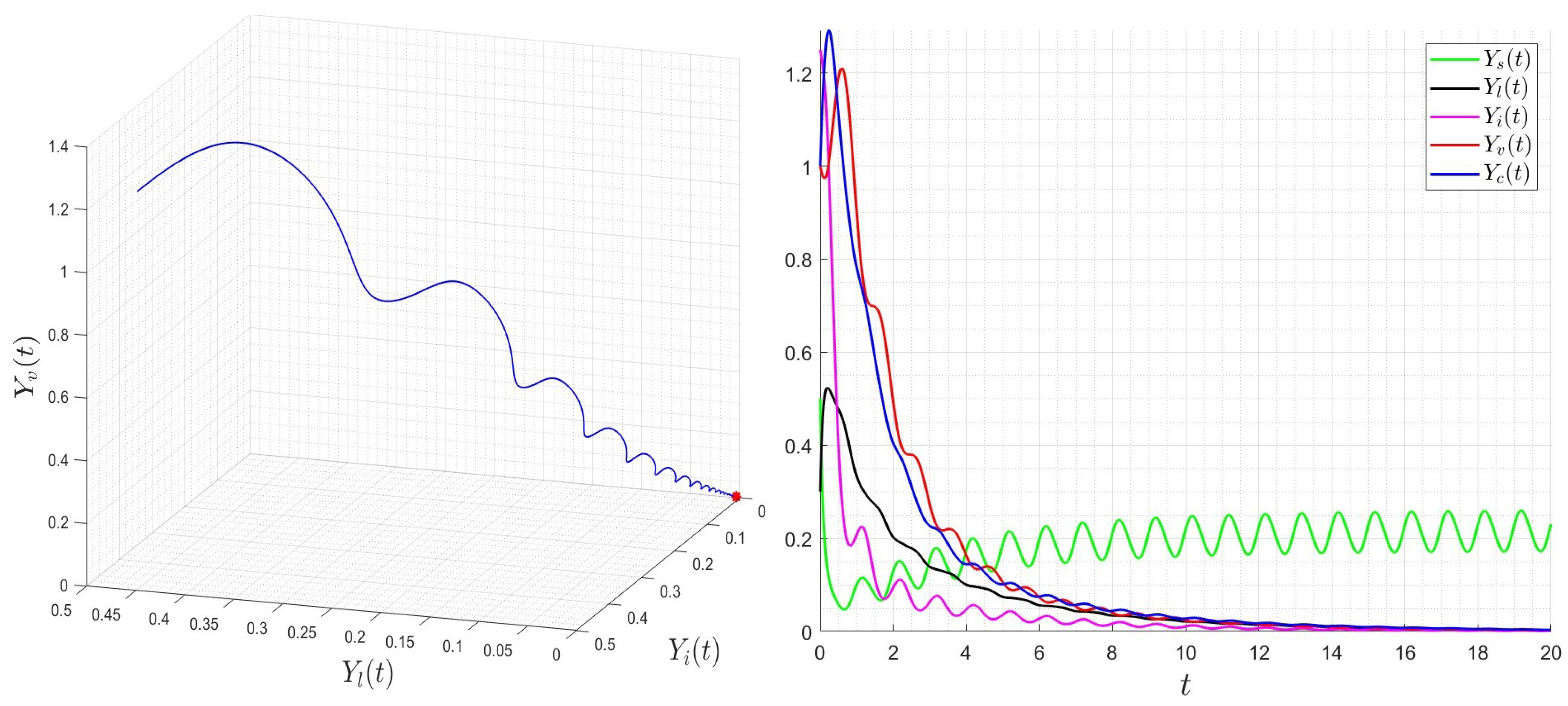
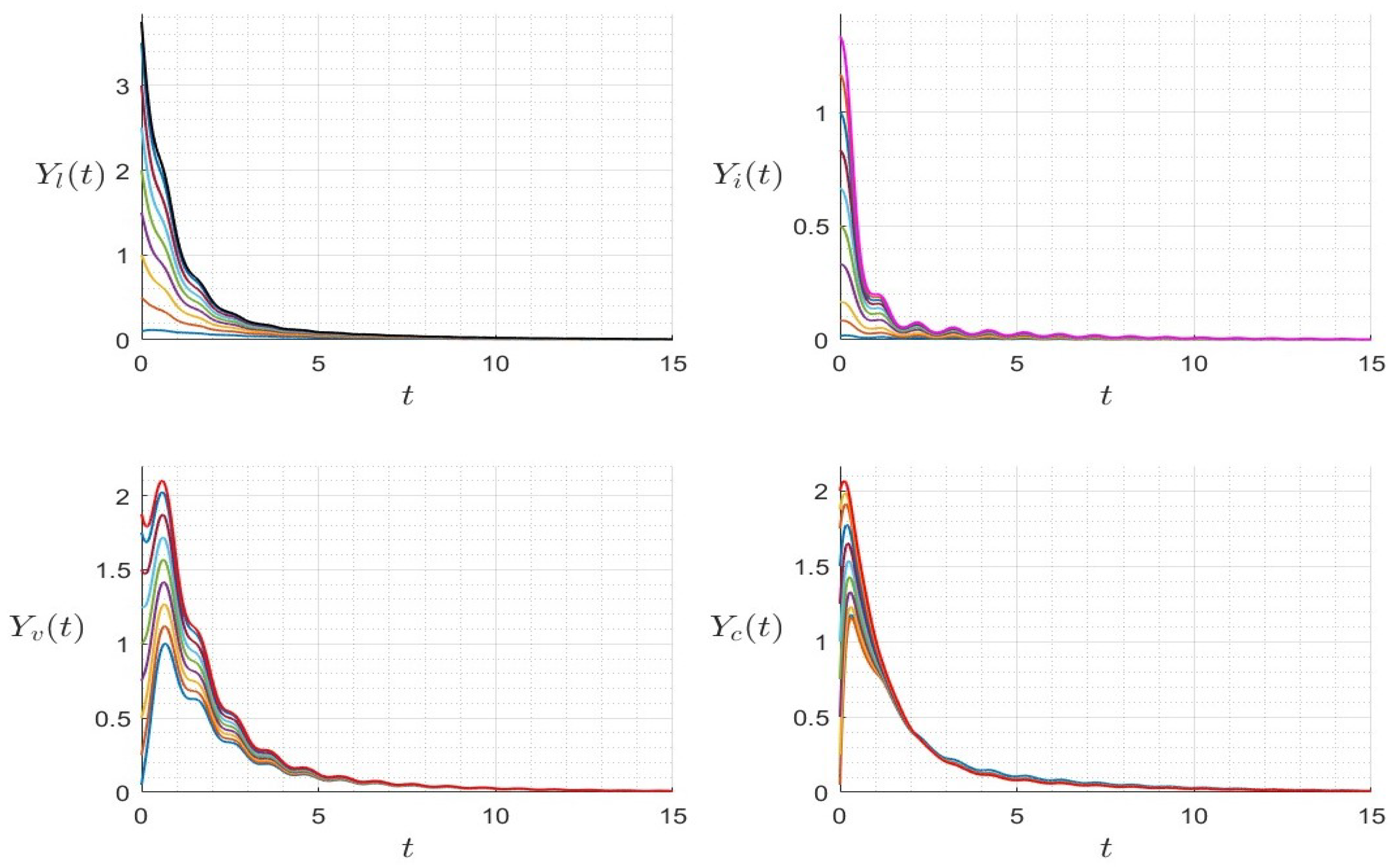
5. Numerical Examples

We illustrate the obtained theoretical results on the dynamics (1) by several numerical examples. The T-periodic functions that we used as model parameters are given hereafter.

$$\left\{\begin{array}{ccccccc}\hfill {\mathrm{\Lambda }}_{in}\left(t\right)& =\hfill & {\mathrm{\Lambda }}_{in0}(1+{\mathrm{\Lambda }}_{in1}cos\left(2\pi (t+\psi )\right)),\hfill & \hfill & \hfill d_s\left(t\right)& =\hfill & d_{s0}(1+d_{s1}cos\left(2\pi (t+\psi )\right)),\hfill \\ \hfill {\beta }_1\left(t\right)& =\hfill & {\beta }_{10}(1+{\beta }_{11}cos\left(2\pi (t+\psi )\right)),\hfill & \hfill & \hfill d_l\left(t\right)& =\hfill & d_{l0}(1+d_{l1}cos\left(2\pi (t+\psi )\right)),\hfill \\ \hfill {\beta }_2\left(t\right)& =\hfill & {\beta }_{20}(1+{\beta }_{21}cos\left(2\pi (t+\psi )\right)),\hfill & \hfill & \hfill d_i\left(t\right)& =\hfill & d_{i0}(1+d_{i1}cos\left(2\pi (t+\psi )\right)),\hfill \\ \hfill {\beta }_3\left(t\right)& =\hfill & {\beta }_{30}(1+{\beta }_{31}cos\left(2\pi (t+\psi )\right)),\hfill & \hfill & \hfill d_v\left(t\right)& =\hfill & d_{v0}(1+d_{v1}cos\left(2\pi (t+\psi )\right)),\hfill \\ \hfill \eta \left(t\right)& =\hfill & {\eta }_0(1+{\eta }_{1}cos\left(2\pi (t+\psi )\right)),\hfill & \hfill & \hfill d_c\left(t\right)& =\hfill & d_{c0}(1+d_{c1}cos\left(2\pi (t+\psi )\right)),\hfill \\ \hfill \gamma \left(t\right)& =\hfill & {\gamma }_0(1+{\gamma }_{1}cos\left(2\pi (t+\psi )\right)),\hfill & \hfill & \hfill \delta \left(t\right)& =\hfill & {\delta }_0(1+{\delta }_{1}cos\left(2\pi (t+\psi )\right)),\hfill \\ \hfill \epsilon \left(t\right)& =\hfill & {\epsilon }_0(1+{\epsilon }_{1}cos\left(2\pi (t+\psi )\right)),\hfill & \hfill & \hfill \lambda \left(t\right)& =\hfill & {\lambda }_0(1+{\lambda }_{1}cos\left(2\pi (t+\psi )\right)).\hfill \end{array}\right.$$

(22)

${\mathrm{\Lambda }}_{in1}$, $d_{s1}$, $d_{l1}$, $d_{i1}$, $d_{v1}$, $d_{c1}$, ${\beta }_{11}$, ${\beta }_{21}$, ${\beta }_{31}$, ${\eta }_1$, ${\gamma }_1$, ${\delta }_1$, ${\epsilon }_1$ and ${\lambda }_1$ are the amplitudes reflecting the influence of the variations on all of the parameters where $|{\mathrm{\Lambda }}_{in1}| <1$, $|d_{s1}| <1$, $|d_{l1}| <1$, $|d_{i1}| <1$, $|d_{v1}| <1$, $|d_{c1}| <1$, $|{\beta }_{11}| <1$, $|{\beta }_{21}| <1$, $|{\beta }_{31}| <1$, $|{\eta }_1| <1$, $|{\gamma }_1| <1$, $|{\delta }_1| <1$, $|{\epsilon }_1| <1$ and $|{\lambda }_1| <1$. The phase shift is given by $\psi$. All fixed constants used in the numerical examples are summarized in

Table 2. Constants used in the numerical examples.

${\mathbf{\Lambda }}_{\mathit{i}\mathit{n}0}$	${\mathit{d}}_{\mathit{s}0}$	${\mathit{d}}_{\mathit{l}0}$	${\mathit{d}}_{\mathit{i}0}$	${\mathit{d}}_{\mathit{v}0}$	${\mathit{d}}_{\mathit{c}0}$	${\mathit{\beta }}_{10}$	${\mathit{\beta }}_{20}$	${\mathit{\beta }}_{30}$	${\mathit{\eta }}_0$	${\mathit{\gamma }}_0$	${\mathit{\delta }}_0$	${\mathit{\epsilon }}_0$	${\mathit{\lambda }}_0$
10	$0.8$	$0.7$	2	$0.5$	1	$0.2$	$0.8$	4	2	$0.5$	1	$0.2$	$0.8$
${\mathbf{\Lambda }}_{\mathit{i}\mathit{n}\mathbf{1}}$	${\mathit{d}}_{\mathit{s}\mathbf{1}}$	${\mathit{d}}_{\mathit{l}\mathbf{1}}$	${\mathit{d}}_{\mathit{i}\mathbf{1}}$	${\mathit{d}}_{\mathit{v}\mathbf{1}}$	${\mathit{d}}_{\mathit{c}\mathbf{1}}$	${\mathit{\beta }}_{\mathbf{11}}$	${\mathit{\beta }}_{\mathbf{21}}$	${\mathit{\beta }}_{\mathbf{31}}$	${\mathit{\eta }}_{\mathbf{1}}$	${\mathit{\gamma }}_{\mathbf{1}}$	${\mathit{\delta }}_{\mathbf{1}}$	${\mathit{\epsilon }}_{\mathbf{1}}$	${\mathit{\lambda }}_{\mathbf{1}}$	$\mathit{\psi }$
10	$0.8$	$0.7$	2	$0.5$	1	$0.2$	$0.8$	4	2	$0.5$	1	$0.2$	$0.8$	4

.

Three environmental situations were considered. The first situation was dedicated to a totally fixed environment and all parameters are constants, and thus we obtain an autonomous system. We aim then to confirm the theoretical findings regarding the stability of the steady states ${\mathcal{E}}_0$ and ${\mathcal{E}}_{\ast }$. The second situation was dedicated to a variable contact, which means that only the contact rates ${\beta }_1\left(t\right)$, ${\beta }_2\left(t\right)$ and ${\beta }_3\left(t\right)$ are T-periodic, and the rest of the parameters are fixed. The third situation deals with a total variable environment such that all the parameters are T-periodic functions.

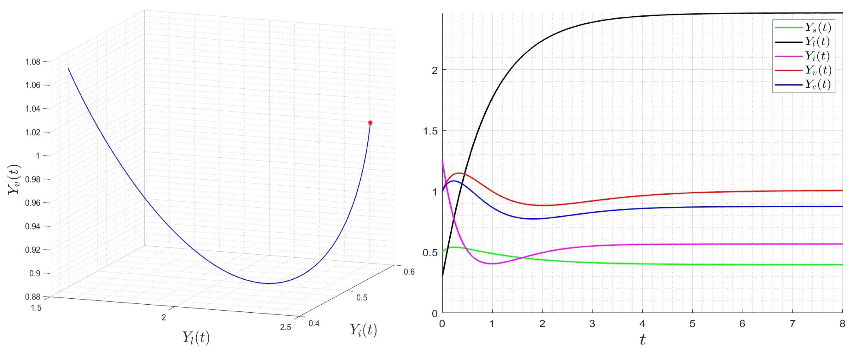
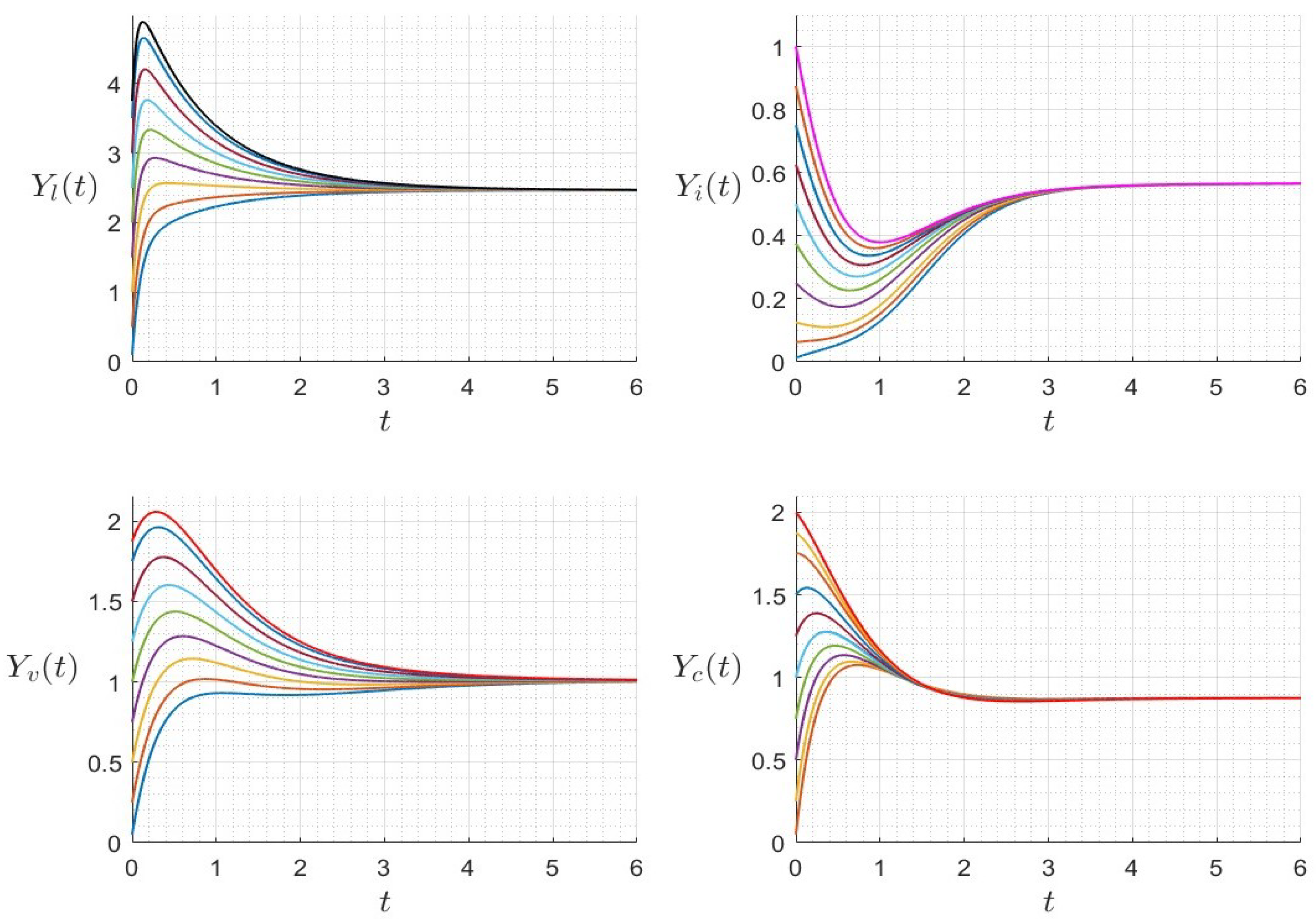
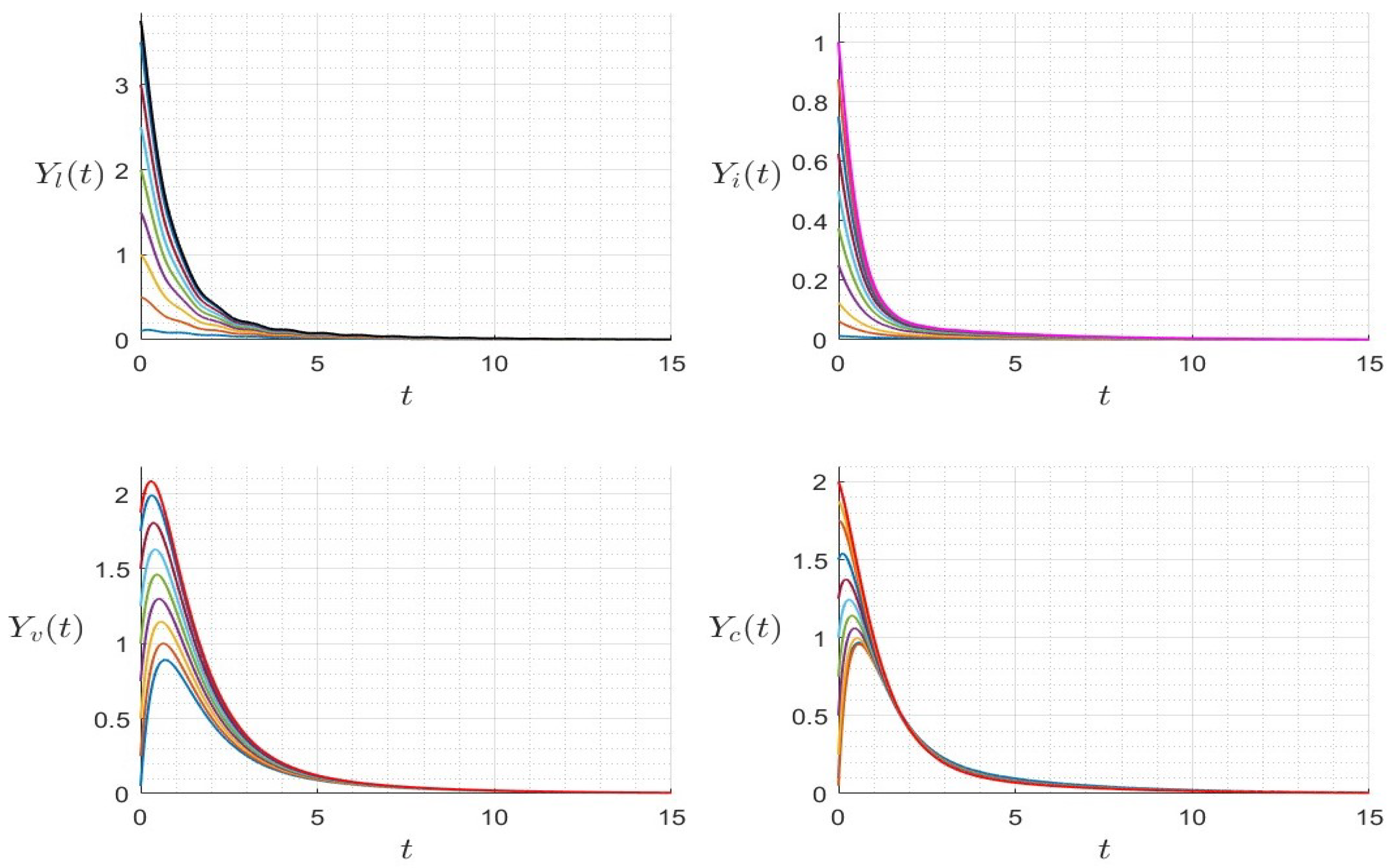
5.1. Totally Fixed Environment

We first consider the case of a totally fixed environment, and thus all the parameters of system (1) are constants as follows:

$$\left\{\begin{array}{c}\dot{Y_s}\left(t\right)=d_{s0}{\mathrm{\Lambda }}_{in0}-d_{s0}{Y}_s\left(t\right)-[{\beta }_{10}{Y}_v\left(t\right)+{\beta }_{20}{Y}_l\left(t\right)+{\beta }_{30}{Y}_i\left(t\right)]Y_s\left(t\right),\hfill \\ \dot{Y_l}\left(t\right)=[{\beta }_{10}{Y}_v\left(t\right)+{\beta }_{20}{Y}_l\left(t\right)+{\beta }_{30}{Y}_i\left(t\right)]Y_s\left(t\right)-({\eta }_0+d_{l0})Y_l\left(t\right),\hfill \\ \dot{Y_i}\left(t\right)={\eta }_0{Y}_l\left(t\right)-d_{i0}\left(t\right)Y_i\left(t\right)-{\gamma }_0{Y}_c\left(t\right)Y_i\left(t\right),\hfill \\ \dot{Y_v}\left(t\right)={\epsilon }_0{Y}_i\left(t\right)-d_{v0}{Y}_v\left(t\right),\hfill \\ \dot{Y_c}\left(t\right)={\lambda }_0{Y}_i\left(t\right)-d_{c0}{Y}_c\left(t\right)-{\delta }_0{Y}_c\left(t\right)Y_i\left(t\right),\hfill \end{array}\right.$$

(23)

with initial condition $(Y_s^0,Y_l^0,Y_i^0,Y_v^0,Y_c^0)=(10,10,6,8,10)\in {\mathbb{R}}_{+}^5$. We provide several numerical examples that confirm the stability of the steady states of (23). In Figure 1, we display the variables’ behavior when ${\mathcal{R}}_0<1$. The trajectory of the system (23) converges to the steady state ${\mathcal{E}}_0$, and this confirms the global stability of ${\mathcal{E}}_0$ when ${\mathcal{R}}_0\le 1$. In Figure 2, we display the behavior of all components of the solution for several initial conditions, confirming the global stability of ${\mathcal{E}}_0$ if ${\mathcal{R}}_0<1$. However, in Figure 3, we display the variables’ behavior when ${\mathcal{R}}_0>1$. The trajectory of the system (23) converges to the steady state ${\mathcal{E}}_{\ast }$, confirming the global stability of ${\mathcal{E}}_{\ast }$ when ${\mathcal{R}}_0>1$. In Figure 4, we display the behavior of all components of the solution for different initial conditions, confirming the global stability of ${\mathcal{E}}_{\ast }$ if ${\mathcal{R}}_0>1$.

5.2. Variable Contact Rates

Let us now perform numerical simulations on System (1) where only the variable forced T-periodic function $\beta$ depends on time, t. The other parameters are constant. Thus, the model is given by

$$\left\{\begin{array}{c}\dot{Y_s}\left(t\right)=d_{s0}{\mathrm{\Lambda }}_{in0}-d_{s0}{Y}_s\left(t\right)-[{\beta }_1\left(t\right)Y_v\left(t\right)+{\beta }_2\left(t\right)Y_l\left(t\right)+{\beta }_3\left(t\right)Y_i\left(t\right)]Y_s\left(t\right),\hfill \\ \dot{Y_l}\left(t\right)=[{\beta }_1\left(t\right)Y_v\left(t\right)+{\beta }_2\left(t\right)Y_l\left(t\right)+{\beta }_3\left(t\right)Y_i\left(t\right)]Y_s\left(t\right)-({\eta }_0+d_{l0})Y_l\left(t\right),\hfill \\ \dot{Y_i}\left(t\right)={\eta }_0{Y}_l\left(t\right)-d_{i0}\left(t\right)Y_i\left(t\right)-{\gamma }_0{Y}_c\left(t\right)Y_i\left(t\right),\hfill \\ \dot{Y_v}\left(t\right)={\epsilon }_0{Y}_i\left(t\right)-d_{v0}{Y}_v\left(t\right),\hfill \\ \dot{Y_c}\left(t\right)={\lambda }_0{Y}_i\left(t\right)-d_{c0}{Y}_c\left(t\right)-{\delta }_0{Y}_c\left(t\right)Y_i\left(t\right),\hfill \end{array}\right.$$

(24)

with positive initial condition $(Y_s^0,Y_l^0,Y_i^0,Y_v^0,Y_c^0)=(10,10,6,8,10)\in {\mathbb{R}}_{+}^5$. Note that ${\mathcal{R}}_0$ was calculated by using the time-averaged system as in [32,33]. Other definitions of ${\mathcal{R}}_0$ can be found in [34,35]. In Figure 5, we display the variables’ behavior when ${\mathcal{R}}_0<1$. The trajectory of the system (24) converges to the steady state ${\mathcal{E}}_0=\left({\mathrm{\Lambda }}_{in0},0,0,0,0,0\right)$, and this confirms the global stability of ${\mathcal{E}}_0$ when ${\mathcal{R}}_0\le 1$. In Figure 6, we display the behavior of all components of the solution for different initial conditions, confirming the global stability of ${\mathcal{E}}_0$ if ${\mathcal{R}}_0<1$. However, in Figure 7, we display the variables’ behavior when ${\mathcal{R}}_0>1$. The trajectory of the system (24) converges to the steady state ${\mathcal{E}}_{\ast }$, and this confirms the global stability of ${\mathcal{E}}_{\ast }$ when ${\mathcal{R}}_0>1$. In Figure 8, we display the behavior of all components of the solution for different initial conditions, confirming the global stability of ${\mathcal{E}}_{\ast }$ if ${\mathcal{R}}_0>1$.

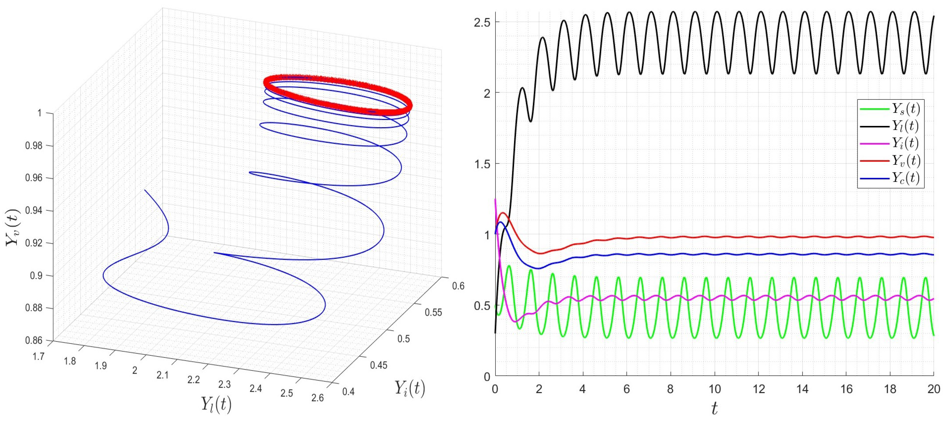
5.3. Totally Variable Environment

In this subsection, we consider the dynamics (1) such that all parameters are T-periodic functions as follows:

$$\left\{\begin{array}{c}\dot{Y_s}\left(t\right)=d_s\left(t\right){\mathrm{\Lambda }}_{in}\left(t\right)-d_s\left(t\right)Y_s\left(t\right)-[{\beta }_1\left(t\right)Y_v\left(t\right)+{\beta }_2\left(t\right)Y_l\left(t\right)+{\beta }_3\left(t\right)Y_i\left(t\right)]Y_s\left(t\right),\hfill \\ \dot{Y_l}\left(t\right)=[{\beta }_1\left(t\right)Y_v\left(t\right)+{\beta }_2\left(t\right)Y_l\left(t\right)+{\beta }_3\left(t\right)Y_i\left(t\right)]Y_s\left(t\right)-(\eta \left(t\right)+d_l\left(t\right))Y_l\left(t\right),\hfill \\ \dot{Y_i}\left(t\right)=\eta \left(t\right)Y_l\left(t\right)-d_i\left(t\right)Y_i\left(t\right)-\gamma \left(t\right)Y_c\left(t\right)Y_i\left(t\right),\hfill \\ \dot{Y_v}\left(t\right)=\epsilon \left(t\right)Y_i\left(t\right)-d_v\left(t\right)Y_v\left(t\right),\hfill \\ \dot{Y_c}\left(t\right)=\lambda \left(t\right)Y_i\left(t\right)-d_c\left(t\right)Y_c\left(t\right)-\delta \left(t\right)Y_c\left(t\right)Y_i\left(t\right),\hfill \end{array}\right.$$

(25)

with positive initial condition $(Y_s^0,Y_l^0,Y_i^0,Y_v^0,Y_c^0)=(10,10,6,8,10)\in {\mathbb{R}}_{+}^5$. Similarly to the case of system (24), ${\mathcal{R}}_0$ was calculated using a time-averaged system as in [32,33]. We presented several numerical examples confirming the asymptotic stability of dynamics (25). In Figure 9, we display the variables’ behavior when ${\mathcal{R}}_0<1$. The trajectory of the system (25) converges to the free-virus periodic state ${\mathcal{E}}_0\left(t\right)=(Y_s^{\ast }\left(t\right),0,0,0,0,0)$, confirming the global stability of ${\mathcal{E}}_0\left(t\right)$ when ${\mathcal{R}}_0\le 1$. In Figure 10, we display the behavior of all components of the solution with several initial conditions, confirming the global stability of ${\mathcal{E}}_0\left(t\right)$ if ${\mathcal{R}}_0<1$. However, in Figure 11, we display the variables’ behavior when ${\mathcal{R}}_0>1$. The trajectory of the system (25) converges asymptotically to a periodic solution reflecting the virus’ persistence when ${\mathcal{R}}_0>1$. In Figure 12, we display the behavior of all components of the solution with several initial conditions. The solution converges to a periodic trajectory with persistence of the virus. when ${\mathcal{R}}_0>1$.

6. Conclusions

In this study, we extended the HIV dynamics model already studied in [12] by considering a variable environment. The model explored three routes of infection including the HIV-to-cell contact, latently infected cell-to-cell contact, and actively infected cell-to-cell contact. In the first stage, we analyzed the case of a fixed environment, such that all parameters are fixed positive constants. In the second stage, we considered the case of a variable environment, where we defined the basic reproduction number ${\mathcal{R}}_0$. We proved the global stability of the virus-free periodic trajectory, ${\mathcal{E}}_0\left(t\right)$ if ${\mathcal{R}}_0<1$. However, we proved that the virus will persist if ${\mathcal{R}}_0>1$ and the solution converges to a periodic trajectory. We confirmed the obtained results by several numerical examples, including the fixed environment, the variable contact rates, and the fully variable environment. The trajectories converged to one of the steady states of (2), confirming Theorems 2 and 3, in the case of the fixed environment. Since at least the contact rates are periodic, the solution of (1) will be periodic and converges to a limit cycle confirming Theorems 5 and 6.

References

1. Perelson, A.S.; Neumann, A.U.; Markowitz, M.; Leonard, J.M.; Ho, D.D. HIV-1 dynamics in vivo: Virion clearance rate, infected cell life-span, and viral generation time. Science 1996, 271, 1582–1586. [Google Scholar] [CrossRef] [PubMed]
2. Nowak, M.A.; Bonhoeffer, S.; Shaw, G.M.; May, R.M. Anti-viral Drug Treatment: Dynamics of Resistance in Free Virus and Infected Cell Populations. J. Theor. Biol. 1997, 184, 203–217. [Google Scholar] [CrossRef] [PubMed]
3. Perelson, A.S.; Essunger, P.; Cao, Y.; Vesanen, M.; Hurley, A.; Saksela, K.; Markowitz, M. Decay characteristics of HIV-1-infected compartments during combination therapy. Nature 1997, 387, 188–191. [Google Scholar] [CrossRef] [PubMed]
4. De Boer, R.; Perelson, A. Target Cell Limited and Immune Control Models of HIV Infection: A Comparison. J. Theor. Biol. 1998, 190, 201–214. [Google Scholar] [CrossRef] [PubMed]
5. Wodarz, D.; Lloyd, A.L.; Jansen, V.A.; Nowak, M.A. Dynamics of Macrophage and T Cell Infection by HIV. J. Theor. Biol. 1999, 196, 101–113. [Google Scholar] [CrossRef] [PubMed]
6. Bajaria, S.H.; Webb, G.; Kirschner, D.E. Predicting differential responses to structured treatment interruptions during HAART. Bull. Math. Biol. 2004, 66, 1093–1118. [Google Scholar] [CrossRef] [PubMed]
7. Elaiw, A.; AlShamrani, N. Stability of a general CTL-mediated immunity HIV infection model with silent infected cell-to-cell spread. Adv. Differ. Equ. 2020, 2020, 335. [Google Scholar] [CrossRef]
8. AlShamrani, N. Stability of a general adaptive immunity HIV infection model with silent infected cell-to-cell spread. Chaos Solitons Fractals 2021, 150, 110422. [Google Scholar] [CrossRef]
9. Alsahafi, S.; Woodcock, S. Exploring HIV Dynamics and an Optimal Control Strategy. Mathematics 2022, 10, 749. [Google Scholar] [CrossRef]
10. Stengel, R.F. Mutation and control of the human immunodeficiency virus. Math. Biosci. 2008, 213, 93–102. [Google Scholar] [CrossRef]
11. Starkov, K.E.; Kanatnikov, A.N. Eradication Conditions of Infected Cell Populations in the 7-Order HIV Model with Viral Mutations and Related Results. Mathematics 2021, 9, 1862. [Google Scholar] [CrossRef]
12. AlShamrani, N.H.; Halawani, R.H.; Shammakh, W.; Elaiw, A.M. Global Properties of HIV-1 Dynamics Models with CTL Immune Impairment and Latent Cell-to-Cell Spread. Mathematics 2023, 11, 3743. [Google Scholar] [CrossRef]
13. Xiao, D. Dynamics and bifurcations on a class of population model with seasonal constant-yield harvesting. Discret. Contin. Dyn. Syst. -B 2016, 21, 699–719. [Google Scholar] [CrossRef]
14. Ibrahim, M.A.; Dénes, A. Stability and Threshold Dynamics in a Seasonal Mathematical Model for Measles Outbreaks with Double-Dose Vaccination. Mathematics 2023, 11, 1791. [Google Scholar] [CrossRef]
15. Bacaër, N.; Guernaoui, S. The epidemic threshold of vector-borne diseases with seasonality. J. Math. Biol. 2006, 53, 421–436. [Google Scholar] [CrossRef]
16. Bacaër, N. Approximation of the basic reproduction number R0 for vector-borne diseases with a periodic vector population. Bull. Math. Biol. 2007, 69, 1067–1091. [Google Scholar] [CrossRef]
17. Ibrahim, M.A.; Dénes, A. A mathematical model for Lassa fever transmission dynamics in a seasonal environment with a view to the 2017–20 epidemic in Nigeria. Nonlinear Anal. Real World Appl. 2021, 60, 103310. [Google Scholar] [CrossRef]
18. El Hajji, M.; Alshaikh, D.M.; Almuallem, N.A. Periodic behaviour of an epidemic in a seasonal environment with vaccination. Mathematics 2023, 11, 2350. [Google Scholar] [CrossRef]
19. El Hajji, M.; Alnjrani, R.M. Periodic Trajectories for HIV Dynamics in a Seasonal Environment With a General Incidence Rate. Int. J. Anal. Appl. 2023, 21, 96. [Google Scholar] [CrossRef]
20. El Hajji, M. Periodic solutions for chikungunya virus dynamics in a seasonal environment with a general incidence rate. AIMS Math. 2023, 8, 24888–24913. [Google Scholar] [CrossRef]
21. Diekmann, O.; Heesterbeek, J. On the definition and the computation of the basic reproduction ratio R0 in models for infectious diseases in heterogeneous populations. J. Math. Biol. 1990, 28, 365–382. [Google Scholar] [CrossRef]
22. Den Driessche, P.V.; Watmough, J. Reproduction Numbers and Sub-Threshold Endemic Equilibria for Compartmental Models of Disease Transmission. Math. Biosci. 2002, 180, 29–48. [Google Scholar] [CrossRef]
23. Hurwitz, A. Ueber die Bedingungen, unter welchen eine Gleichung nur Wurzeln mit negativen reellen Theilen besitzt. (English translation “On the conditions under which an equation has only roots with negative real parts” by H. G. Bergmann in Selected Papers on Mathematical Trends in Control Theory R. Bellman and R. Kalaba Eds. New York: Dover, 1964; pp. 70–82). Math. Ann. 1895, 46, 273–284. [Google Scholar]
24. Routh, E.J. A Treatise on the Stability of a Given State of Motion: Particularly Steady Motion; Macmillan: New York, NY, USA, 1877. [Google Scholar]
25. El Hajji, M. Mathematical modeling for anaerobic digestion under the influence of leachate recirculation. AIMS Math. 2023, 8, 30287–30312. [Google Scholar] [CrossRef]
26. LaSalle, J. The Stability of Dynamical Systems; SIAM: Philadelphia, PA, USA, 1976. [Google Scholar]
27. Alshehri, A.; El Hajji, M. Mathematical study for Zika virus transmission with general incidence rate. AIMS Math. 2022, 7, 7117–7142. [Google Scholar] [CrossRef]
28. Frobenius, G. Uber Matrizen aus Nicht Negativen Elementen; Sitzungsberichte Preussische Akademie der Wissenschaft: Berlin, Germany, 1912; pp. 456–477. [Google Scholar]
29. Zhang, F.; Zhao, X. A periodic epidemic model in a patchy environment. J. Math. Anal. Appl. 2007, 325, 496–516. [Google Scholar] [CrossRef]
30. Wang, W.; Zhao, X. Threshold dynamics for compartmental epidemic models in periodic environments. Dynam. Differ. Equ. 2008, 20, 699–717. [Google Scholar] [CrossRef]
31. Zhao, X. Dynamical Systems in Population Biology; CMS Books in Mathematics (CMSBM); Springer: New York, NY, USA, 2003; Volume 16. [Google Scholar]
32. Ma, J.; Ma, Z. Epidemic threshold conditions for seasonally forced SEIR models. Math. Biosci. Eng. 2006, 3, 161–172. [Google Scholar] [CrossRef]
33. Zhang, T.; Teng, Z. On a nonautonomous SEIRS model in epidemiology. Bull. Math. Biol. 2007, 69, 2537–2559. [Google Scholar] [CrossRef]
34. Guerrero-Flores, S.; Osuna, O.; de Leon, C.V. Periodic solutions for seasonal SIQRS models with nonlinear infection terms. Electron. J. Differ. Equations 2019, 2019, 1–13. [Google Scholar]
35. Nakata, Y.; Kuniya, T. Global dynamics of a class of SEIRS epidemic models in a periodic environment. J. Math. Anal. Appl. 2010, 363, 230–237. [Google Scholar] [CrossRef]
Figure 1. Behavior of dynamics (23) for Λ i n 0 = 0.2 then R 0 0.6364 < 1 . The red star describe the limit (final state) of the variable ( Y l , Y i , Y v ) .
Mathematics 12 00123 g001
Figure 2. Behavior of dynamics (23) for several initial conditions where Λ i n 0 = 0.2 ( R 0 0.6364 < 1 ). The different graphs (colors) reflect different initial conditions.
Mathematics 12 00123 g002
Figure 3. Behavior of dynamics (23) for Λ i n 0 = 2 then R 0 6.3642 > 1 . The red star describe the limit (final state) of the variable ( Y l , Y i , Y v ) .
Mathematics 12 00123 g003
Figure 4. Behavior of dynamics (23) for several initial conditions where Λ i n 0 = 2 ( R 0 6.3642 > 1 ). The different graphs (colors) reflect different initial conditions.
Mathematics 12 00123 g004
Figure 5. Behavior of dynamics (24) for Λ i n 0 = 0.2 then R 0 0.6364 < 1 . The red star describe the limit (final state) of the variable ( Y l , Y i , Y v ) .
Mathematics 12 00123 g005
Figure 6. Behavior of dynamics (24) for several initial conditions where Λ i n 0 = 0.2 ( R 0 0.6364 < 1 ). The different graphs (colors) reflect different initial conditions.
Mathematics 12 00123 g006
Figure 7. Behavior of dynamics (24) for Λ i n 0 = 2 then R 0 6.3642 > 1 . The red curve describe the limit-cycle of the variable ( Y l , Y i , Y v ) .
Mathematics 12 00123 g007
Figure 8. Behavior of dynamics (24) for several initial conditions where Λ i n 0 = 2 ( R 0 6.3642 > 1 ). The different graphs (colors) reflect different initial conditions.
Mathematics 12 00123 g008
Figure 9. Behavior of dynamics (25) for Λ i n 0 = 0.2 then R 0 0.6364 < 1 . The red star describe the limit (final state) of the variable ( Y l , Y i , Y v ) .
Mathematics 12 00123 g009
Figure 10. Behavior of dynamics (25) for several initial conditions where Λ i n 0 = 0.2 ( R 0 0.6364 < 1 ). The different graphs (colors) reflect different initial conditions.
Mathematics 12 00123 g010
Figure 11. Behavior of dynamics (25) for Λ i n 0 = 2 ( R 0 6.3642 > 1 ). The red curve describe the limit-cycle of the variable ( Y l , Y i , Y v ) .
Mathematics 12 00123 g011
Figure 12. Behavior of dynamics (25) for several initial conditions where Λ i n 0 = 2 ( R 0 6.3642 > 1 ). The different graphs (colors) reflect different initial conditions.
Mathematics 12 00123 g012