1. Introduction
Our skeleton, a mechanical structure consisting of 206 pieces, provides safe shelter for vital organs, transforms the force created by muscle contraction into locomotion, and is a suitable reservoir for ions (notably calcium) involved in many physiological processes [
1]. The skeleton is a dynamic organ that can alter the mass and architecture of its individual elements, the bones, to accommodate a range of mechanical environments. Thus, the bones affected by a local increase in load respond by locally increasing the resistance of the bone tissue, and, conversely, regionally decreasing load results in reduced bone mass [
2]. Clearly, so complex a structure needs careful and timely monitoring and repair to ensure that its compliance is permanently ensured. The process whereby such goals are achieved is termed bone remodeling (BR). More precisely, BR denotes the continual destruction (resorption) and rebuilding process that takes place in the bones of a mature skeleton throughout the lifetime of the organism. Bone remodeling becomes routine after the skeleton reaches its adult structure, which is achieved by means of a previous stage known as bone modeling, which is not considered in this work. For further details on key aspects of bone remodeling, we refer the reader to ref. [
3] where a thorough, updated outline of the meaning and relevance on that problem in Medicine and Biology can be found. Classical presentations, in line with the views of the pioneers in this field, can be found in refs. [
4,
5,
6,
7]. Finally, an interdisciplinary approach where attention is paid to the mathematical modeling of bone remodeling is provided in refs. [
8,
9].
It was initially thought that bone remodeling was a homeostatic response to repair microscopic bone damage resulting from microfractures. This was the starting viewpoint of a pioneer in the field, Harold Frost, who, during the 1960s, introduced the concept of the Bone Multicellular Unit, BMU [
4,
5,
10,
11], to explain how BR is carried out in cortical bone. BMUs are transient functional groups of cells operating in a concerted and coordinated fashion that are composed of osteoclasts, which first destroy the old bone matrix, and osteoblasts, which subsequently form the new matrix. Once the cavity left behind by osteoclasts is filled, some osteoblasts become trapped there to eventually differentiate into osteocytes, the most common cell type in bones. Then, the matrix surrounding them (which remains pervaded by osteocyte-linking canaliculi) becomes mineralized, thus marking the end of the remodeling event; see, for instance, [
8,
9]. Concerning the time and space scales at which BMUs operate, a lifespan of 6–9 months for a BMU has been reported, during which a bone volume of 0.025 mm
is replaced [
6,
12].
In the aforementioned case, BR provides a repair mechanism that restores the integrity and mechanical resistance of a bone challenged by microfractures. However, it has long since been suspected that this process might be designed to address other needs as well. For instance, it has been hypothesized that there may be BMU-mediated nontargeted remodeling to maintain the age of the bone tissue below some upper limit, even when no repair action is immediately needed at those places [
7,
13]. For instance, and as reviewed in [
14], BMU-mediated remodeling is thought to play a significant role in calcium homeostasis, which may lead to increased bone resorption to provide adequate levels of serum calcium. Moreover, BR is the only mechanism known by which senescent, dying, or dead osteocytes may be replaced [
14]. In general, a thorough, periodic bone screening seems necessary to avoid systemic collapse being induced by the simultaneous presence of many BR events, as well as to preclude that the coalescence of microcracks may result in the origin of large (and dangerous) fractures, a well-known fact in structural mechanics [
15,
16,
17].
As a consequence of the evidence recalled in the previous remarks, it is nowadays customary to consider that there are two basic types of bone remodeling:
targeted, which is induced by local injuries resulting in microfractures, and
nontargeted. This last term includes remodeling induced by other reasons, some of which have been mentioned above. In fact, nontargeted bone remodeling is often supposed to be a stochastic process [
3,
7]. Importantly, it is commonly accepted that bone remodeling, whether targeted or nontargeted, is responsible for the full renewal of the skeleton periodically in time. In particular, the time interval between successive remodeling events at the same bone location has been proposed to lie between 2 and 5 years, and a turnover of the whole skeleton of 10% per year has been suggested [
6,
12]. This last figure has led to the widely accepted assumption that our whole skeleton is fully renewed every 10 years, approximately [
3,
14]. Furthermore, it is estimated that in healthy human adults, 3–4 million BMUs are initiated per year, and about 1 million are at work at any given moment [
12].
The goal of this paper is to explore a possible mechanism to explain the periodic screening of the whole skeleton as well as the triggering of nontargeted bone remodeling which accounts for its periodical full renewal. More precisely, we propose here a proof-of-concept argument consisting of a simple class of computational algorithms, based on well-known biological rules, that have the following properties:
- (i)
Thorough screening capability of the surface explored,
- (ii)
Algorithmic operating rules that are based on individual decisions taken by a small number of agents, which represent the basic cell types involved: osteocytes, osteoclasts, osteoblasts and their precursors.
In fact, instead of focusing on the interactions between the many molecular agents possibly involved (reviewed in [
3]; see also [
8]), we intend to provide a picture, as simple as possible, of how a self-running, efficient decision algorithm could be identified that accounts for the key aspects of bone remodeling that were recalled above. This article can be seen as a further step in the program developed in previous research of our group [
8,
9]. More precisely, in [
8], a mathematical model was proposed to represent the dynamics of the BMUs, which first degrade a concrete area of the bony tissue and then rebuild it once bone remodeling was started there. The question of how BMUs are related to bone scanning mechanisms was left open there. On the other hand, in [
9], we described a screening mechanism that can periodically scan any single, flat bone piece, but no interface between the screening and remodeling process addressed was provided. In this work, we propose an integrated mechanism accounting for the interaction between screening and remodeling, thus providing a missing link between the approaches developed in these previous studies.
More precisely, the plan of this article is as follows. The class of biologically inspired algorithms considered here is explained in
Section 2. In summary, the logic of these algorithms is inspired by the mode of action of sclerostin, a small glycoprotein secreted by osteocytes that inhibits bone formation by preventing osteoblast differentiation. Based on the short-range (paracrine) effect of sclerostin [
18], we assume that changes in the production of this protein by any osteocyte are determined by the levels of sclerostin expression in its immediate neighbor osteocytes, a behavior that can be naturally modeled within the framework of cellular automata. We show that, out of the many algorithms that can be constructed according to this principle, only a part meets the criteria required for bone homeostasis and is compatible with (i) and (ii) above, such as, for instance,
- (i)
Exhaustive and periodic scanning of any given bone,
- (ii)
A limit on the number of remodeling events sustained by any bone piece at a given time,
- (iii)
Robustness with respect to minor perturbations in the algorithmic decision rules.
Moreover, the algorithms proposed can be linked, in a modular manner, with additional decision rules accounting, for instance, for biochemical signaling networks and their possible feedback loops. In this way, increasingly complex technical ingredients might be added to deal with intricate mechanisms corresponding to bone remodeling under different situations, arising from different external inputs on single bone pieces. Some examples are discussed in
Section 3, where the response of our algorithms to microfractures is also analyzed. Finally, a discussion of the results obtained is contained in
Section 4. In
Appendix A we provide a description of the computational algorithms considered and a basic pseudo-code that is also included in Listing A1.
2. Materials and Methods
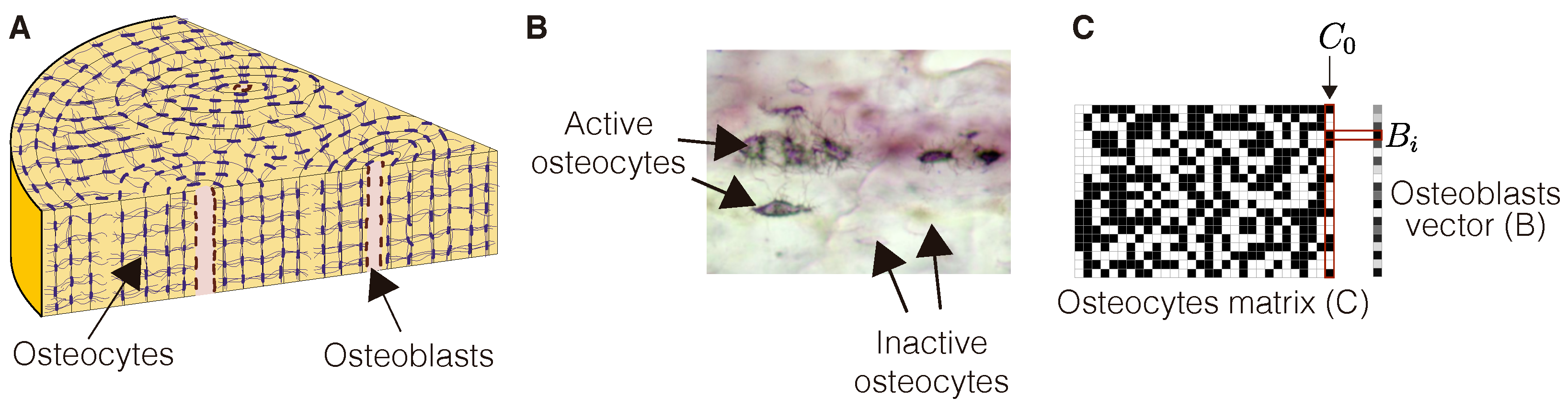
Bone remodeling is known to start when osteoblast precursors lining the bone boundaries are activated, a fact that crucially depends on the production of sclerostin by osteocytes, the more common type of bone resident cells. Osteocytes are distributed within the bone matrix, forming a network intercommunicated by canaliculi (see
Figure 1). Sclerostin is known to inhibit the activation of osteoblasts [
18]. We assume that this action is mediated by an inhibitory molecule acting on osteoblasts. In order to better explain the proposed mechanisms, we consider here a simple scenario, roughly equivalent to a planar section of the bone (see
Figure 1). In particular, osteocytes are assumed to occupy a two-dimensional matrix,
, of
cells. Our choice of cellular automata relies on two key features of osteocytes. First, they exhibit a regular spatial arrangement in the bone, as seen in
Figure 1. Second, these cells can be in one of two discrete states regarding sclerostin production (
Figure 1C). We refer to these states as active (and label as 1) when they produce sclerostin, and inactive (labeled as 0) otherwise. We assume that changes in the concentration of sclerostin in any osteocyte depend on the amount of such protein in its immediate neighbors, as is detailed further. The spatial arrangement of active and inactive osteocytes, as shown in
Figure 1, provides a natural setting to define a cellular automata algorithm.
For simplicity, we suppose that each osteoblast (which occupies a box in the column B in
Figure 1C) is under the influence of a single, adjacent osteocyte (the closest one in the adjacent row). An increase in the production of sclerostin in any such osteocyte results in an increase in the amount of inhibitor in the associated osteoblast. If the osteocyte is inactive (not producing sclerostin), the inhibitor in that osteoblast is assumed to decrease linearly in time. When the amount of such inhibitor falls below a critical level, the osteoblast is turned on, osteoclasts precursors are called in, and a remodeling event begins [
8]. When this occurs, the whole osteocyte row associated to that osteoblast becomes inactive. The question addressed here is whether such algorithms ensure that any single piece of the bone region under consideration is checked over and over again.
In cellular automata algorithms, the state of each cell at any time depends on the state of its neighbors. The dynamics of the model are dictated by transition rules that determine the state of each cell at iteration as a function of the state of its neighbors at iteration t. In this article, we consider a particular, large enough class of cellular automata which suffices to illustrate the decision rules we want to propose as possible algorithms underlying bone remodeling.
We assume that each osteocyte is under the influence of its eight nearest neighbors only. A transition rule can be described as an array of zeros and ones of length 18. The first (respectively, last) nine positions indicate the transition of inactive (respectively, active) osteocytes that have zero to eight active neighbors. A particular illustration of this type of rules is provided in
Figure 2.
In this work, we consider a class of transition rules of which the previous example is a particular case. Specifically, we define the following classes of functions:
We let
i denote the state of an osteocyte, where at any simulation step we write
when it is inactive and
when it is active. Transition rule
prescribes the state of such osteocyte at the next simulation step if it has
n active neighbors. Then, transition rule
T consists in a choice of two functions,
, belonging to set
so that
We notice that in our previous example, we have if and otherwise, and if or and otherwise.
Our choice is motivated by the assumption that these parsimonious transition rules would be easy to implement in real osteocytes. In fact, these rules only require for osteocytes to determine whether the number of their active neighbors is above or below a certain threshold. To obtain the dynamics encoded in any such algorithm, for each transition rule satisfying (
1), we perform 1000 iterations of the model starting from an initial condition in which all osteocytes are inactive.
The behavior of osteoblasts is modeled as follows. First, we consider array
of osteoblasts and assume that they are in contact with a fixed column of osteocytes. We label this column as
. This configuration is equivalent to assuming that each osteoblast
is controlled by a single osteocyte (
) (see
Figure 1). We further assume that the activity of each osteoblast is inhibited by intracellular molecule
, whose levels in each cell are determined by the production of sclerostin in the adjoint osteocyte according to the following equation:
where
is the amount of inhibitor in osteoblast
i,
is the state of osteocyte
at iteration
t, so that
if
is active at time
t, and
otherwise, and
and
are positive constants. This equation implies that the amount of inhibitor increases when the osteocyte is active and decreases otherwise. We assume that osteoblasts trigger a remodeling event when their level of inhibitor reaches a threshold lower value that for simplicity we set equal to zero. The remodeling event of osteoblast
entails the death of all osteocytes in row
, which is modeled by setting the state of these cells to zero, i.e.,
In the next iteration, their state is updated according to the current transition rule. The state of all osteocytes and osteoblasts is updated synchronously. For convenience of the reader, a pseudocode of an algorithm of this kind is provided in
Appendix A.
Clearly, a huge number of algorithms could be formulated along the rules sketched above. However, bone homeostasis sets tight limits to the possible choices of transition rules. For instance, too many remodeling events taking place at the same time in a single bone should be avoided, since the integrity of that bone might otherwise be compromised. Bearing this remark in mind, we discard transition rules that permit simultaneous activation of osteoblasts above some threshold percentage, which are set at 15% for definiteness. On the other hand, actual algorithms should be robust. More precisely, we consider the effect of small changes in the production of sclerostin in osteocytes, which result in the replacement of a transition rule by another one, and discuss the impact of such changes on the remodeling process. These issues are examined in detail in
Section 3 below.
3. Results
We now present the results of numerical simulations comparing the performance of various algorithms corresponding to different choices of transition rules. Such rules differ from each other in their requirements on the number of active neighbors that determine the change in state (active, inactive) of any osteocyte. The corresponding conditions can be encoded in a sequence of 18 digits. For instance, the algorithm described in
Figure 2 corresponds to the following sequence:
For the ease of notation, it is convenient to replace sequences as (
4) by their binary representation. This is achieved by considering (
4) as a sum of powers of two in descending order left to right, beginning with
and with coefficients one, zero as shown in that sequence. In particular, for (
4), the corresponding number is 153441. We use this decimal representation to label the algorithms to be subsequently discussed.
Figure 3 shows the numerical simulations of the model for different choices of transition rules. Such rules differ from each other in the conditions that determine the change in state of osteocytes as a function of the number of active osteocyte neighbors. The emerging dynamics are quite heterogeneous, and many of them give rise to non-suitable remodeling strategies. For instance, in rule 131,072 in
Figure 3A, osteocytes switch from inactive to active states and back sequentially in time (inactive at
, active at
, inactive at
, …). In view of Equation (
3), it takes longer for osteoblasts to be activated if the initial amount of their inhibitor is positive. However, at suitable times (
, …; see details in
Appendix A) in our simulation, all of them are turned on to become inactive again in intermediate times. Such type of mechanism results in the simultaneous remodeling of the whole bone, which compromises its integrity and therefore should be avoided. We remark in passing that, since 131,072 = 2
, such rule corresponds to digit sequence 10000000000000000, which prescribes that osteocytes are activated only when all their neighbors are inactive.
A different behavior is represented by rule 16,895 in
Figure 3A. In this case, some osteoblasts trigger periodic remodeling events, but most of them are never activated. This pattern of osteoblast activation does not simulate the required dynamics of bone remodeling, since large regions of the bone are never scanned. Other transition rules (7807, 7675 or 57,847 in
Figure 3A, for instance) also give rise to non-realistic mechanisms of bone remodeling.
Some transition rules (
Figure 3B) succeed in producing temporal and spatial patterns of bone scanning according to admissible behaviors. Such rules differ in the particular details of the pattern of the bone scan they produce. In the case of rule 25,057, for instance, remodeling events are frequent, and many osteoblasts are simultaneously active. In contrast, under rule 163,832, remodeling events are rare, and only a few cells are activated at the same time. This can be seen in more detail in
Figure 3C,D. Considering that biological sound algorithms should trigger bone remodeling events in every bone region, we assume that all osteoblasts must activate at least once for a transition rule to be admissible (
Figure 3D).
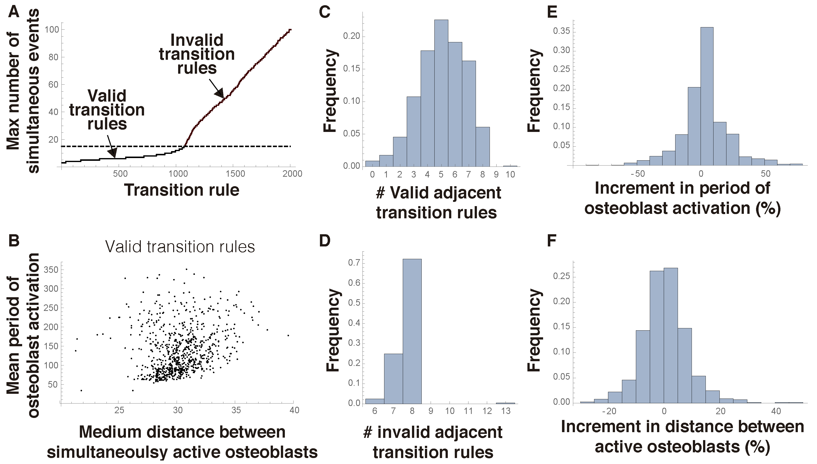
We next address the issue of the robustness of admissible transition rules. To that end, we first consider a set of 2000 transition rules randomly chosen. Then, for each of them, we consider all its adjacent rules, defined as those that differ in 1 of the 18 digits in its representing sequence. Finally, we analyze the validity of the adjacent transition rules thus generated. In this regard, a condition that homeostatic algorithms should satisfy is that the fraction of osteoblasts that are simultaneously active must be below a critical threshold (for definiteness, we selected here a 15% percentage as that value).
Figure 4A shows that many rules are invalid under this criterium. We next analyze the set of valid rules. To that end, we begin by considering two variables: the distance between osteoblasts that are simultaneously active and the period of osteoblast activation. A cluster of close cells that activate at the same time may hint at a local fragility of the bone, meaning that this rule is biologically deficient. As for the period between individual osteoblast activation times, it is a measure of the dynamism of the mechanism of bone remodeling. A shorter period implies a faster scan of the bone. A conclusion that can be drawn from
Figure 4B is that the logic of spatial computation suggested in this work gives rise to a wide range of realistic mechanisms of bone remodeling. We notice that bones in different body parts of a vertebrate or in the same bone in different species may be subject to different remodeling rates in response to different mechanical environments. This can be modulated by varying the responsiveness of osteocytes to sclerostin production by their neighbors.
Figure 4C,D show the probability of obtaining a valid or invalid rule by slightly changing a valid rule. The mode of the distribution of valid neighboring rules is five, while that of invalid rules is eight. The latter means that an admissible algorithm may perform poorly when comparatively minor modifications in its transition rules are introduced, which could hint at the appearance of disorders such as osteoporosis or osteopetrosis. In
Figure 4E, we can see that modifications in transition rules often lead to small changes in the period of osteoblast activation. This means that it is possible to slightly perturb a transition rule to achieve a slightly faster or slower mechanism of bone scan. Similarly, transition rules can be modified so that the fraction of osteoblasts that are active at the same time is scarcely altered (
Figure 4F).
Bones are subject to microfractures that are repaired by locally triggering bone remodeling. Damaged tissue is thus destroyed and replaced by new bone. Therefore, a biologically sound algorithm of a bone scan should be robust to the effect of microfractures, since it could easily lead to malfunction otherwise. This adds a further constraint on the validity of potential mechanisms of bone remodeling. To address this issue, we simulate a microfracture as an event which deactivates all osteocytes lying in one of the four following arrays: three consecutive rows, three consecutive columns, a diagonal line, or a square with six osteocytes on each side. This is just one of the possible ways in which microfractures could be introduced, which we select here for definiteness. In each plot, we separately simulate the effect of each microfracture type and then show their average in the Figures. In each plot, we compare the dynamics induced by any transition rule before and after the onset of fracture. The closer these dynamics are, the more robust the rule is considered on biological grounds.
Figure 5A,B show that the period of osteoblast activation is not affected by microfractures for most of the transition rules. Only a small percentage of models lead to a significant change in that period. The algorithms under consideration are more sensitive to microfractures regarding the mean distance between simultaneously active osteoblasts (
Figure 5C,D). Still, in most of the transition rules, this distance does not change substantially, which implies that even taking this new constraint into account, many of the models proposed here provide a biologically reasonable mechanism of a bone scan.
4. Discussion
We presented here a class of individual cell-based algorithms which meet key biological requirements to describe bone remodeling. To begin with, and while they will eventually involve all osteocytes at a collective level, they rely on individual cell-based decisions taken by any single osteocyte sitting in a bone matrix. Since osteocytes are linked to each other through canaliculi, they can possibly compute the level in its immediate neighbors of any molecule that they may produce. For definiteness, we focused here on sclerostin, a protein that is known to inhibit osteoblast activation, which is the starting point of bone remodeling.
We stated that an osteocyte is active when it is producing sclerostin and is inactive otherwise. Each proposed algorithm of bone scanning is characterized by a transition rule, which prescribes the logic of changes in the state (active or inactive) of any osteocyte. On the other hand, we proposed that the task of alerting osteoblast precursors to start a remodeling episode is performed by the osteocyte which is closer to that precursor in the planar setting which is addressed here. The suggested way in which this occurs is simple enough. We just assumed that the closest osteocyte to any given osteoblast precursor modulates the level of an intracellular molecule that inhibits activation. The temporal pattern of sclerostin production in such osteocyte may lead to a drop in the level of such inhibitor. Upon reaching a critical lower value, the inhibitor no longer precludes osteoblast activation and bone remodeling begins there. This sclerostin-mediated signaling from osteocyte to osteoblast provides a connection between the remodeling and the screening parts of the process. Indeed, we showed that the individual decision of any single osteocyte to become active or inactive can be described by a cellular automata that, under suitable assumptions on its transition rules, is able to periodically scan any single piece of bone in such a manner that activation/deactivation patterns propagate through the region considered, and eventually visit any single part of it, over and over again. Therefore, any such algorithm could in principle be able to regulate bone remodeling.
In fact, we showed in
Section 3 that the class of algorithms that at the same time ensure a thorough bone screening and can trigger remodeling events is a large one. However, many of them are easily discarded on practical grounds. For instance, some produce a large percentage of osteoblast activation at a given time, a fact that seriously compromises bone compliance and would therefore have been wiped out on evolutionary grounds (see
Figure 3). Others, in turn, would be unstable under minor alterations, perfectly compatible with homeostatic situations, on transition rules (see
Figure 4). On the other hand, in regions of the parameter space where admissible rules are located, it was also shown (see
Figure 4) that minor modifications in the transition rules might result in some changes in the characteristic scales of the overall process, as, for instance, a shortening (or lengthening) in the period between consecutive osteoblast activation. In this manner, different bone regions might be remodeled along different time scales. Moreover, one conceivably might think of altering the pace at which remodeling occurs by locally controlling the production of sclerostin along a bone matrix.
As a final remark, we considered here a highly simplified signaling mechanism in which sclerostin is the only regulator of osteocyte activation, and the interaction between osteocyte and osteoblast activation is mediated by the action of sclerostin in a single, intracellular osteoblast inhibitor. It is certainly possible to formulate more complex models, allowing for additional signaling pathways. However, our goal here was to show that regulatory mechanisms as those proposed do suffice to account for some key features of bone remodeling. More complex versions of these schemes, including relevant biological facts in particular situations, might be worth to discuss elsewhere. To mention but a single possibility here, exploring the interaction of sclerostin with the Wnt/-catenin signaling pathway might be an appropriate choice to test our approach.

 ,
, 


