Solitary Wave Solutions of the Fractional-Stochastic Quantum Zakharov–Kuznetsov Equation Arises in Quantum Magneto Plasma

Abstract

In this paper, we consider the (3 + 1)-dimensional fractional-stochastic quantum Zakharov–Kuznetsov equation (FSQZKE) with M-truncated derivative. To find novel trigonometric, hyperbolic, elliptic, and rational fractional solutions, two techniques are used: the Jacobi elliptic function approach and the modified F-expansion method. We also expand on a few earlier findings. The extended quantum Zakharov–Kuznetsov has practical applications in dealing with quantum electronpositron–ion magnetoplasmas, warm ions, and hot isothermal electrons in the presence of uniform magnetic fields, which makes the solutions obtained useful in analyzing a number of intriguing physical phenomena. We plot our data in MATLAB and display various 3D and 2D graphical representations to explain how the stochastic term and fractional derivative influence the exact solutions of the FSEQZKE.

1. Introduction

The stochastic model is evaluated based on several criteria to guarantee accuracy in likely outcomes. Therefore, the stochastic model must account for all potential sources of uncertainty in order to present all viable scenarios and produce the most accurate probability distribution. Additionally, each probability is connected to the others within the model, which helps determine how random the inputs are as a whole. Further predictions and information forecasting are performed using these probabilities. As a result, the significance of fluctuations or randomness in many phenomena has now been demonstrated. Because of this, random effects have become more crucial for modeling a variety of physical processes that take place in disciplines including oceanography, finance, physics, biology, meteorology, environmental sciences, and others [1,2,3]. Stochastic partial differential equations are the best mathematical representations of complex systems when noise or random effects are involved.

In contrast, fractional differential equations (FDEs) are used to explain a wide variety of physical phenomena in electromagnetic theory, engineering fields, mathematical biology, signal processing, and other fields of science. Additionally, the fractional-order derivative can be used to represent a variety of physical phenomena, such as sound electrostatics, heat, elasticity, gravity, diffusion, and many others [4,5,6]. Numerous definitions have been proposed due to the significance of the fractional-order derivative, including He’s fractional derivative, conformable fractional definitions, the Riemann–Liouville derivative, the Riesz derivative, the Grunwald–Letnikov derivative, the new truncated M-fractional derivative, and Beta derivative [7,8,9,10,11,12,13,14].

A novel fractional derivative known as the truncated M-fractional derivative has just been proposed by Sousa et al. [14]. From here, let us define the truncated M-fractional derivative for the function $u:[0,\infty )\to \mathbb{R}$ of order $\alpha \in (0,1)$ as follows:

$${\mathbb{T}}_{M,z}^{i,\alpha ,\beta }u\left(z\right)=\underset{h\to 0}{lim}\frac{u\left(z{+}_i{E}_{\beta }\left(h{z}^{-\alpha }\right)\right)-u\left(z\right)}{h},$$

(1)

where the truncated Mittag–Leffler function ${}_i{E}_{\beta }\left(x\right),$ for $\beta >0$ and $x\in \mathbb{C}$, [15] with one parameter is defined as

$${}_i{E}_{\beta }\left(z\right)=\sum _{k=0}^i\frac{z^k}{\Gamma (\beta k+1)}.$$

The following features of the truncated M-fractional derivative are met for any constants a and $b$ [14,16]:

$$\begin{array}{ccc}\hfill \left(1\right){\mathbb{T}}_{M,z}^{i,\alpha ,\beta }(au+bv)& =& a{\mathbb{T}}_{M,z}^{i,\alpha ,\beta }\left(u\right)+b{\mathbb{T}}_{M,z}^{i,\alpha ,\beta }\left(v\right),\left(2\right){\mathbb{T}}_{M,z}^{i,\alpha ,\beta }\left(z^{\nu }\right)=\frac{\nu }{\Gamma (\beta +1)}{z}^{\nu -\alpha },\hfill \\ \hfill \left(3\right){\mathbb{T}}_{M,z}^{i,\alpha ,\beta }\left(uv\right)& =& u{\mathbb{T}}_{M,z}^{i,\alpha ,\beta }v+v{\mathbb{T}}_{M,z}^{i,\alpha ,\beta }u,\left(4\right){\mathbb{T}}_{M,z}^{i,\alpha ,\beta }\left(u\right)\left(z\right)=\frac{z^{1-\alpha }}{\Gamma (\beta +1)}\frac{du}{dz},\hfill \\ \hfill \left(5\right){\mathbb{T}}_{M,z}^{i,\alpha ,\beta }(u\circ v)\left(z\right)& =& u^{{}^{\prime }}\left(v\left(z\right)\right){\mathbb{T}}_{M,z}^{i,\alpha ,\beta }v\left(z\right).\hfill \end{array}$$

The implications of FDEs has resulted in the development of various powerful and efficient methods for determining the exact solutions to these equations. Several of these techniques are the Riccati–Bernoulli sub-ODE [17], the tanh-sech method [18,19], the Jacobi elliptic function [20], Hirota’s method [21], $exp(-\phi (\varsigma \left)\right)$-expansion [22], the perturbation method [23,24], Lie symmetry analysis [25], the invariant subspace method [26], the sine-cosine method [27,28], modified extended mapping [29], the $(G^{\prime }/G)$-expansion method [30,31], etc.

Recent study on fractional differential equations with stochastic terms has been examined, for example, [32,33,34,35,36,37,38] and the references therein. As a result, we consider the (3 + 1)-dimensional fractional-stochastic quantum Zakharov–Kuznetsov equation (FSQZKE) with M-truncated derivative as follows:

$${\phi }_t+A\phi {\mathbb{T}}_{M,z}^{0,\alpha ,\beta }\phi +B{\mathbb{T}}_{M,zzz}^{0,\alpha ,\beta }\phi +C{\mathbb{T}}_{M,zxx}^{0,\alpha ,\beta }\phi +C{\mathbb{T}}_{M,zyy}^{0,\alpha ,\beta }\phi =\sigma \phi W_t,$$

(2)

where $\phi =\phi (x,y,z,t)$ is the electrostatic potential. $A,B,$ and C are well-known constants expressing dispersive and nonlinear coefficients. ${\mathbb{T}}_{M,z}^{0,\alpha ,\beta }$ is the M-truncated derivative defined in Equation (1) with $i=1$. $W\left(t\right)$ is the Wiener process, and $\phi W_t$ is a multiplicative noise in the Itô sense. $\sigma$ is the intensity of noise.

In the case of $\alpha \to 1$ and $\sigma =\beta =0,$ then Equation (2) tends to the classical form:

$${\phi }_t+A\phi {\phi }_z+B{\phi }_{zzz}+C{\phi }_{zxx}+C{\phi }_{zyy}=0.$$

(3)

In Moslem et al. [39] and Washimi and Taniuti [40], respectively, the reductive perturbation approach and a sequence of transformations were used to derive Equation (3). The Zakharov–Kuznetsov equation is used frequently in engineering, applied mathematics, and physics. It particularly appears in the field of plasma physics [41]. This Equation (3) could be employed to illustrate how low-frequency ion-acoustic waves propagate in a dense quantum magneto-plasma [42]. Different methods for obtaining the exact solutions of quantum Zakharov–Kuznetsov Equation (3), such as the Jacobi elliptic equation and generalized $(G^{\prime }/G)$-expansion [43,44], Hirota bilinear and auxiliary equation [45], exp-function, modified F-expansion methods [46], the generalized unified method [47], and the extended F-expansion method [48], while Equation (3) with a stochastic term and fractional derivative with the M-truncated derivative has not been addressed previously before.

Achieving the analytical solutions of FSQZKE (2) is the motivation and main objective of this article. The Jacobi elliptic function approach and the modified F-expansion method are used to obtain these solutions. In addition, we generalize some earlier results, such as the solutions presented in [43,48]. In describing some significant physical occurrences, the solutions provided would be of great benefit to physicists. With the aid of the MATLAB program, we also introduce a number of graphical representations to examine the effects of the stochastic term and fractional derivative on the analytical solution of the FSQZKE (2).

This article is organized as follows: In Section 2, we use the wave transformation to get the wave equation for the FSQZKE (2). In Section 3, we have the exact fractional solutions of the FSQZKE (2), while in Section 4, we present some graphical representations to see the effect of fractional derivative on the attained solutions of the FSQZKE. Finally, the conclusions of the paper are stated.

2. Wave Equation for the FSQZKE

The next wave transformation is used to generate the wave equation for the FSQZKE (2):

$$\phi (x,y,z,t)=u\left(\eta \right)e^{(\sigma W\left(t\right)-\frac{1}{2}{\sigma }^{2}t)},\eta =\frac{\Gamma (\beta +1)}{\alpha }({\eta }_1{x}^{\alpha }+{\eta }_2{y}^{\alpha }+{\eta }_3{z}^{\alpha })+\lambda t,$$

(4)

where u is deterministic function, ${\eta }_1,{\eta }_2,{\eta }_3$ and $\lambda$ are unknown constants. As we observe

$${\phi }_t=(\lambda u^{\prime }+\sigma u{W}_t)e^{(\sigma W\left(t\right)-\frac{1}{2}{\sigma }^{2}t)},{\mathbb{T}}_{M,z}^{0,\alpha ,\beta }\phi ={\eta }_3{u}^{\prime }{e}^{(\sigma W\left(t\right)-\frac{1}{2}{\sigma }^{2}t)},$$

(5)

and

$$\begin{array}{ccc}\hfill {\mathbb{T}}_{M,zzz}^{0,\alpha ,\beta }\phi & =& {\eta }_3^3{u}^{\prime \prime \prime }{e}^{(\sigma W\left(t\right)-\frac{1}{2}{\sigma }^{2}t)},{\mathbb{T}}_{M,zxx}^{0,3\alpha ,\beta }\phi ={\eta }_3{\eta }_1^2{u}^{\prime \prime \prime }{e}^{(\sigma W\left(t\right)-\frac{1}{2}{\sigma }^{2}t)},\hfill \\ \hfill {\mathbb{T}}_{M,zyy}^{0,\alpha ,\beta }\phi & =& {\eta }_3{\eta }_2^2{u}^{\prime \prime \prime }{e}^{(\sigma W\left(t\right)-\frac{1}{2}{\sigma }^{2}t)}.\hfill \end{array}$$

(6)

Plugging Equation (4) into Equation (2) and using (5) and (6), we have

$$\lambda u^{\prime }+A{\eta }_{3}u{u}^{\prime }{e}^{(\sigma W\left(t\right)-\frac{1}{2}{\sigma }^{2}t)}+[B{\eta }_3^3+C{\eta }_3{\eta }_1^2+C{\eta }_3{\eta }_2^2]u^{\prime \prime \prime }=0.$$

(7)

We take the expectation $\mathbb{E}(·),$ which satisfies (i) $\mathbb{E}\left(XY\right)=\mathbb{E}\left(X\right)\mathbb{E}\left(\right(Y)$ if X and Y are independent random variable (ii) $\mathbb{E}\left(X\right)=X$ if X is deterministic, on both sides

$$\lambda u^{\prime }+A{\eta }_{3}u{u}^{\prime }{e}^{-\frac{1}{2}{\sigma }^{2}t}\mathbb{E}\left(e^{\left(\sigma W\right(t)}\right)+[B{\eta }_3^3+C{\eta }_3{\eta }_1^2+C{\eta }_3{\eta }_2^2]u^{\prime \prime \prime }=0.$$

Since $W\left(t\right)$ is a Normal process, $\mathbb{E}\left(e^{\sigma W\left(t\right)}\right)=e^{\frac{1}{2}{\sigma }^{2}t}.$ Hence, the above equation becomes

$$\lambda u^{\prime }+A{\eta }_{3}u{u}^{\prime }+[B{\eta }_3^3+C{\eta }_3{\eta }_1^2+C{\eta }_3{\eta }_2^2]u^{\prime \prime \prime }=0.$$

(8)

Integrating Equation (8) once and putting the integration constants equal to zero, we get

$$u^{\prime \prime }+{\ell }_{1}u+{\ell }_2{u}^2=0,$$

(9)

where

$${\ell }_1=\frac{\lambda }{B{\eta }_3^3+C{\eta }_3{\eta }_1^2+C{\eta }_3{\eta }_2^2}\mathrm{and}{\ell }_2=\frac{A{\eta }_3}{2(B{\eta }_3^2+C{\eta }_1^2+C{\eta }_2^2)}.$$

3. Exact Solutions of FSQZKE

In order to obtain solutions for FSQZKE (2), we apply two various approaches: the Jacobi elliptic function (JEF) approach and the modified F-expansion method.

3.1. JEF Method

Here, we use the JEF approach (see [49]). With regard to Equation (9), the solutions have the next form:

$$u\left(\eta \right)=\sum _{j=0}^M{\hslash }_j{[\Omega \left(\eta \right)]}^j,$$

(10)

where ${\hslash }_0,{\hslash }_1$, ...., ${\hslash }_M$ are unknown constants and ${\hslash }_M\ne 0,$ $\Omega \left(\eta \right)=sn(\eta ,m)$ is the Jacobi elliptic sine function for $0<m<1$. To calculate M, we balance $u^2$ with $u^{\prime \prime }$ in Equation (9) to have

$$2M=M+2,$$

therefore

$$M=2.$$

(11)

Rewriting Equation (10) by utilizing Equation (11) as

$$u\left(\eta \right)={\hslash }_0+{\hslash }_1\Omega \left(\eta \right)+{\hslash }_2{\Omega }^2\left(\eta \right),$$

(12)

Differentiating Equation (12) twice

$$u^{\prime \prime }\left(\eta \right)=2{\hslash }_2-{\hslash }_1(m^2+1)\Omega -4{\hslash }_2(m^2+1){\Omega }^2+2{\hslash }_1{m}^2{\Omega }^3+6{\hslash }_2{m}^2{\Omega }^4.$$

(13)

substituting Equations (12) and (13) into Equation (9), we attain

$$(6m^2{\hslash }_2+{\ell }_2{\hslash }_2^2){\Omega }^4+(2m^2{\hslash }_1+2{\ell }_2{\hslash }_1{\hslash }_2){\Omega }^3+(2{\hslash }_0{\ell }_2{\hslash }_2-4{\hslash }_2(m^2+1)+{\ell }_1{\hslash }_2+{\ell }_2{\hslash }_1^2){\Omega }^2$$

$$-[(m^2+1){\hslash }_1-{\ell }_1{\hslash }_1-2{\ell }_2{\hslash }_0{\hslash }_1]\Omega +(2{\hslash }_2+{\ell }_1{\hslash }_0+{\ell }_2{\hslash }_0^2)=0.$$

Balancing each coefficient of ${\Omega }^n$ to zero, yields

$$6m^2{\hslash }_2+{\ell }_2{\hslash }_2^2=0,$$

$$2m^2{\hslash }_1+2{\ell }_2{\hslash }_1{\hslash }_2=0,$$

$$2{\hslash }_0{\ell }_2{\hslash }_2-4{\hslash }_2(m^2+1)+{\ell }_1{\hslash }_2+{\ell }_2{\hslash }_1^2=0,$$

$$(m^2+1){\hslash }_1-{\ell }_1{\hslash }_1-2{\ell }_2{\hslash }_0{\hslash }_1=0,$$

and

$$2{\hslash }_2+{\ell }_1{\hslash }_0+{\ell }_2{\hslash }_0^2=0.$$

We obtain the next two sets after solving these equations:

First set:

$$\left\{\begin{array}{c} {\hslash }_0=\frac{2(m^2+1)-2\sqrt{m^4-m^2+1}}{{\ell }_2},\hfill \\ {\hslash }_1=0,\hfill \\ {\hslash }_2=\frac{-6m^2}{{\ell }_2},\hfill \\ \lambda =4(B{\eta }_3^3+C{\eta }_3{\eta }_1^2+C{\eta }_3{\eta }_2^2)\sqrt{m^4-m^2+1}.\hfill \end{array}\right.$$

Second set:

$$\left\{\begin{array}{c} {\hslash }_0=\frac{2(m^2+1)+2\sqrt{m^4-m^2+1}}{{\ell }_2},\hfill \\ {\hslash }_1=0,\hfill \\ {\hslash }_2=\frac{-6m^2}{{\ell }_2},\hfill \\ \lambda =-4(B{\eta }_3^3+C{\eta }_3{\eta }_1^2+C{\eta }_3{\eta }_2^2)\sqrt{m^4-m^2+1}.\hfill \end{array}\right.$$

For the first set, the solutions of FSQZKE (2), using (12), are

$$\phi (x,y,z,t)=[\frac{2(m^2+1)-2\sqrt{m^4-m^2+1}}{{\ell }_2}-\frac{6m^2}{{\ell }_2}s{n}^2(\eta ,m)]e^{(\sigma W\left(t\right)-\frac{1}{2}{\sigma }^{2}t)},$$

(14)

where $\eta =\frac{\Gamma (\beta +1)}{\alpha }({\eta }_1{x}^{\alpha }+{\eta }_2{y}^{\alpha }+{\eta }_3{z}^{\alpha })+4\sqrt{m^4-m^2+1}(B{\eta }_3^3+C{\eta }_3{\eta }_1^2+C{\eta }_3{\eta }_2^2)t$. If $m\to 1$, then Equation (14) takes the form

$$\phi (x,y,z,t)=[\frac{2}{{\ell }_2}-\frac{6}{{\ell }_2}{tanh}^2\left(\eta \right)]e^{(\sigma W\left(t\right)-\frac{1}{2}{\sigma }^{2}t)},$$

(15)

where $\eta =\frac{\Gamma (\beta +1)}{\alpha }({\eta }_1{x}^{\alpha }+{\eta }_2{y}^{\alpha }+{\eta }_3{z}^{\alpha })+4(B{\eta }_3^3+C{\eta }_3{\eta }_1^2+C{\eta }_3{\eta }_2^2)t.$

For the second set, the solutions of FSQZKE (2), using (12), are

$$\phi (x,y,z,t)=[\frac{2(m^2+1)+2\sqrt{m^4-m^2+1}}{{\ell }_2}-\frac{6m^2}{{\ell }_2}s{n}^2(\eta ,m)]e^{(\sigma W\left(t\right)-\frac{1}{2}{\sigma }^{2}t)},$$

(16)

where $\eta =\frac{\Gamma (\beta +1)}{\alpha }({\eta }_1{x}^{\alpha }+{\eta }_2{y}^{\alpha }+{\eta }_3{z}^{\alpha })-4\sqrt{m^4-m^2+1}(B{\eta }_3^3+C{\eta }_3{\eta }_1^2+C{\eta }_3{\eta }_2^2)t$.

If $m\to 1$, then Equation (16) becomes

$$\phi (x,y,z,t)=[\frac{6}{{\ell }_2}-\frac{6}{{\ell }_2}{tanh}^2\left(\eta \right)]e^{(\sigma W\left(t\right)-\frac{1}{2}{\sigma }^{2}t)}=\frac{6}{{\ell }_2}{\sec \mathrm{h}}^2\left(\eta \right)e^{(\sigma W\left(t\right)-\frac{1}{2}{\sigma }^{2}t)},$$

(17)

where $\eta =\frac{\Gamma (\beta +1)}{\alpha }({\eta }_1{x}^{\alpha }+{\eta }_2{y}^{\alpha }+{\eta }_3{z}^{\alpha })-4(B{\eta }_3^3+C{\eta }_3{\eta }_1^2+C{\eta }_3{\eta }_2^2)t.$

Analogously, we can replace $sn$ in (12) by $cn$ to have the FSQZKE (2) as follows:

$$\phi (x,y,z,t)=[\frac{(2-4m^2)-2\sqrt{m^4-m^2+1}}{{\ell }_2}+\frac{6m^2}{{\ell }_2}c{n}^2(\eta ,m)]e^{(\sigma W\left(t\right)-\frac{1}{2}{\sigma }^{2}t)},$$

(18)

or

$$\phi (x,y,z,t)=[\frac{(2-4m^2)+2\sqrt{m^4-m^2+1}}{{\ell }_2}+\frac{6m^2}{{\ell }_2}c{n}^2(\eta ,m)]e^{(\sigma W\left(t\right)-\frac{1}{2}{\sigma }^{2}t)}.$$

(19)

If $m\to 1$, then the solutions (18) become

$$\phi (x,y,z,t)=[\frac{-4}{{\ell }_2}+\frac{6}{{\ell }_2}{\sec \mathrm{h}}^2\left(\eta \right)]e^{(\sigma W\left(t\right)-\frac{1}{2}{\sigma }^{2}t)},$$

(20)

or

$$\phi (x,y,z,t)=\frac{6}{{\ell }_2}{\sec \mathrm{h}}^2\left(\eta \right)e^{(\sigma W\left(t\right)-\frac{1}{2}{\sigma }^{2}t)},$$

(21)

where $\eta =\frac{\Gamma (\beta +1)}{\alpha }({\eta }_1{x}^{\alpha }+{\eta }_2{y}^{\alpha }+{\eta }_3{z}^{\alpha })-4(B{\eta }_3^3+C{\eta }_3{\eta }_1^2+C{\eta }_3{\eta }_2^2)t$.

Remark 1.

Setting $\alpha =1,$ $\beta =\sigma =0$ in Equations (16) and (19), we obtain the same solutions (30) and (32), respectively, stated in [48].

Remark 2.

Putting $\alpha =1,$ $\beta =\sigma =0$ in Equations (16), (15) and (21), we obtain the similar solutions (3.30), (3.16), and (3.15) reported in [43] via extended generalized $(G^{\prime }/G)$-expansion.

3.2. Modified F-Expansion Method

Here, we use the modified F-expansion method (see [50]). Let us suppose the solution u of Equation (9) has the type (with $M=2$):

$$u\left(\eta \right)=a_0+a_{1}F+a_2{F}^2+\frac{b_1}{F}+\frac{b_1}{F^2},$$

(22)

where F solves

$$F^{\prime }=F^2+k,$$

(23)

where k is a real constant. The Equation (23) has the solutions:

$$\varphi \left(\mu \right)=\sqrt{k}tan\left(\sqrt{k}\mu \right)\mathrm{or}\varphi \left(\mu \right)=-\sqrt{k}cot\left(\sqrt{k}\mu \right),$$

(24)

If $k>0,$ or

$$\varphi \left(\mu \right)=-\sqrt{-k}tanh\left(\sqrt{-k}\mu \right)\mathrm{or}\varphi \left(\mu \right)=-\sqrt{-k}coth\left(\sqrt{-k}\mu \right),$$

(25)

If $k<0,$ or

$$\varphi \left(\mu \right)=\frac{-1}{\mu },$$

(26)

If $k=0.$

Now, substituting Equation (22) into Equation (9) we obtain

$$\begin{array}{ccc}& & (6a_2+{\ell }_2{a}_2^2)F^4+(2a_1+2{\ell }_2{a}_1{a}_2)F^3+(8k{a}_2+2a_0{a}_2{\ell }_2+a_1^2{\ell }_2+{\ell }_1{a}_2)F^2\hfill \\ & & (2k{a}_1+{\ell }_1{a}_1+2{\ell }_2{a}_0{a}_1+2a_2{b}_1)F+(2k^2{a}_2+2b_2+{\ell }_1{a}_0+{\ell }_2{a}_0^2+2{\ell }_2{a}_1{b}_1\hfill \\ & & +2{\ell }_2{a}_2{b}_2)+(2k{b}_1+2{\ell }_2{a}_0{b}_1+2{\ell }_2{a}_1{b}_2+{\ell }_1{b}_1)F^{-1}+(8k{b}_2+2a_0{b}_2{\ell }_2\hfill \\ & & +b_1^2{\ell }_2+{\ell }_1{b}_2)F^{-2}+(2b_1{k}^2+2{\ell }_2{b}_1{b}_2)F^{-3}+(6k^2{b}_2+{\ell }_2{b}_2^2)F^{-4}=0\hfill \end{array}$$

Setting each power of F’s coefficients to zero as follows:

$$6a_2+{\ell }_2{a}_2^2=0,$$

$$2a_1+2{\ell }_2{a}_1{a}_2=0,$$

$$8k{a}_2+2a_0{a}_2{\ell }_2+a_1^2{\ell }_2+{\ell }_1{a}_2=0,$$

$$2k{a}_1+{\ell }_1{a}_1+2{\ell }_2{a}_0{a}_1+2a_2{b}_1=0,$$

$$2k^2{a}_2+2b_2+{\ell }_1{a}_0+{\ell }_2{a}_0^2+2{\ell }_2{a}_1{b}_1+2{\ell }_2{a}_2{b}_2=0,$$

$$2k{b}_1+2{\ell }_2{a}_0{b}_1+2{\ell }_2{a}_1{b}_2+{\ell }_1{b}_1=0,$$

$$8k{b}_2+2a_0{b}_2{\ell }_2+b_1^2{\ell }_2+{\ell }_1{b}_2=0,$$

$$2b_1{k}^2+2{\ell }_2{b}_1{b}_2=0$$

and

$$6k^2{b}_2+{\ell }_2{b}_2^2=0.$$

Solving these equations yields the four distinct sets as follows:

First set:

$$a_0=\frac{-6k}{{\ell }_2},a_1=0,a_2=\frac{-6}{{\ell }_2},b_1=0,b_2=0,\lambda =4k(B{\eta }_3^3+C{\eta }_3{\eta }_1^2+C{\eta }_3{\eta }_2^2),$$

(27)

Second set:

$$a_0=\frac{-2k}{{\ell }_2},a_1=0,a_2=\frac{-6}{{\ell }_2},b_1=0,b_2=0,\lambda =-4k(B{\eta }_3^3+C{\eta }_3{\eta }_1^2+C{\eta }_3{\eta }_2^2).$$

(28)

Third set:

$$a_0=\frac{-12k}{{\ell }_2},a_1=0,a_2=\frac{-6}{{\ell }_2},b_1=0,b_2=\frac{-6k^2}{{\ell }_2},\lambda =16k(B{\eta }_3^3+C{\eta }_3{\eta }_1^2+C{\eta }_3{\eta }_2^2),$$

(29)

Fourth set:

$$a_0=\frac{8k}{{\ell }_2},a_1=0,a_2=\frac{-6}{{\ell }_2},b_1=0,b_2=\frac{-6k^2}{{\ell }_2},\lambda =-14k(B{\eta }_3^3+C{\eta }_3{\eta }_1^2+C{\eta }_3{\eta }_2^2).$$

(30)

First set: The solution of Equation (9) in this case is

$$u\left(\eta \right)=\frac{-6k}{{\ell }_2}-\frac{6}{{\ell }_2}{F}^2\left(\eta \right).$$

For $F\left(\eta \right)$, there are three cases:

Case1: If $k>0,$ then by using (24) we obtain

$$u\left(\eta \right)=\frac{-6k}{{\ell }_2}-\frac{6k}{{\ell }_2}{tan}^2\left(\sqrt{k}\eta \right)=-\frac{6k}{{\ell }_2}{sec}^2\left(\sqrt{k}\eta \right),$$

and

$$u\left(\eta \right)=\frac{-6k}{{\ell }_2}-\frac{6k}{{\ell }_2}{cot}^2\left(\sqrt{k}\eta \right)=\frac{-6k}{{\ell }_2}{csc}^2\left(\sqrt{k}\eta \right).$$

Thus, the FSQZKE (2) has the solutions

$${\phi }_{1,1}(x,y,z,t)=-\frac{6k}{{\ell }_2}{sec}^2\left(\sqrt{k}\eta \right)e^{(\sigma W\left(t\right)-\frac{1}{2}{\sigma }^{2}t)},$$

(31)

and

$${\phi }_{1,2}(x,y,z,t)=\frac{-6k}{{\ell }_2}{csc}^2\left(\sqrt{k}\eta \right)e^{(\sigma W\left(t\right)-\frac{1}{2}{\sigma }^{2}t)},$$

(32)

where $\eta =\frac{\Gamma (\beta +1)}{\alpha }({\eta }_1{x}^{\alpha }+{\eta }_2{y}^{\alpha }+{\eta }_3{z}^{\alpha })+4k(B{\eta }_3^3+C{\eta }_3{\eta }_1^2+C{\eta }_3{\eta }_2^2)t.$

Case2: If $k<0,$ then by using (25) we obtain

$$u\left(\eta \right)=\frac{-6k}{{\ell }_2}+\frac{6k}{{\ell }_2}{tanh}^2\left(\sqrt{-k}\eta \right)=\frac{-6k}{{\ell }_2}{\sec \mathrm{h}}^2\left(\sqrt{-k}\eta \right),$$

and

$$u\left(\eta \right)=\frac{-6k}{{\ell }_2}+\frac{6k}{{\ell }_2}{coth}^2\left(\sqrt{-k}\eta \right)=\frac{6k}{{\ell }_2}{\csc \mathrm{h}}^2\left(\sqrt{-k}\eta \right).$$

Thus, the FSQZKE (2) has the solutions

$${\phi }_{1,3}(x,y,z,t)=\frac{-6k}{{\ell }_2}{\sec \mathrm{h}}^2\left(\sqrt{-k}\eta \right)e^{(\sigma W\left(t\right)-\frac{1}{2}{\sigma }^{2}t)},$$

(33)

and

$${\phi }_{1,4}(x,y,z,t)=\frac{6k}{{\ell }_2}{\csc \mathrm{h}}^2\left(\sqrt{-k}\eta \right)e^{(\sigma W\left(t\right)-\frac{1}{2}{\sigma }^{2}t)},$$

(34)

where $\eta =\frac{\Gamma (\beta +1)}{\alpha }({\eta }_1{x}^{\alpha }+{\eta }_2{y}^{\alpha }+{\eta }_3{z}^{\alpha })+4k(B{\eta }_3^3+C{\eta }_3{\eta }_1^2+C{\eta }_3{\eta }_2^2)t.$

Case3: If $k=0,$ then by using (26) we obtain

$$u\left(\eta \right)=\frac{6}{{\ell }_2}\frac{1}{{\eta }^2}.$$

Thus, the FSQZKE (2) has the solution

$${\phi }_{1,5}(x,y,z,t)=[-\frac{6}{{\ell }_2}\frac{1}{{\eta }^2}]e^{(\sigma W\left(t\right)-\frac{1}{2}{\sigma }^{2}t)},$$

(35)

where $\eta =\frac{\Gamma (\beta +1)}{\alpha }({\eta }_1{x}^{\alpha }+{\eta }_2{y}^{\alpha }+{\eta }_3{z}^{\alpha })+4k(B{\eta }_3^3+C{\eta }_3{\eta }_1^2+C{\eta }_3{\eta }_2^2)t.$

Second set: The Equation (9) has the solution

$$u\left(\eta \right)=\frac{-2k}{{\ell }_2}-\frac{6}{{\ell }_2}{F}^2\left(\eta \right)$$

For $F\left(\eta \right)$, there are three cases:

Case1: If $k>0,$ then by using (24) we obtain

$$u\left(\eta \right)=\frac{-2k}{{\ell }_2}-\frac{6k}{{\ell }_2}{tan}^2\left(\sqrt{k}\eta \right),$$

and

$$u\left(\eta \right)=\frac{-2k}{{\ell }_2}-\frac{6k}{{\ell }_2}{cot}^2\left(\sqrt{k}\eta \right).$$

Thus, the FSQZKE (2) has the solutions

$${\phi }_{2,1}(x,y,z,t)=[\frac{-2k}{{\ell }_2}-\frac{6k}{{\ell }_2}{tan}^2\left(\sqrt{k}\eta \right)]e^{(\sigma W\left(t\right)-\frac{1}{2}{\sigma }^{2}t)},$$

(36)

and

$${\phi }_{2,2}(x,y,z,t)=[\frac{-2k}{{\ell }_2}-\frac{6k}{{\ell }_2}{cot}^2\left(\sqrt{k}\eta \right)]e^{(\sigma W\left(t\right)-\frac{1}{2}{\sigma }^{2}t)},$$

(37)

where $\eta =\frac{\Gamma (\beta +1)}{\alpha }({\eta }_1{x}^{\alpha }+{\eta }_2{y}^{\alpha }+{\eta }_3{z}^{\alpha })-4k(B{\eta }_3^3+C{\eta }_3{\eta }_1^2+C{\eta }_3{\eta }_2^2)t.$

Case2: If $k<0,$ then by using (25) we obtain

$$u\left(\eta \right)=\frac{-2k}{{\ell }_2}+\frac{6k}{{\ell }_2}{tanh}^2\left(\sqrt{-k}\eta \right),$$

and

$$u\left(\eta \right)=\frac{-2k}{{\ell }_2}+\frac{6k}{{\ell }_2}{coth}^2\left(\sqrt{-k}\eta \right).$$

Thus, the FSQZKE (2) has the solutions

$${\phi }_{2,3}(x,y,z,t)=[\frac{-2k}{{\ell }_2}+\frac{6k}{{\ell }_2}{tanh}^2\left(\sqrt{-k}\eta \right)]e^{(\sigma W\left(t\right)-\frac{1}{2}{\sigma }^{2}t)},$$

(38)

and

$${\phi }_{2,4}(x,y,z,t)=[\frac{-2k}{{\ell }_2}+\frac{6k}{{\ell }_2}{coth}^2\left(\sqrt{-k}\eta \right)]e^{(\sigma W\left(t\right)-\frac{1}{2}{\sigma }^{2}t)}.$$

(39)

Case3: If $k=0,$ then by using (26) we obtain

$$u\left(\eta \right)=\frac{6}{{\ell }_2}\frac{1}{{\eta }^2}.$$

Thus the solution of FSQZKE (2) is

$${\phi }_{2,5}(x,y,z,t)=\frac{6}{{\ell }_2}\frac{1}{{\eta }^2}{e}^{(\sigma W\left(t\right)-\frac{1}{2}{\sigma }^{2}t)},$$

(40)

where $\eta =\frac{\Gamma (\beta +1)}{\alpha }({\eta }_1{x}^{\alpha }+{\eta }_2{y}^{\alpha }+{\eta }_3{z}^{\alpha })-4k(B{\eta }_3^3+C{\eta }_3{\eta }_1^2+C{\eta }_3{\eta }_2^2)t.$

Third set: The solution of Equation (9) in this case is

$$u\left(\eta \right)=\frac{-12k}{{\ell }_2}-\frac{6}{{\ell }_2}{F}^2\left(\eta \right)-\frac{6k^2}{{\ell }_2}{F}^{-2}\left(\eta \right).$$

For $F\left(\eta \right)$, there are three cases:

Case1: If $k>0,$ then by using (24) we obtain

$$\begin{array}{ccc}\hfill u\left(\eta \right)& =& \frac{-12k}{{\ell }_2}-\frac{6k}{{\ell }_2}{tan}^2\left(\sqrt{k}\eta \right)-\frac{6k}{{\ell }_2}{cot}^2\left(\sqrt{k}\eta \right)\hfill \\ & =& -\frac{6k}{{\ell }_2}[{sec}^2\left(\sqrt{k}\eta \right)+{csc}^2\left(\sqrt{k}\eta \right)].\hfill \end{array}$$

Thus, the FSQZKE (2) has the solution

$${\phi }_{3,1}(x,y,z,t)=-\frac{6k}{{\ell }_2}[{sec}^2\left(\sqrt{k}\eta \right)+{csc}^2\left(\sqrt{k}\eta \right)]e^{(\sigma W\left(t\right)-\frac{1}{2}{\sigma }^{2}t)},$$

(41)

where $\eta =\frac{\Gamma (\beta +1)}{\alpha }({\eta }_1{x}^{\alpha }+{\eta }_2{y}^{\alpha }+{\eta }_3{z}^{\alpha })+16k(B{\eta }_3^3+C{\eta }_3{\eta }_1^2+C{\eta }_3{\eta }_2^2)t.$

Case2: If $k<0,$ then by using (25) we obtain

$$\begin{array}{ccc}\hfill u\left(\eta \right)& =& \frac{-12k}{{\ell }_2}+\frac{6k}{{\ell }_2}{tanh}^2\left(\sqrt{-k}\eta \right)+\frac{6k}{{\ell }_2}{coth}^2\left(\sqrt{-k}\eta \right)\hfill \\ & =& \frac{-6k}{{\ell }_2}[{\sec \mathrm{h}}^2\left(\sqrt{-k}\eta \right)-{\csc \mathrm{h}}^2\left(\sqrt{-k}\eta \right)].\hfill \end{array}$$

Thus, the solution of FSQZKE (2) is

$${\phi }_{3,2}(x,y,z,t)=\frac{-6k}{{\ell }_2}[{\sec \mathrm{h}}^2\left(\sqrt{-k}\eta \right)-{\csc \mathrm{h}}^2\left(\sqrt{-k}\eta \right)]e^{(\sigma W\left(t\right)-\frac{1}{2}{\sigma }^{2}t)},$$

(42)

where $\eta =\frac{\Gamma (\beta +1)}{\alpha }({\eta }_1{x}^{\alpha }+{\eta }_2{y}^{\alpha }+{\eta }_3{z}^{\alpha })+16k(B{\eta }_3^3+C{\eta }_3{\eta }_1^2+C{\eta }_3{\eta }_2^2)t.$

Case3:If $k=0,$ then by using (26) we obtain

$$u\left(\eta \right)=\frac{6}{{\ell }_2}\frac{1}{{\eta }^2}+\frac{6}{{\ell }_2}{\eta }^2.$$

Thus, the solution of FSQZKE (2) is

$${\phi }_{3,3}(x,y,z,t)=\frac{6}{{\ell }_2}[\frac{1}{{\eta }^2}+{\eta }^2]e^{(\sigma W\left(t\right)-\frac{1}{2}{\sigma }^{2}t)}.$$

(43)

Fourth set: The solution of Equation (9) in this case is

$$u\left(\eta \right)=\frac{8k}{{\ell }_2}-\frac{6}{{\ell }_2}{F}^2\left(\eta \right)-\frac{6k^2}{{\ell }_2}{F}^{-2}\left(\eta \right).$$

For $F\left(\eta \right)$, there are three cases:

Case1: If $k>0,$ then by using (24) we obtain

$$u\left(\eta \right)=\frac{8k}{{\ell }_2}-\frac{6k}{{\ell }_2}{tan}^2\left(\sqrt{k}\eta \right)-\frac{6k}{{\ell }_2}{cot}^2\left(\sqrt{k}\eta \right).$$

Thus, the FSQZKE (2) has the solutions

$${\phi }_{4,1}(x,y,z,t)=[\frac{8k}{{\ell }_2}-\frac{6k}{{\ell }_2}{tan}^2\left(\sqrt{k}\eta \right)-\frac{6k}{{\ell }_2}{cot}^2\left(\sqrt{k}\eta \right)]e^{(\sigma W\left(t\right)-\frac{1}{2}{\sigma }^{2}t)},$$

(44)

where $\eta =\frac{\Gamma (\beta +1)}{\alpha }({\eta }_1{x}^{\alpha }+{\eta }_2{y}^{\alpha }+{\eta }_3{z}^{\alpha })-14k(B{\eta }_3^3+C{\eta }_3{\eta }_1^2+C{\eta }_3{\eta }_2^2)t.$

Case2: If $k<0,$ then by using (25) we obtain

$$u\left(\eta \right)=\frac{8k}{{\ell }_2}+\frac{6k}{{\ell }_2}{tanh}^2\left(\sqrt{-k}\eta \right)+\frac{6k}{{\ell }_2}{coth}^2\left(\sqrt{-k}\eta \right).$$

Thus, the solution of FSQZKE (2) is

$${\phi }_{4,2}(x,y,z,t)=[\frac{8k}{{\ell }_2}+\frac{6k}{{\ell }_2}{tanh}^2\left(\sqrt{-k}\eta \right)+\frac{6k}{{\ell }_2}{coth}^2\left(\sqrt{-k}\eta \right)]e^{(\sigma W\left(t\right)-\frac{1}{2}{\sigma }^{2}t)}.$$

(45)

Case3: If $k=0,$ then by using (26) we obtain

$$u\left(\eta \right)=\frac{6}{{\ell }_2}\frac{1}{{\eta }^2}+\frac{6}{{\ell }_2}{\eta }^2.$$

Thus, the FSQZKE (2) has the solution

$${\phi }_{4,3}(x,y,z,t)=\frac{6}{{\ell }_2}[\frac{1}{{\eta }^2}+{\eta }^2]e^{(\sigma W\left(t\right)-\frac{1}{2}{\sigma }^{2}t)},$$

(46)

where $\eta =\frac{\Gamma (\beta +1)}{\alpha }({\eta }_1{x}^{\alpha }+{\eta }_2{y}^{\alpha }+{\eta }_3{z}^{\alpha })-14k(B{\eta }_3^3+C{\eta }_3{\eta }_1^2+C{\eta }_3{\eta }_2^2)t.$

Remark 3.

Putting $\alpha =1,$ $\beta =\sigma =0$ in Equations (33), (38) and (45), we obtain the similar solutions (50), (56) and (57) presented in [48] by extended F-expansion method.

Remark 4.

Putting $\alpha =1,$ $\beta =\sigma =0$ in Equations (31), (32), (34), (39), (44), and (45), we obtain the same solutions (3.26), (3.46), (3.22), (3.23), (3.54) and (3.61), respectively, reported in [43] by using extended generalized $(G^{\prime }/G)$-expansion.

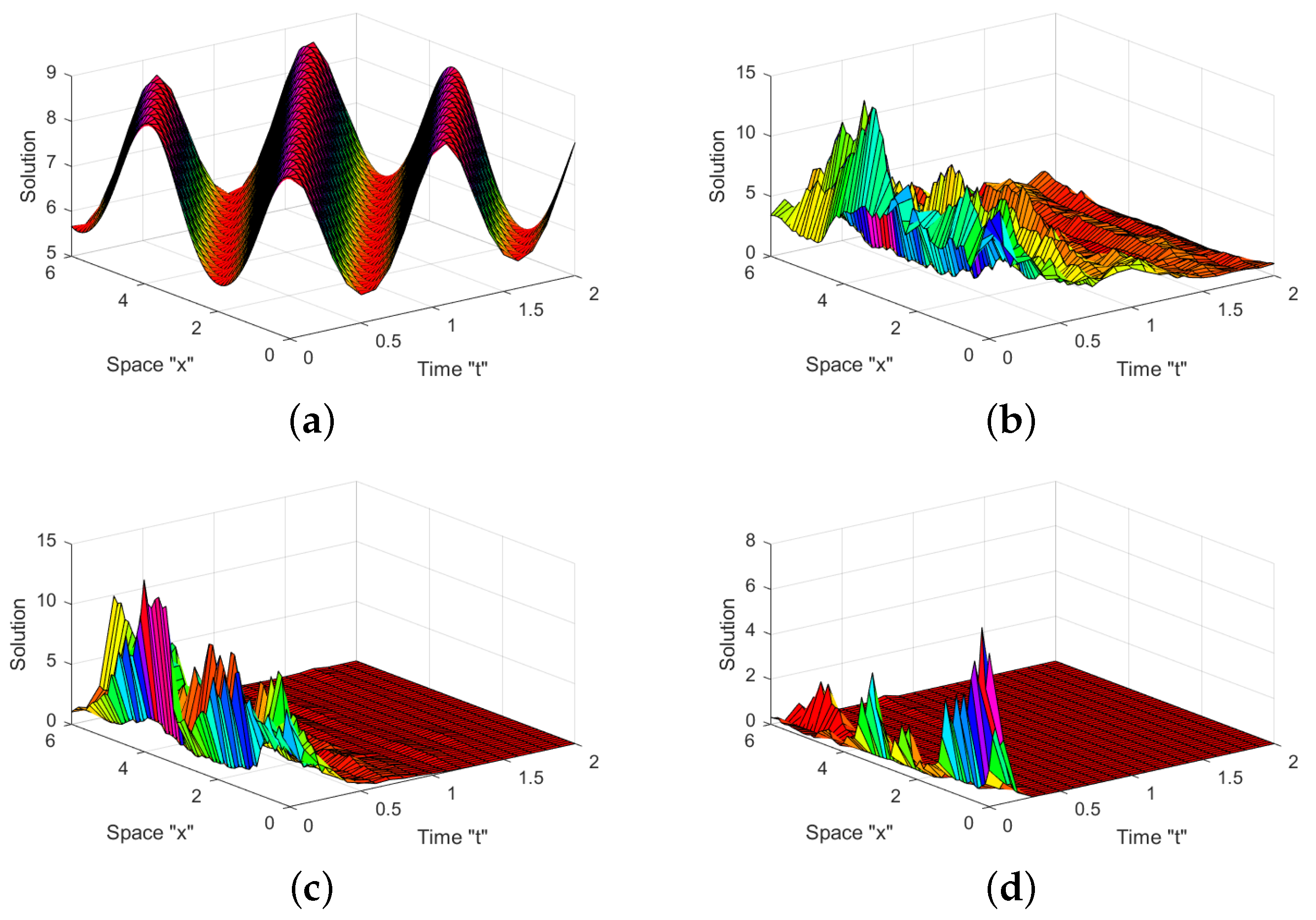
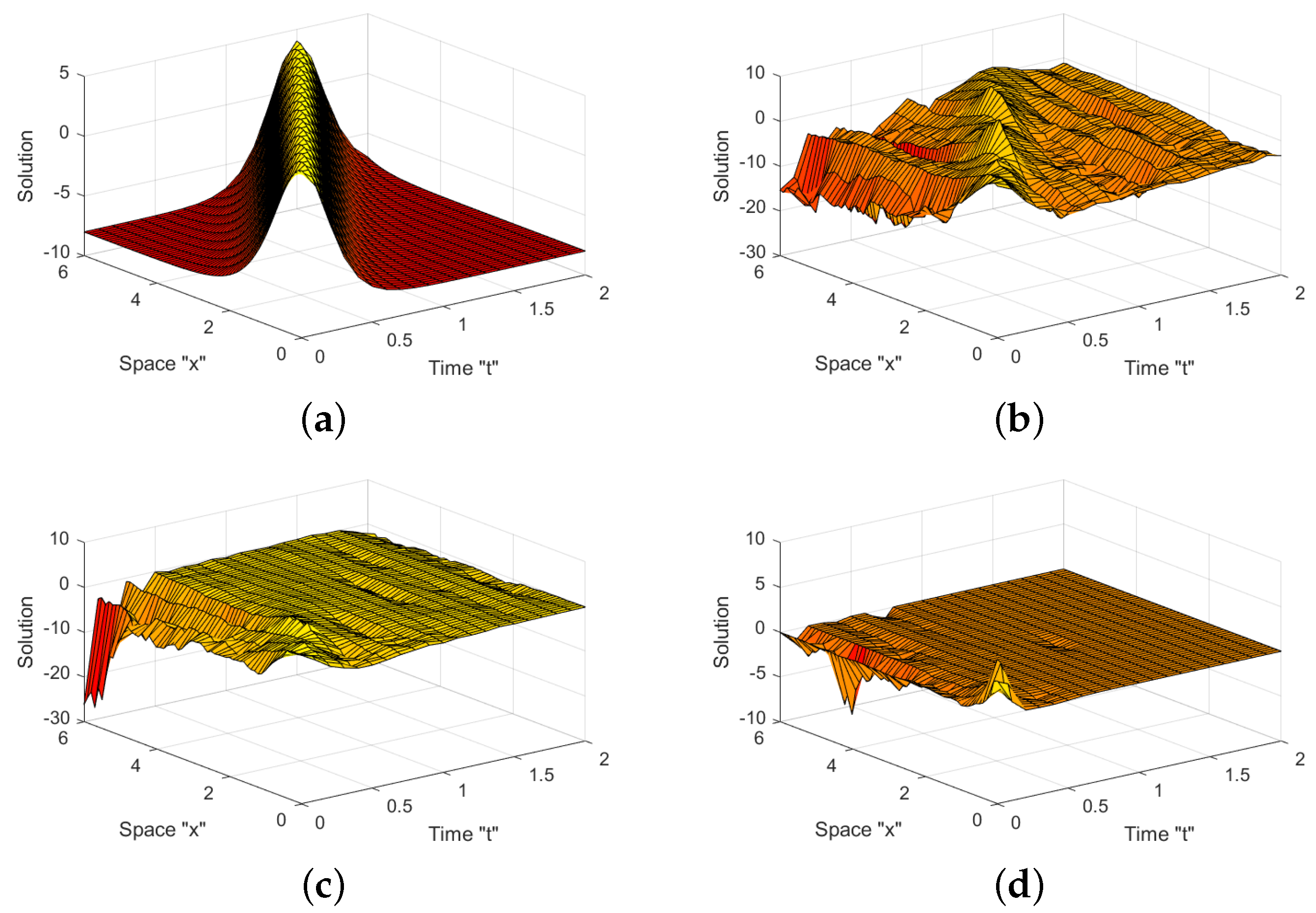
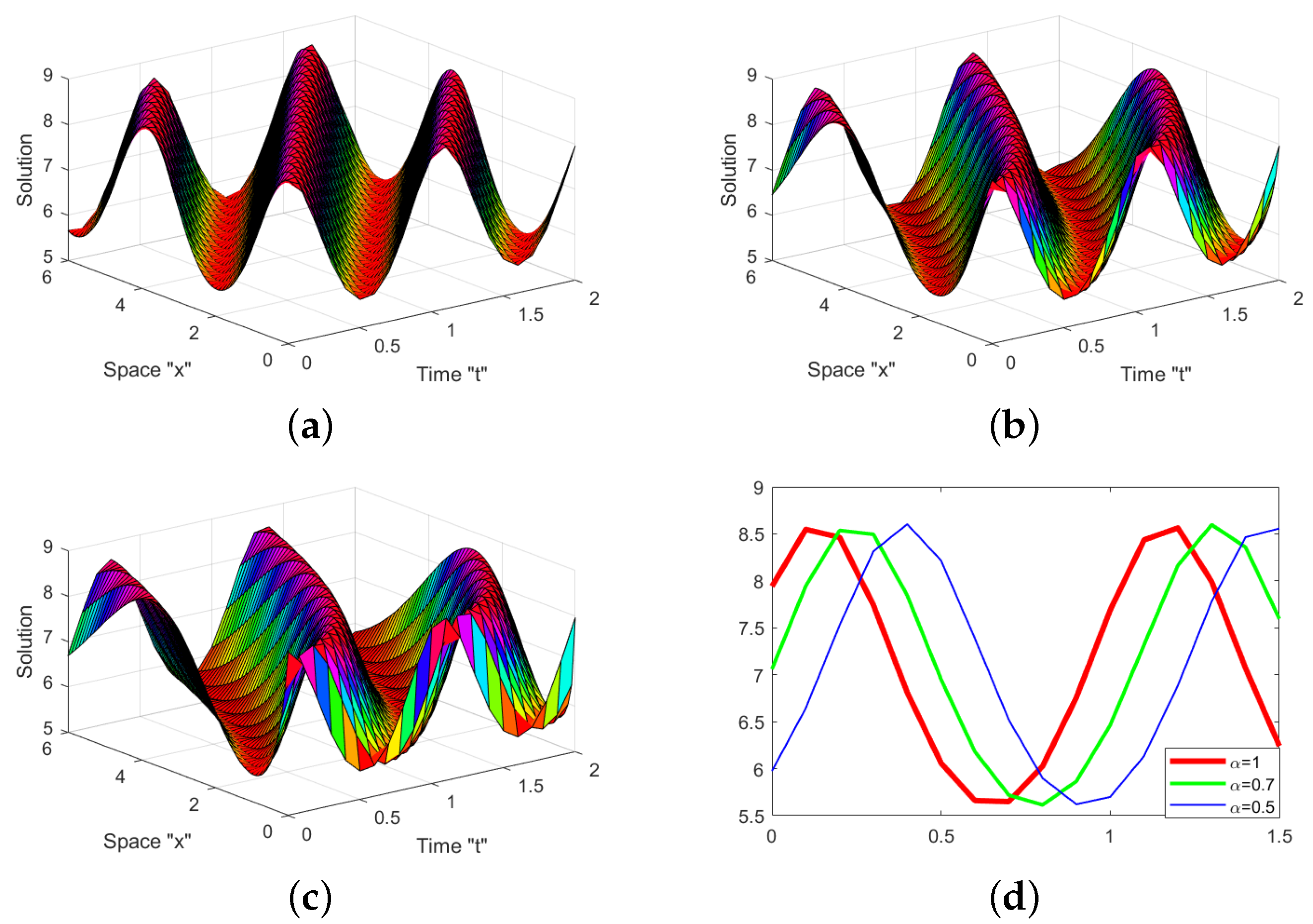
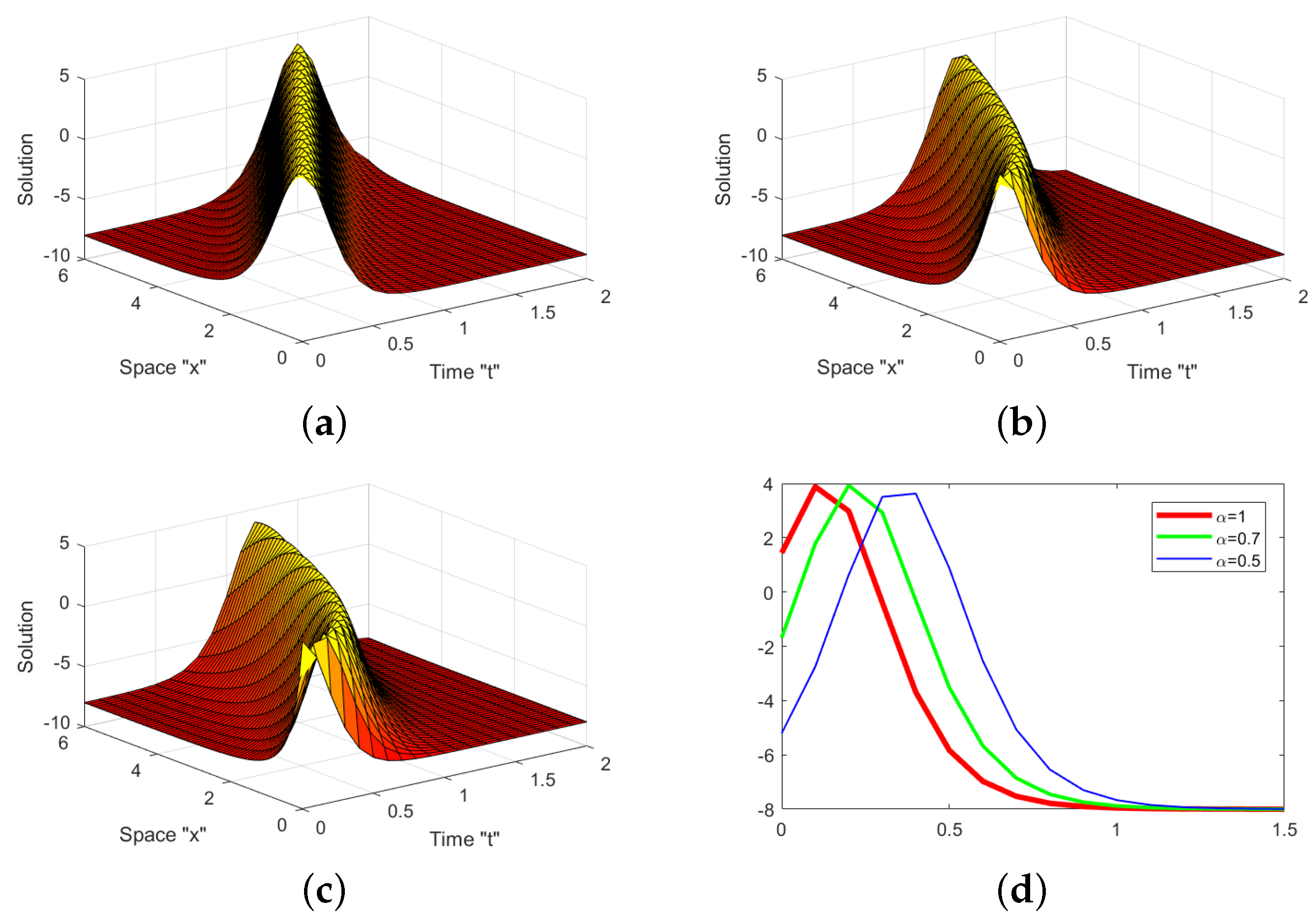
4. Graphical Representation and Discussion

In this paper, the analytical solutions of FSQZKE were acquired. Many analytic solutions to FSQZKE, such as trigonometric, rational, elliptic, and hyperbolic solutions, were attained using modified F-expansion method and Jacobi elliptic function method. The first method, the Jacobi elliptic function, provided us with various solutions in the type of hyperbolic, trigonometric, and rational. While the second method, modified F-expansion, provided us with a variety of elliptic solutions. We introduced some graphical representations of the solutions using the Matlab program to better understand their behavior and features. The behaviors of the attained solutions can be controlled by switching the values of the free parameters. Consequently, switching the parameter values changes the nature of the graph. To show how the graph of the obtained solutions is impacted by the stochastic term and the fractional order, let us fix the next parameters ${\eta }_1=1,$ ${\eta }_2=-1,$ ${\eta }_3=1,x\in [0,6]$, $t\in [0,2],y=z=1,A=1,B=0.5,C=0.25,$ ${\ell }_2=\frac{1}{2}$.

First the impact of stochastic term:

We may conclude, from Figure 1 and Figure 2, that there are several various sorts of solutions, including periodic solutions, dark solutions, and others, when the noise is disregarded (i.e., at $\sigma =0$). When noise is taken into account, the surface after minor transit patterns considerably flattens down and gains strength by $\sigma =1,2$. This indicates that the stochastic term affects the FSQZKE solutions and causes them to stabilize around zero.

Second the impact of fractional order:

Finally, from Figure 3 and Figure 4 we inferred that the curves do not overlap. Furthermore, the solutions shift to the left when the order of the M-truncated derivative increases.

5. Conclusions

In this paper, we looked at the (3 + 1)-dimensional fractional-stochastic quantum Zakharov–Kuznetsov Equation (2) with M-truncated derivative. We obtained the trigonometric, hyperbolic, elliptic, and rational fractional-stochastic solutions of FSQZKE (2) by using the Jacobi elliptic function method and the modified F-expansion method. Additionally, we generalized a few previous results, such as those in [43,48]. The discovered solutions are crucial for deriving a wide range of exciting and complex phenomena. The impact of the stochastic term and fractional derivative on the analytical solution of the FSQZKE (2) was demonstrated using the Matlab program. Finally, we demonstrated how the FSQZKE solutions are impacted by the stochastic term and M-truncated derivative. In future work, we can study FSQZKE (2) with additive noise or with color multiplicative noise.

References

1. Arnold, L. Random Dynamical Systems; Springer: Berlin/Heidelberg, Germany, 1998. [Google Scholar]
2. Imkeller, P.; Monahan, A.H. Conceptual stochastic climate models. Stoch. Dyn. 2002, 2, 311–326. [Google Scholar] [CrossRef] [Green Version]
3. Mohammed, W.W.; Blömker, D. Fast-diffusion limit for reaction-diffusion equations with multiplicative noise. Stoch. Anal. Appl. 2016, 34, 961–978. [Google Scholar] [CrossRef] [Green Version]
4. Metzler, R.; Klafter, J. The random walk’s guide to anomalous diffusion: A fractional dynamics approach. Phys. Rep. 2000, 339, 1–77. [Google Scholar] [CrossRef]
5. Alshammari, M.; Iqbal, N.; Mohammed, W.W.; Botmart, T. The solution of fractional-order system of KdV equations with exponential-decay kernel. Results Phys. 2022, 38, 105615. [Google Scholar] [CrossRef]
6. Ionescu, C.; Lopes, A.; Copot, D.; Machado, J.A.T.; Bates, J.H.T. The role of fractional calculus in modeling biological phenomena: A review. Commun. Nonlinear Sci. Numer. Simul. 2017, 51, 141–159. [Google Scholar] [CrossRef]
7. Riesz, M. L’intégrale de Riemann-Liouville et le Problème de Cauchy pour L’équation des ondes. Bull. Société Mathématique Fr. 1939, 67, 153–170. [Google Scholar] [CrossRef] [Green Version]
8. Wang, K.L.; Liu, S.Y. He’s fractional derivative and its application for fractional Fornberg-Whitham equation. Therm. Sci. 2016, 1, 54. [Google Scholar] [CrossRef]
9. Miller, S.; Ross, B. An Introduction to the Fractional Calculus and Fractional Differential Equations; Wiley: New York, NY, USA, 1993. [Google Scholar]
10. Caputo, M.; Fabrizio, M. A new definition of fractional differential without singular kernel. Prog. Fract. Differ. Appl. 2015, 1, 1–13. [Google Scholar]
11. Atangana, A.; Baleanu, D. New fractional derivatives with non-local and non-singular kernel. Theory and application to heat transfer model. Therm. Sci. 2016, 20, 763–769. [Google Scholar] [CrossRef] [Green Version]
12. Khalil, R.; Horani, M.A.; Yousef, A.; Sababheh, M. A new definition of fractional derivative. J. Comput. Appl. Math. 2014, 264, 65–70. [Google Scholar] [CrossRef]
13. Atangana, A.; Baleanu, D.; Alsaedi, A. New properties of conformable derivative. Open Math. 2015, 13, 889–898. [Google Scholar] [CrossRef]
14. Sousa, J.V.; de Oliveira, E.C. A new truncated Mfractional derivative type unifying some fractional derivative types with classical properties. Int. J. Anal. Appl. 2018, 16, 83–96. [Google Scholar]
15. Mainardi, F. On some properties of the Mittag-Leffler function Eα(-tα), completely monotone for t > 0 with 0 < α < 1. Discret. Contin. Dyn. Syst.-B 2014, 19, 2267–2278. [Google Scholar]
16. Hussain, A.; Jhangeer, A.; Abbas, N.; Khan, I.; Sherif, E.S.M. Optical solitons of fractional complex Ginzburg–Landau equation with conformable, beta, and M-truncated derivatives: A comparative study. Adv. Differ. Equ. 2020, 2020, 612. [Google Scholar] [CrossRef]
17. Yang, X.F.; Deng, Z.C.; Wei, Y. A Riccati-Bernoulli sub-ODE method for nonlinear partial differential equations and its application. Adv. Differ. Equ. 2015, 1, 117–133. [Google Scholar] [CrossRef] [Green Version]
18. Al-Askar, E.M.; Mohammed, W.W.; Albalahi, A.M.; El-Morshedy, M. The Impact of the Wiener process on the analytical solutions of the stochastic (2+ 1)-dimensional breaking soliton equation by using tanh–coth method. Mathematics 2022, 10, 817. [Google Scholar] [CrossRef]
19. Mohammed, W.W.; Alshammari, M.; Cesarano, C.; El-Morshedy, M. Brownian Motion Effects on the Stabilization of Stochastic Solutions to Fractional Diffusion Equations with Polynomials. Mathematics 2022, 10, 1458. [Google Scholar] [CrossRef]
20. Yan, Z.L. Abunbant families of Jacobi elliptic function solutions of the dimensional integrable Davey-Stewartson-type equation via a new method. Chaos Solitons Fractals 2003, 18, 299–309. [Google Scholar] [CrossRef]
21. Hirota, R. Exact solution of the Korteweg-de Vries equation for multiple collisions of solitons. Phys. Rev. Lett. 1971, 27, 1192–1194. [Google Scholar] [CrossRef]
22. Khan, K.; Akbar, M.A. The exp(-φ(ς))-expansion method for finding travelling wave solutions of Vakhnenko-Parkes equation. Int. J. Dyn. Syst. Differ. Equ. 2014, 5, 72–83. [Google Scholar]
23. Mohammed, W.W. Approximate solutions for stochastic time-fractional reaction–diffusion equations with multiplicative noise. Math. Methods Appl. Sci. 2021, 44, 2140–2157. [Google Scholar] [CrossRef]
24. Mohammed, W.W. Fast-diffusion limit for reaction–diffusion equations with degenerate multiplicative and additive noise. J. Dynamics Differ. Equ. 2021, 33, 577–592. [Google Scholar] [CrossRef]
25. Hashemi, M.S.; Bahrami, F.; Najafi, R. Lie symmetry analysis of steady-state fractional reaction-convection-diffusion equation. Optik 2017, 138, 240–249. [Google Scholar] [CrossRef]
26. Chu, Y.M.; Inc, M.; Hashemi, M.S.; Eshaghi, S. Analytical treatment of regularized Prabhakar fractional differential equations by invariant subspaces. Comp. Appl. Math. 2022, 41, 271. [Google Scholar] [CrossRef]
27. Wazwaz, A.M. A sine-cosine method for handling nonlinear wave equations. Math. Comput. Model. 2004, 40, 499–508. [Google Scholar] [CrossRef]
28. Yan, C. A simple transformation for nonlinear waves. Phys. Lett. A 1996, 224, 77–84. [Google Scholar] [CrossRef]
29. Seadawy, A.R.; Jun, W. Mathematical methods and solitary wave solutions of three-dimensional Zakharov-Kuznetsov-Burgers equation in dusty plasma and its applications. Results Phys. 2017, 7, 4269–4277. [Google Scholar]
30. Wang, M.L.; Li, X.Z.; Zhang, J.L. The (G/G)-expansion method and travelling wave solutions of nonlinear evolution equations in mathematical physics. Phys. Lett. A 2008, 372, 417–423. [Google Scholar] [CrossRef]
31. Zhang, H. New application of the (G/G)-expansion method. Commun. Nonlinear Sci. Numer. Simul. 2009, 14, 3220–3225. [Google Scholar] [CrossRef]
32. Foondun, M. Remarks on a fractional-time stochastic equation. Proc. Am. Math. Soc. 2021, 149, 2235–2247. [Google Scholar] [CrossRef] [Green Version]
33. Thach, T.N.; Kumar, D.; Luc, N.H.; Tuan, N.H. Existence and regularity results for stochastic fractional pseudo-parabolic equations driven by white noise. Discret. Contin. Dyn. Syst.-S 2022, 15, 481–499. [Google Scholar] [CrossRef]
34. Korpinar, Z.; Tchier, F.; Inc, M.; Bousbahi, F.; Tawfiq, F.M.O.; Akinlar, M.A. Applicability of time conformable derivative to Wick-fractional-stochastic PDEs. Alex. Eng. J. 2020, 59, 1485–1493. [Google Scholar] [CrossRef]
35. Mohammed, W.W.; Cesarano, C.; Al-Askar, F.M. Solutions to the (4+ 1)-Dimensional Time-Fractional Fokas Equation with M-Truncated Derivative. Mathematics 2022, 11, 194. [Google Scholar] [CrossRef]
36. Al-Askar, F.M.; Cesarano, C.; Mohammed, W.W. The Analytical Solutions of Stochastic-Fractional Drinfel’d-Sokolov-Wilson Equations via (G’/G)-Expansion Method. Symmetry 2022, 14, 2105. [Google Scholar] [CrossRef]
37. Al-Askar, F.M.; Mohammed, W.W. The analytical solutions of the stochastic fractional RKL equation via Jacobi elliptic function method. Adv. Math. Phys. 2022, 2022, 1534067. [Google Scholar] [CrossRef]
38. Alshammari, S.; Mohammed, W.W.; Samura, S.K.; Faleh, S. The analytical solutions for the stochastic-fractional Broer–Kaup equations. Math. Probl. Eng. 2022, 2022, 6895875. [Google Scholar] [CrossRef]
39. Moslem, W.M.; Ali, S.; Shukla, P.K.; Tang, X.Y. Rowlands: Solitary, explosive, and periodic solutions of the quantum Zakharov–Kuznetsov equation and its transverse instability. Phys. Plasmas 2007, 14, 082308. [Google Scholar] [CrossRef]
40. Washimi, H.; Taniuti, T. Propagation of ion-acoustic solitary waves of small amplitude. Phys. Rev. Lett. 1966, 17, 996–998. [Google Scholar] [CrossRef]
41. Mushtaq, A.; Shah, H.A. Nonlinear Zakharov–Kuznetsov equation for obliquely propagating two-dimensional ion-acoustic waves in a relativistic, rotating magnetized electron–positron–ion plasma. Phys. Plasmas 2005, 12, 072306. [Google Scholar] [CrossRef]
42. Qu, Q.X.; Tian, B.; Liu, W.J.; Sun, K.; Wang, P.; Jiang, Y.; Qin, B. Soliton solutions and interactions ofthe Zakharov-Kuznetsov equation in the electron-positron-ion plasmas. Eur. Phys. J. D 2011, 61, 709–715. [Google Scholar] [CrossRef]
43. Zayed, E.M.E.; Alurrfi, K.A.E. Extended generalized (G/G)-expansion method for solving the nonlinear quantum Zakharov–Kuznetsov equation. Ric. Mat. 2016, 65, 235–254. [Google Scholar] [CrossRef]
44. Zhang, C. Analytical and Numerical Solutions for the (3+1)-dimensional Extended Quantum Zakharov-Kuznetsov Equation. Appl. Comput. Math. 2022, 11, 74–80. [Google Scholar]
45. Zhang, B.; Liu, Z.; Xiaob, Q. New exact solitary wave and multiple soliton solutions of quantum Zakharov-Kuznetsov equation. Appl. Math. Comput. 2010, 217, 392–402. [Google Scholar] [CrossRef]
46. Ebadi, G.; Mojaver, A.; Milovic, D.; Johnson, S.; Biswas, A. Solitons and other solutions to the quantum Zakharov-Kuznetsov equation. Astrophys. Space Sci. 2012, 341, 507–513. [Google Scholar] [CrossRef]
47. Osman, M.S. Multi-soliton rational solutions for quantum Zakharov-Kuznetsov equation in quantum magnetoplasmas. Waves Random Complex Media 2016, 26, 434–443. [Google Scholar] [CrossRef]
48. Bhrawy, A.H.; Abdelkawy, M.A.; Kumar, S.; Johnson, S.; Biswas, A. Solitons and other solutions to quantum Zakharov–Kuznetsov equation in quantum magneto-plasmas. Indian J. Phys. 2013, 87, 455–463. [Google Scholar] [CrossRef]
49. Peng, Y.Z. Exact solutions for some nonlinear partial differential equations. Phys. Lett. A 2013, 314, 401–408. [Google Scholar] [CrossRef]
50. Zahrana, E.H.M.; Khater, M.M.A. Modified extended tanh-function method and its applications to the Bogoyavlenskii equation. Appl. Math. Model. 2016, 3, 1769–1775. [Google Scholar] [CrossRef]
Figure 1. For Equation (33), (ad) with k = 1 , α = 1 , β = 0 , λ = 4 , indicate the 3D profiles (a) σ = 0 (b) σ = 0.5 (c) σ = 1 and (d) σ = 2 .
Mathematics 11 00488 g001
Figure 2. For Equation (16), (ad) with m = 0.5 ,   α = 1 , β = 0 , λ = 13 , indicate the 3D profiles (a) σ = 0 (b) σ = 0.5 (c) σ = 1 and (d) σ = 2 .
Mathematics 11 00488 g002
Figure 3. For Equation (33), (ac) with parameters k = 1 , σ = 0 , λ = 4 ,indicate the 3D profiles and (d) denotes the 2D plot for different values of α at t = 1.5 and there is no overlap between the curves of the solution. (a) α = 1 , β = 0 (b) α = 0.7 , β = 0.9 and (c) α = 0.5 , β = 0.9 .
Mathematics 11 00488 g003
Figure 4. For Equation (16), (ac) with parameters m = 0.5 ,   σ = 0 , λ = 13 indicate the 3D profiles and (d) denotes the 2D plot for different values of α at t = 1.5 and there is no overlap between the curves of the solution. (a) α = 1 , β = 0 (b) α = 0.7 , β = 0.9 and (c) α = 0.5 , β = 0.9 .
Mathematics 11 00488 g004
Disclaimer/Publisher’s Note: The statements, opinions and data contained in all publications are solely those of the individual author(s) and contributor(s) and not of MDPI and/or the editor(s). MDPI and/or the editor(s) disclaim responsibility for any injury to people or property resulting from any ideas, methods, instructions or products referred to in the content.