A Graph Pointer Network-Based Multi-Objective Deep Reinforcement Learning Algorithm for Solving the Traveling Salesman Problem

Abstract

Traveling Salesman Problems (TSPs) have been a long-lasting interesting challenge to researchers in different areas. The difficulty of such problems scales up further when multiple objectives are considered concurrently. Plenty of work in evolutionary algorithms has been introduced to solve multi-objective TSPs with promising results, and the work in deep learning and reinforcement learning has been surging. This paper introduces a multi-objective deep graph pointer network-based reinforcement learning (MODGRL) algorithm for multi-objective TSPs. The MODGRL improves an earlier multi-objective deep reinforcement learning algorithm, called DRL-MOA, by utilizing a graph pointer network to learn the graphical structures of TSPs. Such improvements allow MODGRL to be trained on a small-scale TSP, but can find optimal solutions for large scale TSPs. NSGA-II, MOEA/D and SPEA2 are selected to compare with MODGRL and DRL-MOA. Hypervolume, spread and coverage over Pareto front (CPF) quality indicators were selected to assess the algorithms’ performance. In terms of the hypervolume indicator that represents the convergence and diversity of Pareto-frontiers, MODGRL outperformed all the competitors on the three well-known benchmark problems. Such findings proved that MODGRL, with the improved graph pointer network, indeed performed better, measured by the hypervolume indicator, than DRL-MOA and the three other evolutionary algorithms. MODGRL and DRL-MOA were comparable in the leading group, measured by the spread indicator. Although MODGRL performed better than DRL-MOA, both of them were just average regarding the evenness and diversity measured by the CPF indicator. Such findings remind that different performance indicators measure Pareto-frontiers from different perspectives. Choosing a well-accepted and suitable performance indicator to one’s experimental design is very critical, and may affect the conclusions. Three evolutionary algorithms were also experimented on with extra iterations, to validate whether extra iterations affected the performance. The results show that NSGA-II and SPEA2 were greatly improved measured by the Spread and CPF indicators. Such findings raise fairness concerns on algorithm comparisons using different fixed stopping criteria for different algorithms, which appeared in the DRL-MOA work and many others. Through these lessons, we concluded that MODGRL indeed performed better than DRL-MOA in terms of hypervolumne, and we also urge researchers on fair experimental designs and comparisons, in order to derive scientifically sound conclusions.

1. Introduction

Optimization has become a highly active research area. Different optimization techniques have been used around the world to solve a variety of problems. Machine learning [1], evolutionary algorithms [2] and reinforcement learning [3] have been used and researched widely. Reinforcement learning algorithms are mostly used in game development and to solve complex puzzles. Reinforcement learning is a form of trial-and-error learning where an agent acts upon an environment and learns to optimize a certain value through its actions. This form of trial-and-error learning and its computational usage was discussed significantly in the 1960s by several scientists including Minsky [4]. The term “Reinforcement Learning” was first used in several engineering papers published around the 1960s [3]. Reinforcement learning can be used to solve any optimization problem that can be represented by a Markov decision process [5].

Basic reinforcement learning algorithms also have a drawback when handling problems with large state spaces. Storing all the transition probabilities or Q-values for large state spaces requires a larger memory, and searching through the Q-table to find the respective Q-values carries a lot of overhead. To overcome these situations, reinforcement learning algorithms are often coupled with an artificial neural network (ANN) [6]. These algorithms are referred to as deep reinforcement learning algorithms. The purpose of this ANN is to learn the underlying Q-Table and approximate the Q-values. Many policy gradient-based reinforcement learning approaches rely on ANNs to function in this capacity. Advanced reinforcement learning algorithms such as actor–critic methods [7], in fact, utilize two ANNs. These two networks work in parallel, and keep improving the accuracy of each other through the learning process.

Most of the basic reinforcement learning algorithms are intended to be focused on finding optimal solutions to achieve a single goal, and would not perform adequately when involving multi-goal problems. However, most of the real-world optimization tasks involve a compromise between multiple objectives. As a result, multi-objective reinforcement learning problems and an algorithm called DRL-MOA [7] were introduced, and are being researched to increase the performance and capability of solving multi-objective problems. Improving further upon the existing work based on multi-objective reinforcement learning algorithms, new methods are currently being researched that utilize deep reinforcement learning methods that we referred to as multi-objective deep reinforcement learning algorithms.

Traveling Salesman Problems (TSPs) have been used for over several decades for testing and assessing the capabilities of novel algorithms used in the field of operations research, especially in the sub-field of combinatorial optimization. Along with the recent improvements to ANNs and the introduction of new kinds of ANNs that are capable of handling sequential and temporal data, the advantages of using multi-objective deep reinforcement learning algorithms that utilize these networks have increased, especially, when finding optimal solutions for multi-objective TSPs. By utilizing ANNs such as pointer networks [8], researchers were able to generalize multi-objective deep reinforcement learning algorithms so that they can be trained on a small-scale TSP (like a TSP with just 40 cities), but can find optimal solutions for large scale TSPs (with even more than 1000 cities). A summary of multi-objective deep reinforcement learning algorithms using different ANNs can be found in [9,10].

However, the pointer network used by DRL-MOA might be good at learning one dimensional linear structures of a TSP route. Learning the two dimensional graphical structure of a TSP could pose some challenges. Motivated by the recent developments in this field and the broad applications, in this paper we propose to improve DRL-MOA by adapting a graph neural network into DRL-MOA, in order to learn the graph structure of a TSP better. We present an algorithm, called multi-objective deep graph pointer network-based reinforcement learning (MODGRL), based on an improved graph pointer network mechanism [11] and a weighted sum method-based decomposition strategy [7]. A key objective of this paper is to prove that MODGRL is better in learning TSP, and performs better than DRL-MOA and selected evolutionary algorithms from [7]. MODGRL and DRL-MOA were compared with NSGA-II, MOEA/D and SPEA2. The resulting Pareto-frontiers were evaluated using three different quality indicators, namely, hypervolume, spread and coverage over Pareto front (CPF). The selected quality indicators assess different aspects of quality, which is very important, since a single quality indicator cannot measure all aspects successfully at once [12,13].

The main contributions of this work are:

• A novel algorithm called MODGRL is introduced, which integrates a graph neural network with DRL-MOA to learn the graphical structures of TSPs. It outperforms the same selected algorithms from [7] in terms of hypervolume indicator.
• MODGRL and other algorithms’ performance are assessed by hypervolume, spread and CPF indicators, to demonstrate the importance of suitable and sufficient quality indicator selection.
• Additional experiments with 8000 iterations are performed, to demonstrate potential pitfalls that may be overlooked by many researchers.
• The same additional experiments also demonstrate the importance of using a stopping criterion that can be applied to algorithms in different categories (e.g., maximum time budget) [14].

The rest of the paper is organized as follows. How related algorithms have been evolved to solve TSPs are summarized in Section 2. Section 3 describes the MODGRL architecture and the datasets and hyperparameters used for the experiments. The experimental results are covered in Section 4, followed by important findings and discussions in Section 5. Finally, the conclusion is presented in Section 6.

2. Related Work

Multi-objective optimization problems such as TSPs have been around for a few decades. Researchers have developed many solutions to solve this kind of optimization problem. Among these solutions, multi-objective evolutionary algorithms such as non-dominated sorting genetic algorithm (NSGA)-II [15], strength Pareto evolutionary algorithm (SPEA) [16], Pareto local search, genetic local search [2], ant colony optimization (ACO) [17] and donkey and smuggle optimization (DSO) [18] have been a remarkable success. Readers may find important work of this category in survey papers such as [19,20].

For TSP challenges using ANNs, the input and output sequences will have varied lengths from problem to problem. Thus, relying on a vanilla recurrent neural network (RNN) [21] for learning the input features and predicting the next value of the sequence will limit us to fixed size input sequences [8]. This will often require re-training of the models when the problem changes. By combining multiple RNNs, Sutskever et al. [22] introduced a more flexible network model that was capable of learning from varying length input sequences. In this model, separate RNNs were used as an encoder and a decoder. The decoder contained the attention mechanism, and was dependent only on the output of the encoder. The encoder used the varying length input sequences and generated a fixed length encoded vector. This allowed the network to handle inputs with varying lengths. Later, Bahdanau et al. [23] modified the decoder of the network from [22] by augmenting the network to propagate additional contextual information from the input sequence utilizing a content-based attention mechanism. Building further upon this, Vinyals et al. [8] introduced another attention-based model called the pointer network.

This pointer network [8] can overcome a key weakness that existed in many of the attention models, namely, its inability to handle varying inputs. The pointer network model could take input sequences with varying lengths, making it a highly valuable component in many areas. This network was able to point to the index of the input sequence rather than blending the encoded inputs to a context vector as in other attention models.

The pointer network model was improved by Q. Ma et al. [11] to develop an improved pointer network that can learn the structure and the context of graph structured inputs. This model, referred to as the graph pointer network (GPN) [11], was able to use a matrix representation of the TSP as a graph, and utilize an aggregation method to aggregate values from the neighboring nodes to help the GPN learn the context of the TSP better. Since a GPN is capable of aggregating the values of the neighboring nodes when updating a node value allowing the node to retain knowledge about the surrounding nodes, this model performs better at learning structured representations such as graphs. This algorithm was able to perform well when learning on the single-objective TSP and managed to outperform many of the existing single-objective TSP approaches [11].

Unlike the neural network models that rely on existing data to predict the next action, reinforcement learning algorithms learn to solve optimization problems via an agent that acts upon an environment. Thus, a reinforcement learning algorithm can adjust for changes in the environment (e.g., the addition of extra cities, change of city locations in the case of a TSP) and provide Pareto optimal solutions for it without the need to re-train. Although the number of researches conducted for multi-objective reinforcement learning on combinatorial optimization are still limited, many researches have been conducted on single-objective reinforcement learning algorithms and their ability to handle problems such as TSPs and Deep-Sea Treasure [6,24]. These researches show that reinforcement learning can perform as well as the other existing methods and even outperform them. As a result, there are plenty of examples and simulation/testing training frameworks built to handle single-objective TSPs.

However, when trying to solve multi-objective optimization problems using reinforcement learning, the most common approach is to rely on a scalarization function. Following this approach, many of the multi-objective reinforcement learning and multi-objective deep reinforcement learning algorithms utilize a scalarization function where the multiple objectives are assigned different priorities, and use it to generate a single scalarized function after computing the reward vector [7,9]. More recent papers using multi-objective deep reinforcement learning approaches (e.g., DRL-MOA in [7]) utilized weighted sum method-based decomposition strategies, where the main multi-objective optimization problem was broken down into several scalarized optimization problems. Based on this decomposition strategy, by solving the subproblems and finding the respective Pareto-optimal solutions, the DRL-MOA was able to obtain the Pareto-frontier.

Furthermore, DRL-MOA [7] combined the decomposition strategy and used an actor–critic reinforcement learning algorithm [25,26], to solve each of the sub-problems effectively to generate the Pareto frontier. Actor–critic algorithms are a combination of actor-only methods such as policy gradient and critic-only methods such as temporal difference learning [26]. The actor behaves as the policy generation mechanism, while the critic can be considered as the value function. The actor can be augmented with any ANN or policy gradient method, while the critic can be augmented with any policy evaluation method that is used commonly, or by using an ANN. This enables the researchers to develop actor–critic algorithms to benefit from the ANNs, as well as the advantages provided by the reinforcement learning algorithms.

Based on the analysis of the most recent related work presented above, it is evident that there is a lot of research using reinforcement learning algorithms for single-objective traveling salesman problems, and many more new research are emerging to evaluate the capability of reinforcement learning algorithms to solve multi-objective traveling salesman problems. Some of these new research algorithms utilize the state-of-the-art graph-based artificial neural networks [10] to solve single-objective TSPs. By improving upon the recent developments, we believe that by leveraging the power of graph-based neural networks, multi-objective deep reinforcement learning algorithms could be improved further and solve multi-objective TSPs more efficiently. With such, the multi-objective deep graph pointer network-based reinforcement learning (MODGRL) is introduced in Section 3.

Since DRL-MOA [7] was introduced, there has been some related work applying multi-objective deep reinforcement learning to other combinatorial optimization problems. For example, in [27], a pointer network-based multi-objective deep reinforcement learning model was introduced to assist service function chains placement needed for 5G (or beyond) network services’ strict quality of service requirements (e.g., minimizing E2E latency and minimizing computing resource congestion among all nodes). In [28], a deep Q-network-based multi-objective deep reinforcement learning model was introduced to recommend movies based on three conflicting metrics, namely, precision, novelty, and diversity. MODRL/D-EL [29] introduced a hybrid solution to improve MODRL/D-AM from [30], and a new evolutionary learning model to solve a multi-objective vehicle routing problem with time windows (MO-VRPTW) [29]. There are also some related works dedicated to scheduling problems for different domains (e.g., [31,32,33]) or utilized deep learning solutions or reinforcement learning solutions, rather than both, listed in [34], to solve multi-objective TSPs. Yet, to the best of our knowledge, our work is the only multi-objective model with both deep learning and reinforcement learning, and is specifically for solving multi-objective TSPs after DRL-MOA, MODRL/D-AM [30] and Ouyang’s work in [34] were introduced. Since there was no source code of [30,34] available at the time of our experiments, we did not include these two for fair comparison purposes [14,35]. We suggest readers refer to their work and experimental results in [30,34].

3. Multi-Objective Deep Graph Pointer Based Reinforcement Learning

This section first reviews traveling salesman problems in Section 3.1, and then introduces the datasets and hyperparameters for MODGRL in Section 3.2 and Section 3.3. The model architecture of MODGRL is then presented in the following subsections from Section 3.4, Section 3.5, Section 3.6 and Section 3.7.

3.1. Traveling Salesman Problems

A TSP is an NP-hard problem where the objective is to find a tour that allows the salesman to start from some city and visit all other cities and return to the origin. A single-objective TSP attempts to find the optimal tour by minimizing the distance travelled [36]. However, in many real world scenarios, we often have to optimize more than one objective. A bi-objective TSP (BOTSP) is a variant of TSPs where each edge will contain two independent cost values. The objective of a BOTSP solver is to find the tour that would minimize both cost functions. For a BOTSP with N cities, the costs for two objectives can be denoted, respectively, as $c_{ij}^1$ and $c_{ij}^2$, where $i,j=1,2,3\dots N$, representing the costs for moving from city i to city j. In a Euclidean TSP example from [37], the two costs are usually the distance between the coordinates of the two cities. In [38], the multi-objective optimization problem with variable travel time example could have travel distance and travel time as two cost objectives. Therefore, for a BOTSP, each city requires to have two sets of coordinates, each of which correspond to a different objective. As the two costs $c_{ij}^1$ and $c_{ij}^2$ are independent and often conflicting, the final solution will be a set of Pareto-optimal solutions. A BOTSP can be defined mathematically as follows [19]:

$$“min”z_k\left(\rho \right)=\sum _{i=1}^{N-1}{c}_{\rho \left(i\right),\rho (i+1)}^k+c_{\rho \left(N\right),\rho \left(1\right)}^k,k=1,\dots ,p.$$

(1)

where $\rho$ represents a cyclic permutation of the N cities. When $p=2$, the equation is expressed as a BOTSP; and when $p>2$, the equation is generalized as a multi-objective TSP.

TSPLIB [39] provides a collection of test cases that contain many TSPs, including single-objective and multi-objective TSPs. It is generally used as a standard test set to benchmark TSP solvers.

3.2. Training and Validation datasets

We are training the model using a set of randomly generated bi-objective Euclidean TSPs with 40 cities. Each problem consists of 40 cities, and each city contains two sets of independent coordinate points $\left[\right[x1,y1\left]\right[x2,y2\left]\right]$ in the euclidean space. Each coordinate pair represents the values associated with the corresponding objective. The training set was generated using the random generator from the pytorch library using the seed value 12,345. The training set contained 500,000 samples, each with 40 cities, and each city had two pairs or Euclidean coordinates between $[0,1]$. The validation dataset contained 1000 samples, and was generated following the same procedure as the training set using the seed value 12,346 instead.

3.3. Hyperparameters

For this project we used a batch size of 200 and a learning rate of 0.05. The learning rate is decayed by a factor of 0.0005 after every 10,000 samples. We also utilized the pre-training approach [7], using five episodes for the first sub-problem and three episodes for every sub-problem after the initial one. This is because we are reusing the weight values of the GPN obtained for the previous set of weight configurations for the next set as the initial values, thereby speeding up the training process.

3.4. Model

In our implementation of the MODGRL algorithm, we follow the approaches presented in two very recent papers [7,11] that performed well in their respective problem domains. There are three main components in the MODGRL algorithm:

• The decomposition strategy,
• Self-critic reinforcement learning agent,
• Graph pointer network for approximations.

The decomposition strategy acts as the outer loop of the MODGRL algorithm and handles the decomposition of the multi-objective optimization problem into a set of scalar optimization problems. Each of the sub problems is handled by the reinforcement learning agent. This reinforcement learning agent makes use of the graph pointer network to generate the TSP tours and evaluate them. Based on the calculated loss after the evaluation, the reinforcement learning agent updates the weights of the graph pointer network making it more accurate over time.

3.5. The Decomposition Strategy

We follow the decomposition strategy presented by [7]. This project utilizes the widely used weighted sum approach when decomposing the multi-objective optimization (MOO) problem into a set of scalarized optimization problems. Solving these scalarized functions will generate the Pareto optimal solution for the MOO problem. Assuming we have N scalar optimization subproblems and M objectives, our weight vector can be represented as $w_{ij}$ = $[[w_{11},w_{12},w_{1M}],\dots ,[w_{N1},w_{N2},w_{NM}]].$

For the bi-objective TSP, assume M = 2 and we have N = 101 subproblems. By using the weighted sum approach, we split the problem into 101 scalar optimization problems, each containing a weight vector corresponding to the two objectives. To split, we initialize a weight vector as $w_{ij}$ = $\left[\right[0,1.0],[0.01,0.99],[0.02,0.98],\dots ,[0.98,0.02],[0.99,0.01],[1.0,0\left]\right]$ [7,30].

Thus, for each scalarized subproblem $w_i$, there will be two weight values $w_{i1}$ and $w_{i2}$, each corresponding to the two objectives of the bi-objective TSP and the sum of the weights is equal to 1. Thus, we obtain the outermost loop for the proposed MODGRL algorithm, which iterates over the entire weight vector from $i=0$ until $i=N$ [30].

For each subproblem, the reward function is modeled using two weight values and the corresponding reward values for each of the two objectives. Thus, for the reward function R for the ith subproblem could be calculated with Equation (2), where $f_1\left(x\right)$ and $f_2\left(x\right)$ represent the corresponding reward values for each objective and x is the obtained tour. The goal of the MODGRL algorithm is to minimize $R_i\left(x\right)$ for $0\le i\le N$, see [7]

$$R_{i\left(x\right)}=(w_{i1}\ast f_{1\left(x\right)}+w_{i2}\ast f_{2\left(x\right)}).$$

(2)

3.6. Self-Critic Reinforcement Learning Agent

This paper uses the self-critic architecture utilized by [7]. The self-critic model used by Kaiwen Li et al. is a modified variant of the actor–critic reinforcement learning architecture. The actor–critic models were developed from the gradient descent methods and were designed as a hybrid model to take advantage of both policy-based and value-based reinforcement learning methods. Generally, in an actor–critic model there are two main components.

3.6.1. Actor

The actor handles the generation of the policy and then decides where the agent should move to. In the case of a TSP, the actor is what generates the tour for the given TSP.

3.6.2. Critic

A critic uses a value-based approach and evaluates the actions taken by the agent. In the TSP context, once the actor generates the tour, a critic will take in the tour and give a value for the tour. This value can be used as the approximation when calculating the loss function to update the weights of both the networks.

The self critic method only uses a single artificial neural network model instead of the usual two actor and critic models. In this architecture, the ANN functions both as the actor and the critic. When functioning as the actor, the agent will choose the next city to visit at random from the probability distribution generated by the model. The model in this case will return the generated tour and the probability distribution for selecting the next city.

When the model needs to function as the critic, instead of choosing the next city to visit randomly, the agent selects the city with the highest probability ($prob$), and produces the total distance of the tours as the reward values ($R1$ and $R2$). This strategy generates two different tours ($t1$ and $t2$), obtained using the same ANN, one generated at random and the other, the best possible tour. The reward value from the best possible tour ($R1$) is used as the approximation of what the reward value should be, and the $loss$ is calculated based on the two reward values $R1$ and $R2$. The generated loss is used to update the weights of the model.

The high-level architecture of the proposed MODGRL algorithm can be explained by the pseudo-code given below.

Listing 1. The MODGRL Algorithm.

for w1,w2 in W:

for i in range(0,e):

for b in T:

t1,R1,prob = Actor()

t2, R2 = Critic()

loss = R1 - R2

loss.backwards()

save_model()

W is the set of weights the sub problems generated using the weighted sum based decomposing strategy described in Section 3.5. $w_1$ and $w_2$ represent the respective weights for the two objectives. The algorithm loops over each epoch i until the predetermined number of epochs, e, is reached. b is a single batch, and T is the list containing all the batches. The decomposition strategy acts as the controller of the MODGRL algorithm, allowing the algorithm to loop over all the subproblems, as described in Section 3.5.

3.7. Graph Pointer Network for Approximations

The GPN used in the MODGRL algorithm was adapted from the work presented by [11]. Their algorithm was designed for solving single-objective optimization problems and performed well in their problem space. We adapted this algorithm for our bi-objective MODGRL algorithm by making the necessary changes to the input vectors and the respective components.

For this specific project, by using a GPN architecture, we developed a Reinforcement Learning agent that can be trained on small scale multi-objective TSPs with about 20 or 40 cities, and used that same trained model to predict large scale multi-objective TSPs with 100 or more cities. In fact, Ref. [11] used this GPN approach which allows their model to train on small scale single-objective TSPs (with 20, 40 cities) and then to solve large scale single-objective TSPs (with 100, 200, 500 cities). The MODGRL algorithm also shows such scalability when being applied to multi-objective TSPs. This is a huge advantage, as the training time needed for large scale multi-objective TSPs is very long, and by training the agent on small scale problems we can reduce it by more than a half. This is because, if we were to train the algorithm with a 100 city problem, each tour would have 100 cities, whereas, if we train on a problem with just 20 or 40 cities, each tour would only contain 20 or 40 cities, respectively.

Figure 1 presents the data flow and control flow of the algorithms, and how each of the different components are integrated and function.

Table 1. The components of the GPN and its functionality. x refers to the number of cities in the TSP and y refers to the number of parameters in the objective. In the bi-objective Euclidean TSP, there are two objectives. Each objective is made up of 2 parameters to represent the coordinates of the location.

Component	Functionality	Network Type	Input	Output
Embedder 1	Embed all the coordinates values of all the cities in the entire problem.	Linear Layer	Vector containing all city coordinates $[x,2\ast y]$.	Vector of size $[x,128]$.
Embedder 2	Embed the coordinate values of the current city.	Linear Layer	Vector containing current city coordinates $[1,2\ast y]$.	Vector of size $[1,128]$.
Encoder 1	Use the output from Embedder 1 and aggregate the neighboring values to capture the entire graph.	Graph Encoder	Output from Embedder 1.	Encoded representation of the cities of size x
Encoder 2	Use the output from Embedder 1 to capture information related to the sequence of visited cities.	LSTM	Output from Embedder 2, Previous cell gate value, Previous output gate value.	Output gate value, cell gate value.

summarizes how the components in Figure 1 are structured, and the inputs and outputs of each of the different components, and what the component is, along with their functionality/usage. In Figure 1 and Table 1, the two embedders are responsible for embedding the graph matrix and the current city value. The embedded current city value is then passed on to the long-short-term memory (LSTM) to be encoded. The embedded graph structure is passed on to the graph encoding/aggregation layers. The outputs from the two encoders are used as the input for the final pointer. This layer will generate the final probability distribution for selecting the next city by generating the matrix-to-matrix product of the two encoded inputs and passing it through a SoftMax function. Additionally, x refers to the number of cities and y represents the number of objectives in Table 1. The number of objectives are multiplied by 2 every time, because each objective in our Euclidean TSP consists of a pair of coordinates to mark the location.

4. Experiments and Results

In order to replicate the experimental setting of [7], this paper selected DRL-MOA and two evolutionary algorithms (i.e., NSGA-II and MOEA/D) from [7] to compare with MODGRL. Additionally, SPEA2 was selected so that there were sufficient algorithms to conduct statistical analysis and rankings by CRS4EAs, “a novel method for comparing evolutionary algorithms, which evaluates and ranks algorithms regarding the formula from the Glicko-2 chess rating system [40]”. CRS4EAs [40,41] is capable of conducting non-parametric statistical tests [42]. An algorithm’s ranking is represented as an absolute rating value, meaning the absolute power of an algorithm after a tournament. Rating deviation and rating volatility, respectively, represent the range of a ranking based on a certain confidence interval (e.g., 95%) and the degree of expected fluctuation in a player’s rating. When two algorithms’ ranking ranges do overlap, it means these two algorithms are not statistically significant. Per [41], its statistical results are comparable with null hypothesis significance testing (NHST), which is “a method of statistical inference by which an experimental factor is tested against a hypothesis of no effect or no relationship, based on a given observation [43]”. CRS4EAs is also less sensitive to the number of problems, number of algorithms, and number of independent runs [41]. We first introduce the experimental settings of all the algorithms in Section 4.1, followed by the training and testing sets for the algorithms in Section 4.2. Finally, the experimental results are presented in Section 4.3, and assessed using three quality indicators.

4.1. Parameter Settings

For the two reinforcement learning algorithms, i.e., MODGRL and DRL-MOA, the hyperparameters were set the same and are described in Section 3.3. For all the selected evolutionary algorithms, i.e., NSGA-II, MOEA/D and SPEA2, the population size was set to 100, and each experiment was run 10 times.

4.2. Training and Testing Datasets

The training set was described in Section 3.2. For the testing dataset, commonly used KroAB 100, 150, and 200 instances were adopted, obtained from TSPLIB [39]. KroA and KroB are both used for testing single-objective traveling salesman problems. These datasets consist of Euclidean coordinates for each city. The Euclidean distance calculated from these coordinates is used as the object value, and needs to be minimized to satisfy the conditions of the TSP. By combining both KroA and KroB, researchers have created the KroAB datasets, which consists of two pairs of coordinates for each city. These two pairs are used as the two respective objectives for the bi-objective TSP. Since the two objectives are independent, optimizing one objective does not necessarily optimize the second objective. Thus, it makes the KroAB datasets ideal for testing bi-objective Euclidean TSP agents.

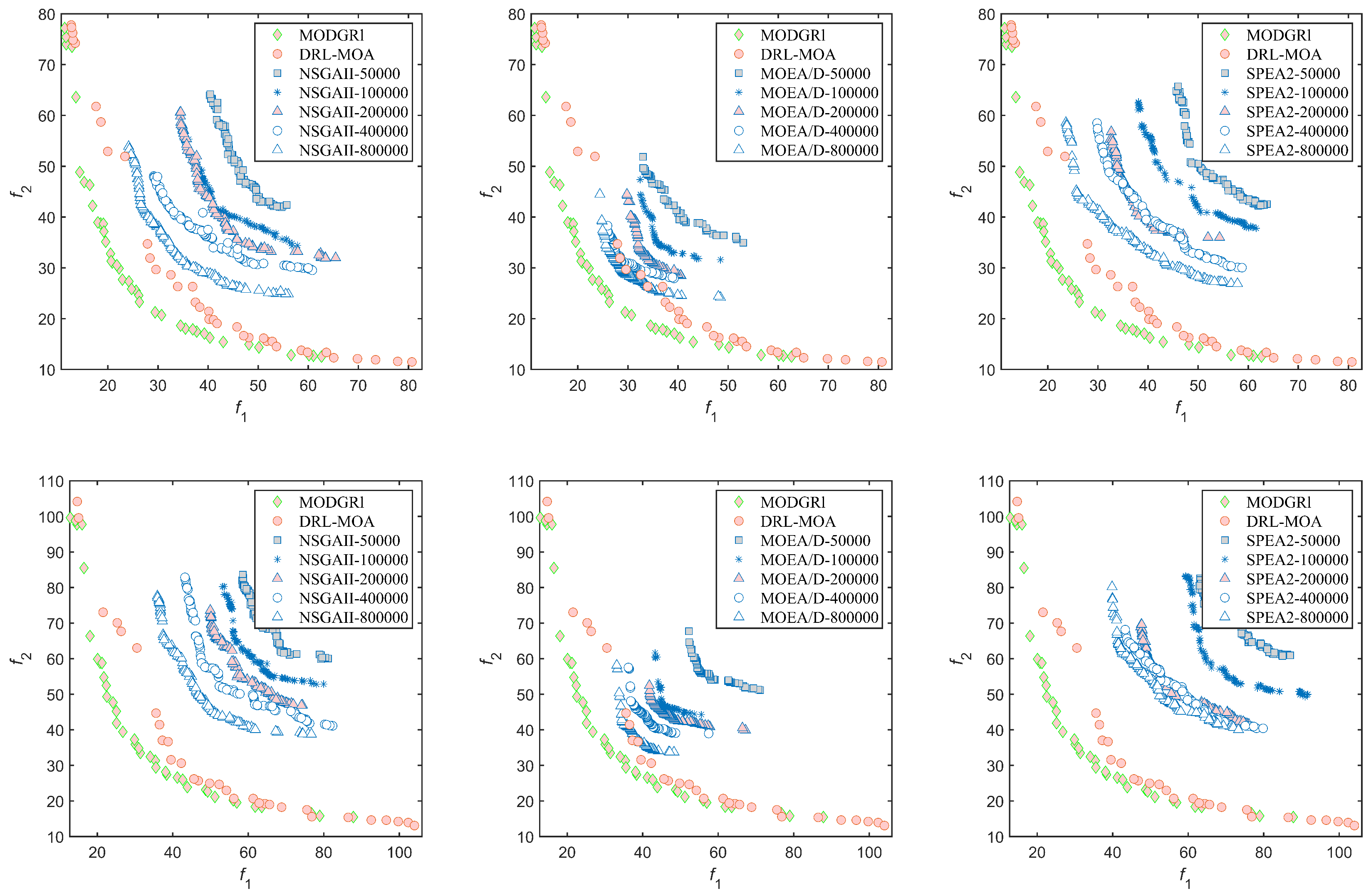
4.3. Experimental Results

In order to provide fair comparisons, the same experimental settings as in [7] were set for the selected evolutionary algorithms, which were terminated at 500, 1000, 2000, and 4000 iterations, and are equivalent to 50,000, 100,000, 200,000, and 400,000 fitness evaluations, respectively. Experiments of NSGA-II, MOEA/D and SPEA2 running with 800,000 fitness evaluations were also added, to observe whether doubling the fitness evaluations to 800,000 made the algorithms perform better or worse than MODGRL and DRL-MOA. Such extra experiments were performed to express the importance of algorithm comparisons under fair conditions, no matter if these algorithms are within the same or different categories.

First, since there are 17 Pareto-frontiers, we displayed the Pareto-frontiers of the KroAB 100 dataset in three separate plots in Figure 2, categorized by three different EAs, for better representations. Similar Pareto-frontiers of the KroAB 150 and 200 datasets are presented in the Appendix. As can be observed from the Figures, MODGRL’s Pareto-frontiers are much better than those of NSGA-II, MOEA/D, and SPEA2. The MOEA/D result running with 8000 iterations (equivalent to 800,000 fitness evaluations) shown in Figure 2 (middle), overlaps slightly with the result of MODGRL. Such an observation shows a good example of the need to use a quality indicator to measure algorithms’ performances, described in the next paragraph. Readers may also find that the Pareto-frontiers of MODGRL are also better than that of DRL-MOA in these Figures.

In order to analyze our experiments further, we computed the Pareto-frontiers of all the algorithms using three different quality indicators, namely, hypervolume [44], spread [45,46], and coverage over the Pareto front (CPF) [47]. The hypervolume indicator calculates the hypervolume of the area covered by a solution set with respect to a reference point. The value indicates a multi-objective algorithm’s performance on its Pareto-frontiers in terms of both convergence and diversity [47]. The Spread indicator ($\Delta$) was formulated in [15] to measure the diversity of Pareto-frontiers of bi-objective problems. Later, it was extended for those problems with more than two objectives [45,48]. Coverage over Pareto front (CPF) [47] is a newer indicator to assess both evenness and spread more accurately. All the experimental results are tabulated in Appendix A. Note that the hypervolume indicator is the only one used in [7]. Additionally, the indicator experimental results were analyzed statistically and ranked using CRS4EAs [40]. Because the MODGRL and DRL-MOA experiments were run 10 times with the average and standard deviation of the three indicators available, CRS4EAs is applicable to rank all the algorithms here. Note that there are no equivalent concepts of populations’ size and iterations available in deep reinforcement learning algorithms. For fairness comparison reasons [35], readers should be reminded that such inequivalences should be considered as threats of validity. We will discuss the fairness comparison with more details using our findings in Section 5.

Figure 3 shows that, regarding the KroAB100 dataset, both MODGRL and DRL-MOA were statistically significantly better than NSGA-II, MOEA/D, and SPEA2 with 4000 or fewer iterations. Such results also proved that our experiment was conducted comparably with the one in [7]. As for the three evolutionary algorithms running 8000 iterations, MODGRL outperformed all of them as well as DRL-MOA, but the differences were not significant except for SPEA2-80000. From Figure 4, we observed that MODGRL, DRL-MOA, NSGAII-800000 and SPEA2-800000 were in the leading group for all the datasets. Additionally, MODRGL and DRL-MOA were quite comparable, although NSGAII-800000 and SPEA2-800000 had larger rating score margins with MODGRL and DRL-MOA for the KroAB 100 dataset. In Figure 5, we can observe that MODGRL ranked first, excluding those with 8000 iterations, but there was no statistical significance with NSGAII-400000 and SPEA2-400000. For the KroAB150 and KroAB200 datasets, the rankings of the hypervolume, Spread and CPF indicators were very similar to those in Figure 3, Figure 4 and Figure 5. We put these figures in Appendix A.

Based on the obtained results from the three datasets, it is evident that MODGRL outperformed all the other compared algorithms in terms of convergence and diversity represented by the hypervolume indicator. MODGRL also performed relatively well in terms of evenness and spread of Pareto-frontiers measured by the Spread and CPF indicators. Lastly, MODGRL ranked better than DRL-MOA, although not all necessarilly statistical significant, for all but two results (i.e., KroAB 150 and KroAB 200 datasets measured by the Spread indicator shown in Appendix A) using the three quality indicators.

5. Discussions

There are several findings observed from the previous section that are worth further discussions, which could become good references for future research. All the findings are derived from the results of statistical analysis and rankings conducted by CRS4EAs.

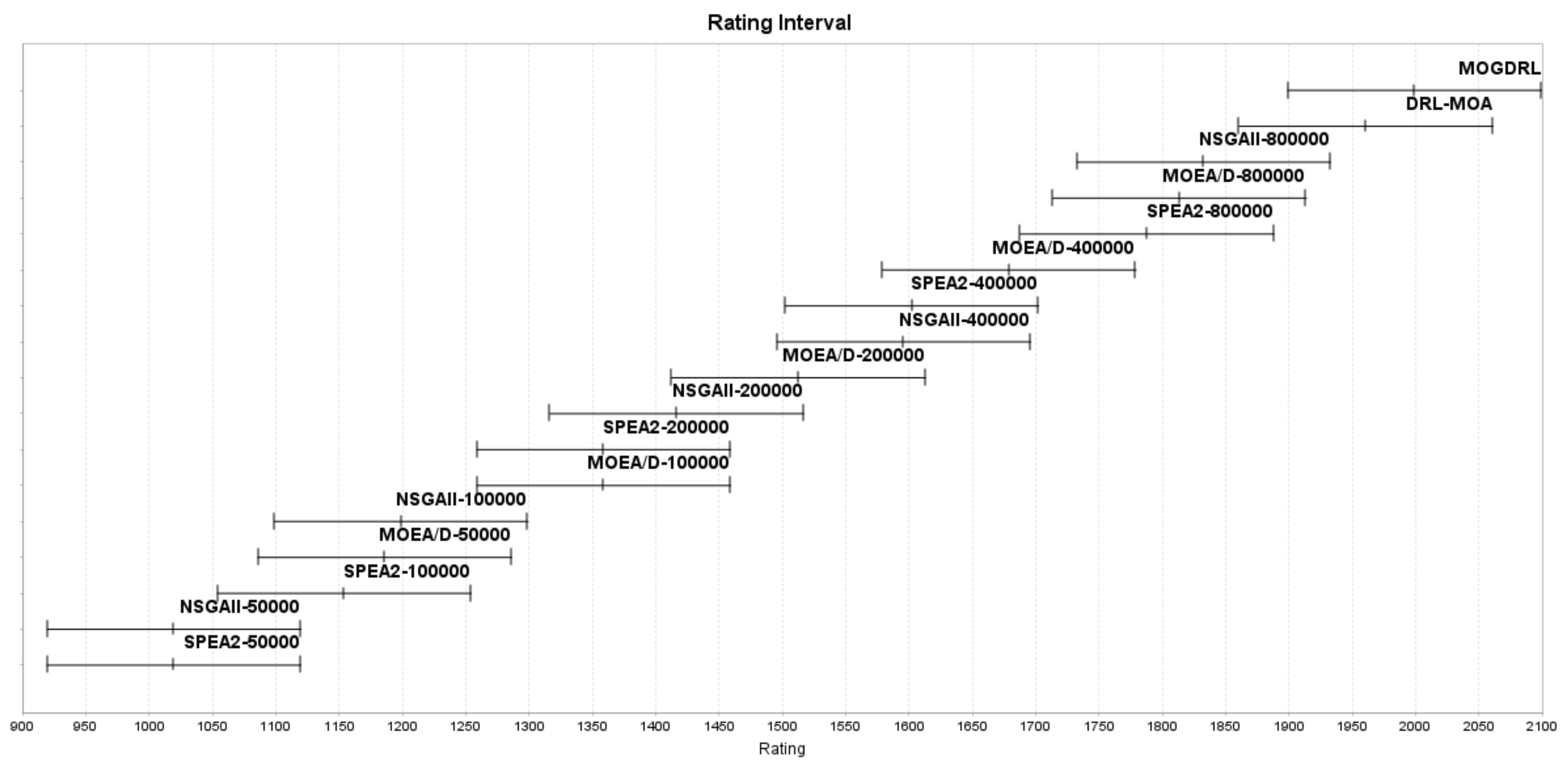
• Quality indicators: Although MODGRL stands out in terms of the hypervolume indicator for all the datasets, its CPF performance was only average between all the 17 competitors. Many researchers have discussed the applicability and advantages of different quality indicators for multi-objective optimization problems (e.g., [49]). As multi-objective deep reinforcement learning is emerging, utilizing suitable and multiple quality indicators is a must, so that the algorithms’ performances in different perspectives can be examined more thoroughly.
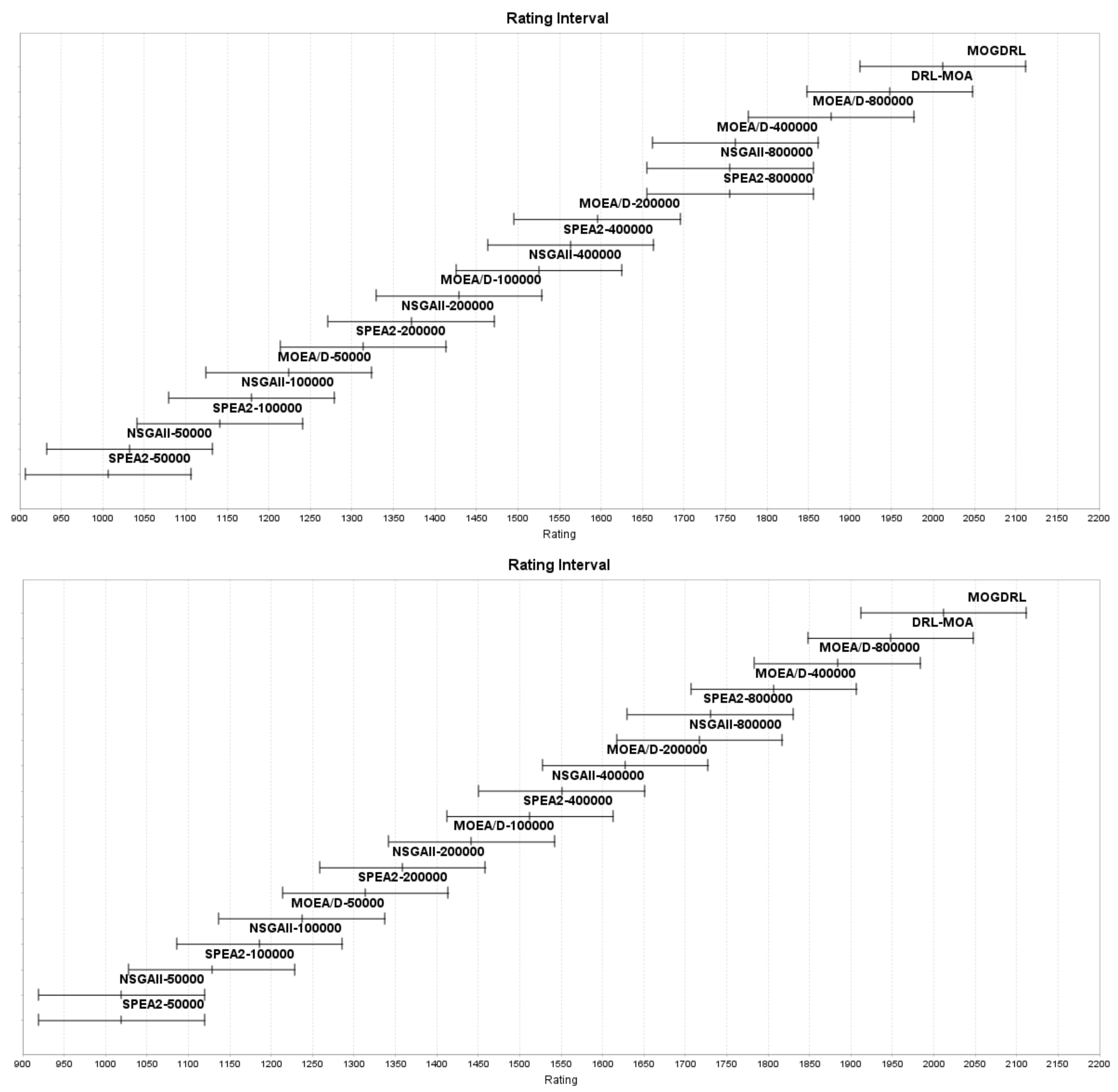
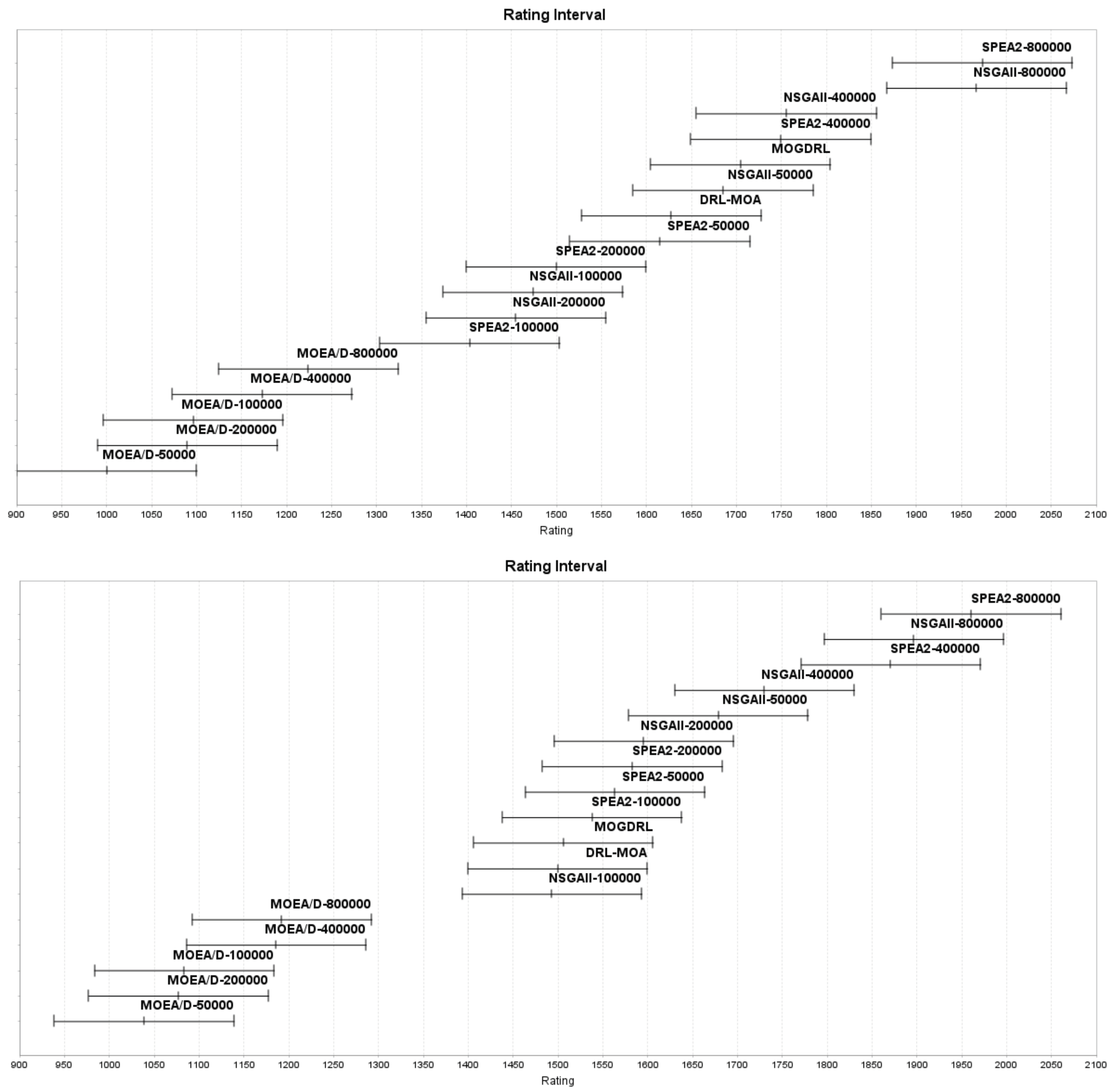
• Fair comparisons: Comparing experiments under the exact same settings is a precondition for all scientific disciplines. Otherwise, the findings may be incorrect and/or misleading, and the derived conclusions may be questionable. TSPs are a popular combinatorial problem that can be solved by algorithms in different categories. In this paper and [7], two kinds of algorithms (i.e., evolutionary algorithms and deep reinforcement learning algorithms) are compared with each other. First, the performance of both kinds of algorithms may be affected greatly by their parameter or hyperparameter settings. The best settings for each algorithm may be investigated first by following [35]. However, the stopping criteria of the two kinds are not comparable. For example, the maximum number of fitness evaluations (maxFEs), maximum number of iterations (maxIter), and max time budget are seen commonly as fixed stopping criteria to terminate evolutionary algorithms. Other criteria, on the other hand, terminate algorithms when the results do not improve any further during the evolutionary process. deep learning algorithms, conversely, use epoch as a fixed stopping criterion. Similarly, some researchers stop deep learning algorithms when loss begins to increase or accuracy begins to decrease. However, the criteria for evolutionary algorithms and those for deep learning algorithms are not always comparable (e.g., maxFEs vs. epoch, or fitness no longer improve vs. accuracy decreases). As observed in Appendices Appendix A.2 and Appendix A.3 in Appendix A, NSGA-II and SPEA2 with 8000 iterations outperformed all the other algorithms in terms of spread and CPF. If there were no such experiments with extra iterations presented, readers would have concluded that MODGRL (or DRL-MOA in some experiments) was the best in terms of all the three quality indicators. With such, max time budget (i.e., maximum CPU time) might be the most objective stopping criteron for comparing algorithms of the same, or even different, categories.
• Performance on Large Scale TSP: MODGRL was trained on a multi-objective TSP with only 40 cities. As is evident from the results obtained from the experiments, it was able to perform well on problems with 100, 150 and 200 cities. Based on this performance, it can be predicted that the MODGRL algorithm can scale very well to even large scale problems with more than 200 cities. Hence, we conducted a number of experiments on 500, 750, and 1000 cities. The experimental results show that MODGRL remained competitive for large scale multi-objective TSPs. Due to the space constraint, the experimental results are not included. Readers may contact the authors for more details.

6. Conclusions

This paper introduces the MODGRL algorithm that incorporates a GPN to provide an added advantage over the other existing deep learning algorithms. The GPN aggregates values from neighboring nodes in order to learn a problem structured in a graph better, such as TSPs. Additionally, a pointer network is capable of handling varying lengths of inputs, which helps overcome the major drawback of having to re-train the algorithm when the problem space changes. As demonstrated by the hypervolume results, MODGRL was only trained on a training set with 40 cities, and it ranked better than DRL-MOA with 100, 150 and 200 cities using the KroAB datasets. The paper also measured the algorithms’ performance using spread and CPF, two popular quality indicators for multi-objective optimization problems. The different ranking results from these three indicators again show the importance of choosing suitable and sufficient quality indicators. In addition to quality indicators, the number of iterations configured for NSGA-II, MODE/D, and SPEA2 also influenced the performance. When the number of iterations was increased to 8000 iterations, NSGA-II and SPEA2 became competitive with MODGRL and DRL-MOA using the KroAB150 and KroAB200 datasets. This extra experiment reminds researchers to avoid the potential pitfall of setting a stopping criterion arbitrarily. Additionally, in order to conduct fair comparisons, it is important to use a stopping criterion that is suitable for all the competing algorithms in different categories (e.g., maximum time budget [14]). Our future direction is to apply MODGRL to other combinatorial optimization problems, such as the job shop scheduling problem (JSSP) [50]. In JSSP, jobs must be processed on machines so that the total completion time is minimal, whilst, in a TSP, the problem is to find the shortest possible route that visits each city exactly once and returns to the city of origin. Both problems, TSP and JSSP, are combinatorial problems which can benefit from pointer network-based reinforcement learning. Our future research aims to investigate what conditions need to be fulfilled to learn graphical structures on small problems that can be applied successfully to larger problems.

References

1. El Naqa, I.; Murphy, M.J. What Is Machine Learning? In Machine Learning in Radiation Oncology: Theory and Applications; El Naqa, I., Li, R., Murphy, M.J., Eds.; Springer International Publishing: Berlin/Heidelberg, Germany, 2015; pp. 3–11. [Google Scholar]
2. Coello Coello, C.A. An Introduction to Evolutionary Algorithms and Their Applications. In Proceedings of the International Symposium and School on Advancex Distributed Systems, Guadalajara, Mexico, 14–18 January 2005; Ramos, F.F., Larios Rosillo, V., Unger, H., Eds.; Springer: Berlin/Heidelberg, Germany, 2005; pp. 425–442. [Google Scholar]
3. Sutton, R.S.; Barto, A.G. Reinforcement Learning: An Introduction; MIT Press: Cambridge, MA, USA, 2014. [Google Scholar]
4. Minsky, M.L. Theory of Neural-Analog Reinforcement Systems and Its Application to the Brain-Model Problem. Ph.D. Thesis, Princeton University, Princeton, NJ, USA, 1954. [Google Scholar]
5. Levin, E.; Pieraccini, R.; Eckert, W. Using Markov decision process for learning dialogue strategies. In Proceedings of the 1998 IEEE International Conference on Acoustics, Speech and Signal Processing, Seattle, WA, USA, 12–15 May 1998; Volume 1, pp. 201–204. [Google Scholar]
6. Miki, S.; Yamamoto, D.; Ebara, H. Applying Deep Learning and Reinforcement Learning to Traveling Salesman Problem. In Proceedings of the 2018 International Conference on Computing, Electronics Communications Engineering, Southend, UK, 16–17 August 2018; pp. 65–70. [Google Scholar]
7. Li, K.; Zhang, T.; Wang, R. Deep Reinforcement Learning for Multiobjective Optimization. IEEE Trans. Cybern. 2020, 51, 3103–3114. [Google Scholar] [CrossRef] [Green Version]
8. Vinyals, O.; Fortunato, M.; Jaitly, N. Pointer Networks. In Proceedings of the Advances in Neural Information Processing Systems, Montreal, QC, Canada, 7–12 December 2015; Cortes, C., Lawrence, N., Lee, D., Sugiyama, M., Garnett, R., Eds.; Curran Associates, Inc.: New York, NY, USA, 2015; Volume 28. [Google Scholar]
9. Nguyen, T.T.; Nguyen, N.D.; Vamplew, P.; Nahavandi, S.; Dazeley, R.; Lim, C.P. A multi-objective deep reinforcement learning framework. Eng. Appl. Artif. Intell. 2020, 96, 103915. [Google Scholar] [CrossRef]
10. Zhou, J.; Cui, G.; Hu, S.; Zhang, Z.; Yang, C.; Liu, Z.; Wang, L.; Li, C.; Sun, M. Graph neural networks: A review of methods and applications. AI Open 2020, 1, 57–81. [Google Scholar] [CrossRef]
11. Ma, Q.; Ge, S.; He, D.; Thaker, D.; Drori, I. Combinatorial Optimization by Graph Pointer Networks and Hierarchical Reinforcement Learning. arXiv 2019, arXiv:1911.04936. [Google Scholar]
12. Ravber, M.; Mernik, M.; Črepinšek, M. The impact of quality indicators on the rating of multi-objective evolutionary algorithms. Appl. Soft Comput. 2017, 55, 265–275. [Google Scholar] [CrossRef]
13. Ravber, M.; Mernik, M.; Črepinšek, M. Ranking multi-objective evolutionary algorithms using a chess rating system with quality indicator ensemble. In Proceedings of the 2017 IEEE Congress on Evolutionary Computation (CEC), Donostia-San Sebastian, Spain, 5–8 June 2017; pp. 1503–1510. [Google Scholar]
14. Ravber, M.; Liu, S.H.; Mernik, M.; Črepinšek, M. Maximum number of generations as a stopping criterion considered harmful. Appl. Soft Comput. 2022, 128, 109478. [Google Scholar] [CrossRef]
15. Deb, K.; Pratap, A.; Agarwal, S.; Meyarivan, T. A fast and elitist multiobjective genetic algorithm: NSGA-II. IEEE Trans. Evol. Comput. 2002, 6, 182–197. [Google Scholar] [CrossRef] [Green Version]
16. Zitzler, E.; Thiele, L. Multiobjective evolutionary algorithms: A comparative case study and the strength Pareto approach. IEEE Trans. Evol. Comput. 1999, 3, 257–271. [Google Scholar] [CrossRef] [Green Version]
17. Santosa, B. Tutorial on Ant Colony Optimization. Institut Teknologi Sepuluh Nopember, ITS. Surabaya. 2012. Available online: https://bsantosa.files.wordpress.com/2015/03/aco-tutorial-english2.pdf (accessed on 22 November 2022).
18. Shamsaldin, A.S.; Rashid, T.A.; Al-Rashid Agha, R.A.; Al-Salihi, N.K.; Mohammadi, M. Donkey and smuggler optimization algorithm: A collaborative working approach to path finding. J. Comput. Des. Eng. 2019, 6, 562–583. [Google Scholar] [CrossRef]
19. Lust, T.; Teghem, J. The Multiobjective Traveling Salesman Problem: A Survey and a New Approach. In Advances in Multi-Objective Nature Inspired Computing; Coello Coello, C.A., Dhaenens, C., Jourdan, L., Eds.; Springer: Berlin/Heidelberg, Germany, 2010; pp. 119–141. [Google Scholar]
20. Cheikhrouhou, O.; Khoufi, I. A Comprehensive Survey on the Multiple Traveling Salesman Problem: Applications, Approaches and Taxonomy. Comput. Sci. Rev. 2021, 40, 100369. [Google Scholar] [CrossRef]
21. Sherstinsky, A. Fundamentals of Recurrent Neural Network (RNN) and Long Short-Term Memory (LSTM) network. Phys. D Nonlinear Phenom. 2020, 404, 132306. [Google Scholar] [CrossRef]
22. Sutskever, I.; Vinyals, O.; Le, Q.V. Sequence to Sequence Learning with Neural Networks. In Proceedings of the 27th International Conference on Neural Information Processing Systems, Montreal, QC, Canada, 8–13 December 2014; Volume 2, pp. 3104–3112. [Google Scholar]
23. Bahdanau, D.; Cho, K.; Bengio, Y. Neural Machine Translation by Jointly Learning to Align and Translate. arXiv 2015. [Google Scholar] [CrossRef]
24. Gambardella, L.M.; Dorigo, M. Ant-Q: A Reinforcement Learning approach to the traveling salesman problem. In Machine Learning Proceedings 1995; Morgan Kaufmann: Burlington, MA, USA, 1995; pp. 252–260. [Google Scholar]
25. Arulkumaran, K.; Deisenroth, M.P.; Brundage, M.; Bharath, A.A. Deep Reinforcement Learning: A Brief Survey. IEEE Signal Process. Mag. 2017, 34, 26–38. [Google Scholar] [CrossRef] [Green Version]
26. Grondman, I.; Busoniu, L.; Lopes, G.A.D.; Babuska, R. A Survey of Actor-Critic Reinforcement Learning: Standard and Natural Policy Gradients. IEEE Trans. Syst. Man, Cybern. Part C (Appl. Rev.) 2012, 42, 1291–1307. [Google Scholar] [CrossRef] [Green Version]
27. Bi, Y.; Meixner, C.C.; Bunyakitanon, M.; Vasilakos, X.; Nejabati, R.; Simeonidou, D. Multi-Objective Deep Reinforcement Learning Assisted Service Function Chains Placement. IEEE Trans. Netw. Serv. Manag. 2021, 18, 4134–4150. [Google Scholar] [CrossRef]
28. Keat, E.Y.; Sharef, N.M.; Yaakob, R.; Kasmiran, K.A.; Marlisah, E.; Mustapha, N.; Zolkepli, M. Multiobjective Deep Reinforcement Learning for Recommendation Systems. IEEE Access 2022, 10, 65011–65027. [Google Scholar] [CrossRef]
29. Zhang, Y.; Wang, J.; Zhang, Z.; Zhou, Y. MODRL/D-EL: Multiobjective Deep Reinforcement Learning with Evolutionary Learning for Multiobjective Optimization. In Proceedings of the 2021 International Joint Conference on Neural Networks (IJCNN), Shenzhen, China, 18–22 July 2021; pp. 1–8. [Google Scholar] [CrossRef]
30. Wu, H.; Wang, J.; Zhang, Z. MODRL/D-AM: Multiobjective Deep Reinforcement Learning Algorithm Using Decomposition and Attention Model for Multiobjective Optimization. arXiv 2020. [Google Scholar] [CrossRef]
31. Wang, H.; Wang, R.; Xu, H.; Kun, Z.; Yi, C.; Niyato, D. Multi-objective Mobile Charging Scheduling on the Internet of Electric Vehicles: A DRL Approach. In Proceedings of the 2021 IEEE Global Communications Conference (GLOBECOM), Rio de Janeiro, Brazil, 4–8 December 2021; pp. 1–6. [Google Scholar] [CrossRef]
32. Hu, C.; Wang, Q.; Gong, W.; Yan, X. Multi-objective deep reinforcement learning for emergency scheduling in a water distribution network. Memetic Comput. 2022, 14, 211–223. [Google Scholar] [CrossRef]
33. Hajiakhondi-Meybodi, Z.; Mohammadi, A.; Abouei, J. Deep Reinforcement Learning for Trustworthy and Time-Varying Connection Scheduling in a Coupled UAV-Based Femtocaching Architecture. IEEE Access 2021, 9, 32263–32281. [Google Scholar] [CrossRef]
34. Ouyang, W.; Wang, Y.; Weng, P.; Han, S. Generalization in Deep RL for TSP Problems via Equivariance and Local Search. arXiv 2022, arXiv:2110.03595. [Google Scholar]
35. Črepinšek, M.; Liu, S.H.; Mernik, M. Replication and Comparison of Computational Experiments in Applied Evolutionary Computing: Common Pitfalls and Guidelines to Avoid Them. Appl. Soft Comput. 2014, 19, 161–170. [Google Scholar] [CrossRef]
36. Ma, M.; Li, H. A hybrid genetic algorithm for solving bi-objective traveling salesman problems. J. Phys. Conf. Ser. 2017, 887, 012065. [Google Scholar] [CrossRef] [Green Version]
37. Li, Y. Deep Reinforcement Learning. arXiv 2018, arXiv:1810.06339. [Google Scholar]
38. Hameed, I. Multi-objective Solution of Traveling Salesman Problem with Time. In Proceedings of the International Conference on Advanced Machine Learning Technologies and Applications 2020, Jaipur, India, 13–15 February 2020; pp. 121–132. [Google Scholar] [CrossRef]
39. Reinelt, G. TSPLIB—A Traveling Salesman Problem Library. ORSA J. Comput. 1991, 3, 376–384. [Google Scholar] [CrossRef]
40. Veček, N.; Mernik, M.; Črepinšek, M. A Chess Rating System for Evolutionary Algorithms: A New Method for the Comparison and Ranking of Evolutionary Algorithms. Inf. Sci. 2014, 277, 656–679. [Google Scholar] [CrossRef]
41. Veček, N.; Črepinšek, M.; Mernik, M. On the influence of the number of algorithms, problems, and independent runs in the comparison of evolutionary algorithms. Appl. Soft Comput. 2017, 54, 23–45. [Google Scholar] [CrossRef]
42. Derrac, J.; García, S.; Molina, D.; Herrera, F. A practical tutorial on the use of nonparametric statistical tests as a methodology for comparing evolutionary and swarm intelligence algorithms. Swarm Evol. Comput. 2011, 1, 3–18. [Google Scholar] [CrossRef]
43. Pernet, C. Null hypothesis significance testing: A short tutorial. F1000Research 2017, 4, 621. [Google Scholar] [CrossRef] [Green Version]
44. While, L.; Hingston, P.; Barone, L.; Huband, S. A Faster Algorithm for Calculating Hypervolume. IEEE Trans. Evol. Comput. 2006, 10, 29–38. [Google Scholar] [CrossRef] [Green Version]
45. Wang, Y.; Wu, L.; Yuan, X. Multi-objective Self-Adaptive Differential Evolution with Elitist Archive and Crowding Entropy-based Diversity Measure. Soft Comput. 2010, 14, 193. [Google Scholar] [CrossRef]
46. Tian, Y.; Cheng, R.; Zhang, X.; Jin, Y. PlatEMO: A MATLAB Platform for Evolutionary Multi-Objective Optimization [Educational Forum]. IEEE Comput. Intell. Mag. 2017, 12, 73–87. [Google Scholar] [CrossRef] [Green Version]
47. Tian, Y.; Cheng, R.; Zhang, X.; Li, M.; Jin, Y. Diversity Assessment of Multi-Objective Evolutionary Algorithms: Performance Metric and Benchmark Problems [Research Frontier]. IEEE Comput. Intell. Mag. 2019, 14, 61–74. [Google Scholar] [CrossRef]
48. Zhou, A.; Jin, Y.; Zhang, Q.; Sendhoff, B.; Tsang, E. Combining Model-based and Genetics-based Offspring Generation for Multi-objective Optimization Using a Convergence Criterion. In Proceedings of the 2006 IEEE International Conference on Evolutionary Computation, Vancouver, BC, Canada, 16–21 July 2006; pp. 892–899. [Google Scholar]
49. Audet, C.; Bigeon, J.; Cartier, D.; Digabel, S.L.; Salomon, L. Performance Indicators in Multiobjective Optimization. Eur. J. Oper. Res. 2021, 292, 397–422. [Google Scholar] [CrossRef]
50. Sršen, S.; Mernik, M. A JSSP solution for production planning optimization combining industrial engineering and evolutionary algorithms. Comput. Sci. Inf. Syst. 2021, 18, 349–378. [Google Scholar] [CrossRef]
Figure 1. Architecture of the GPN showing how each component interacts and integrates together.
Mathematics 11 00437 g001
Figure 2. The Pareto-frontiers of MODGRL, DRL-MOA, NSGA-II, MOEA/D and SPEA2 algorithms on the KroAB 100 dataset.
Mathematics 11 00437 g002
Figure 3. Hypervolume ranking results for 100 cities.
Mathematics 11 00437 g003
Figure 4. Spread ranking results for 100 cities.
Mathematics 11 00437 g004
Figure 5. CPF ranking results for 100 cities.
Mathematics 11 00437 g005