
A New Fuzzy Reinforcement Learning Method for Effective Chemotherapy
 ,
,  ,
,
Abstract
:1. Introduction
2. Preliminaries
3. Caputo–Fabrizio Fractional Model of Cancer Chemotherapy
3.1. Existence and Uniqueness of Solutions of the Cancer Chemotherapy Model
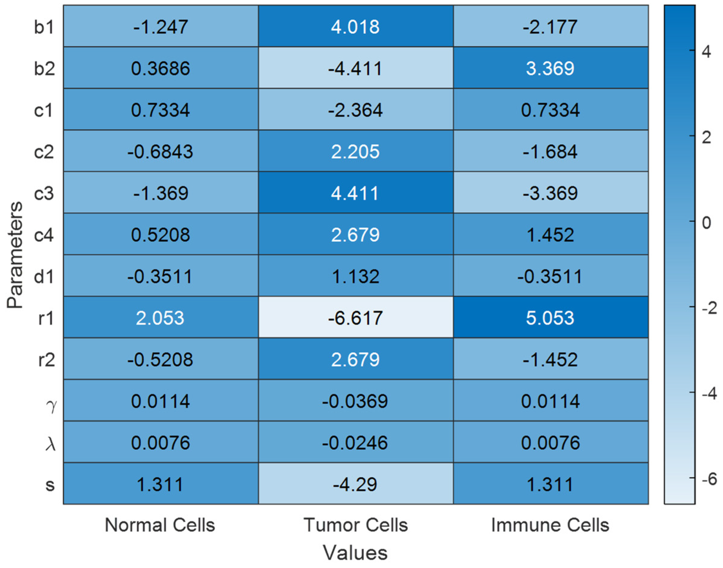
3.2. Sensitivity Analysis
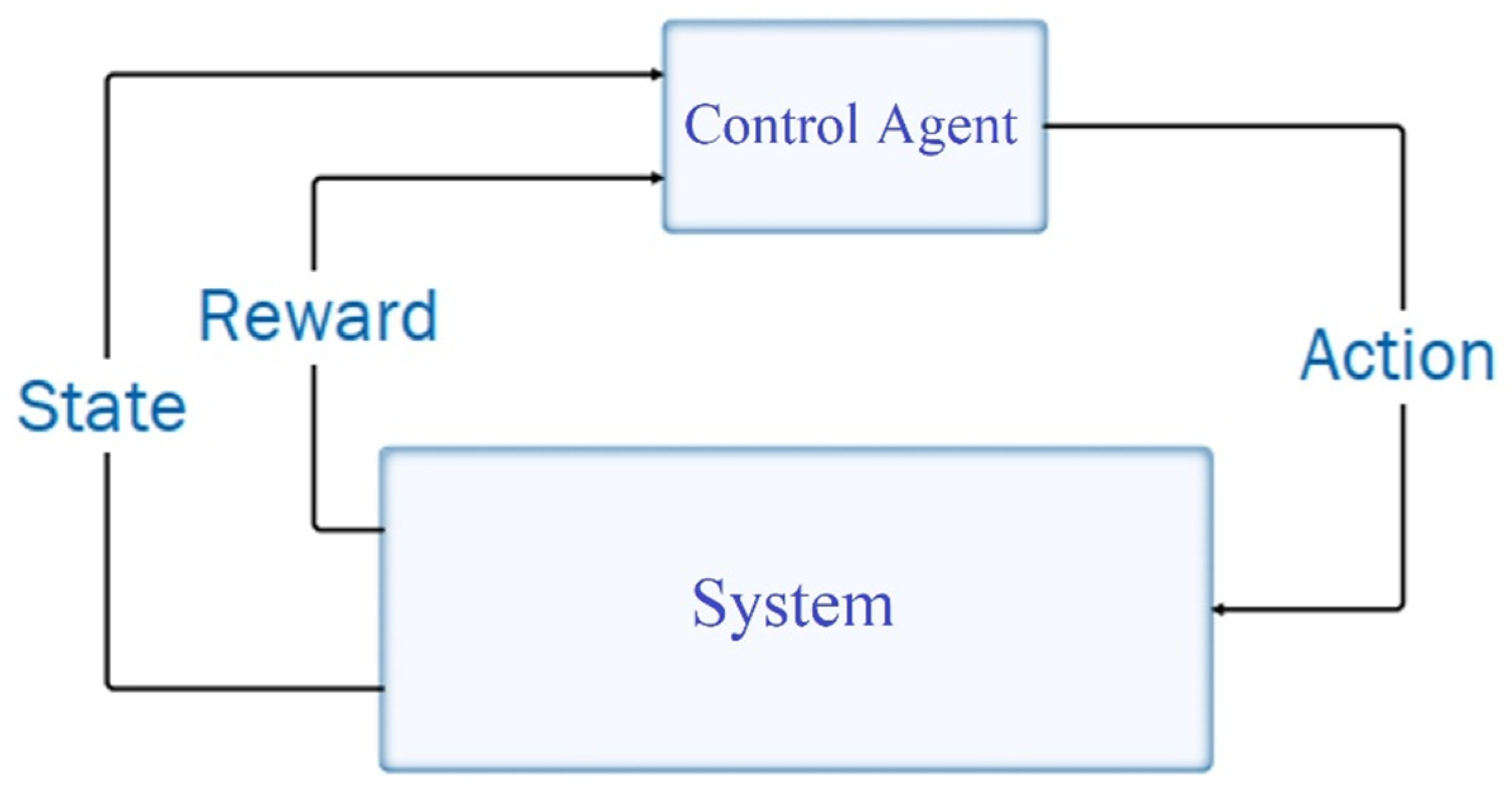
4. Methodology
Fuzzy Controller Based on Expected SARSA Learning (FESL)
| Algorithm 1 Fuzzy Expected SARSA |
| 1: Initialize Q-table 2: Loop {for all of episodes} 3: Initialize state s 4: repeat {for each step in episode} 5: calculate firing strength of each rule (αi) at state s 6: choose action (αi) for each of the rules at state s using policy π 7: calculate action a at state s 8: take action a, observe reward r and next state s′ 9: calculate state value of state s′ 10: update Q-table 11: until s is terminal state 12: end loop |
5. Numerical Simulations
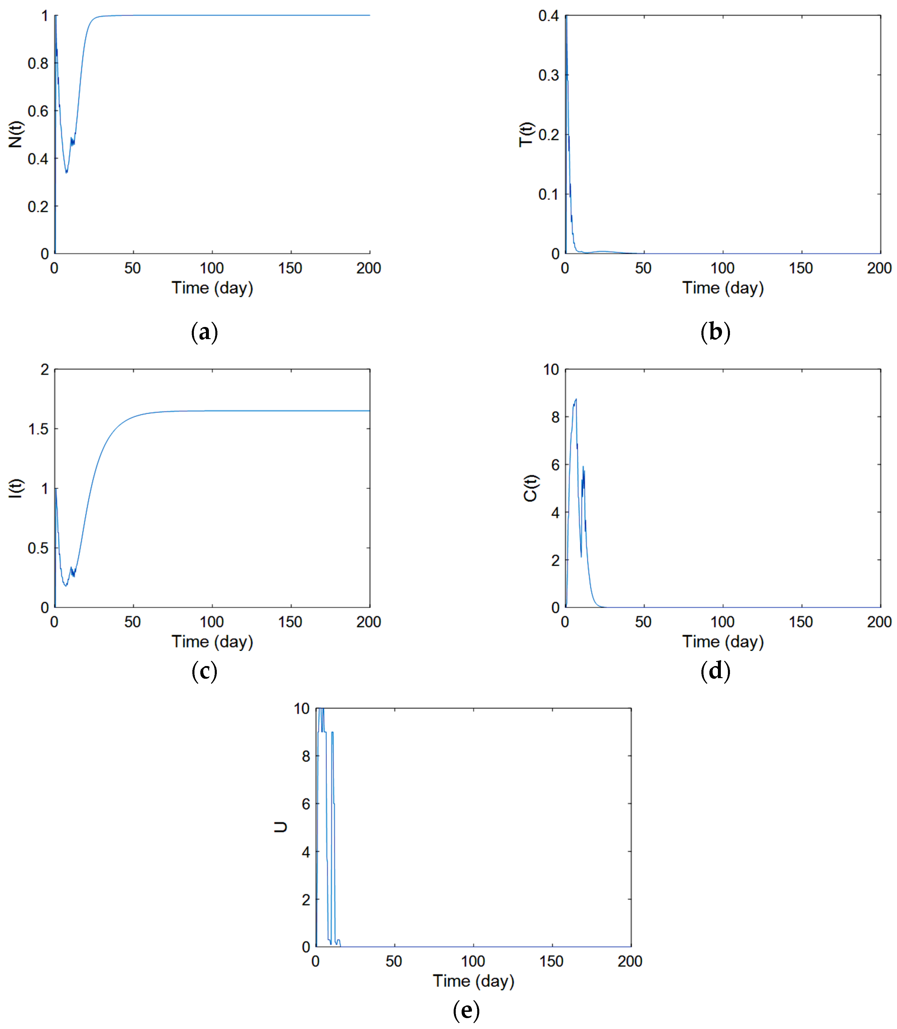
5.1. Scenario A
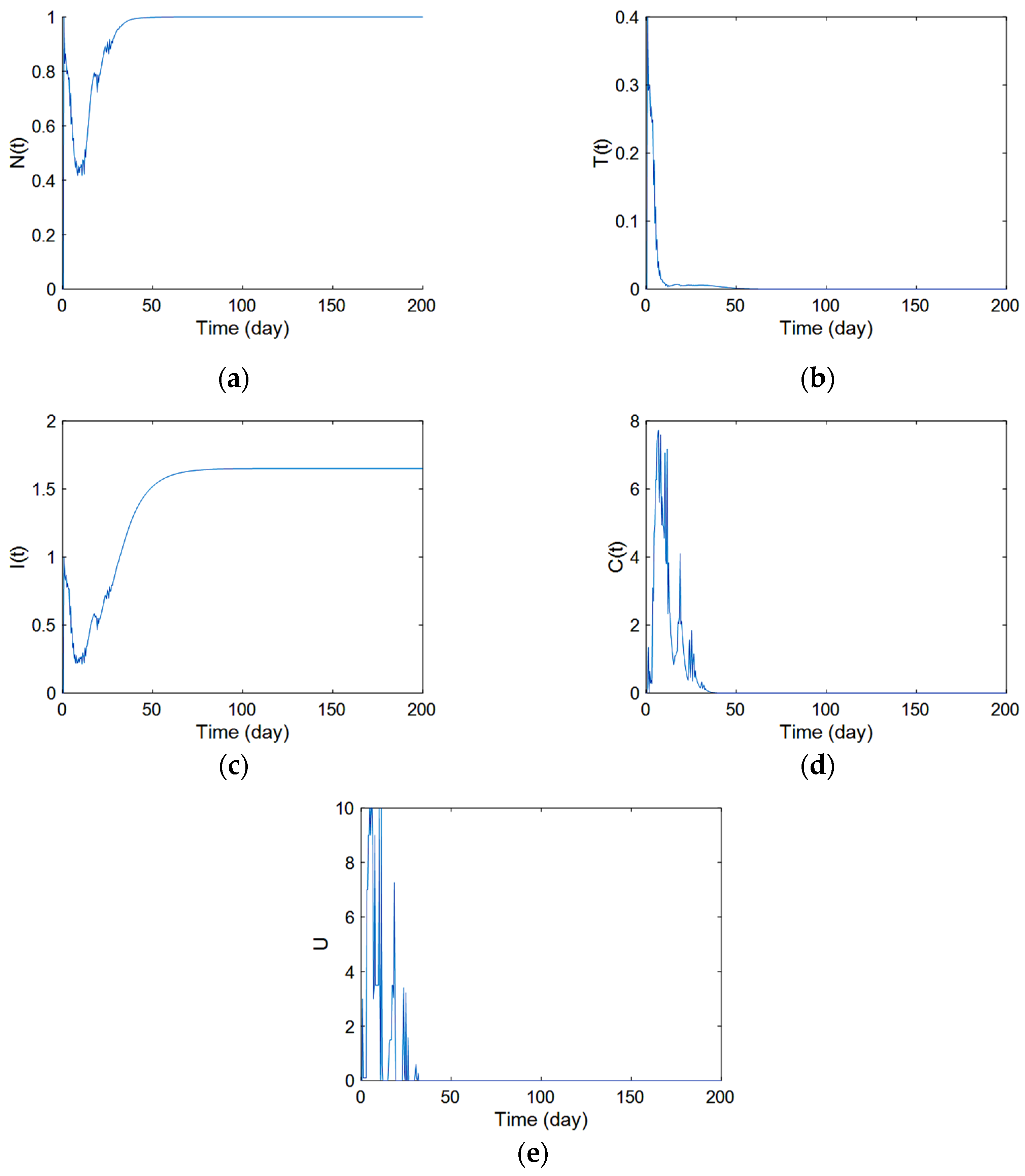
- The effectiveness of the proposed controller in eliminating the tumor cells: The results show that the controller was able to successfully reduce the number of tumor cells to zero, which indicates that the treatment was effective in destroying the cancer cells.
- The temporary decrease in normal cells and immune cells: The chemotherapy used in the treatment caused a temporary decrease in the number of normal cells and immune cells in the body. This is a common side effect of chemotherapy, as the drugs used can also harm healthy cells.
- The recovery of normal cells and immune cells: Despite the initial decrease in normal cells and immune cells, the numbers of these cells eventually increased over time. This suggests that the body was able to recover and rebuild healthy cells after the chemotherapy treatment.
- The importance of monitoring the effects of chemotherapy: The results of the simulation highlight the importance of carefully monitoring the effects of chemotherapy to ensure that it is being administered effectively and safely. This includes monitoring the number of cancer cells, normal cells, and immune cells in the body, as well as the concentration of chemotherapy drugs in the blood.
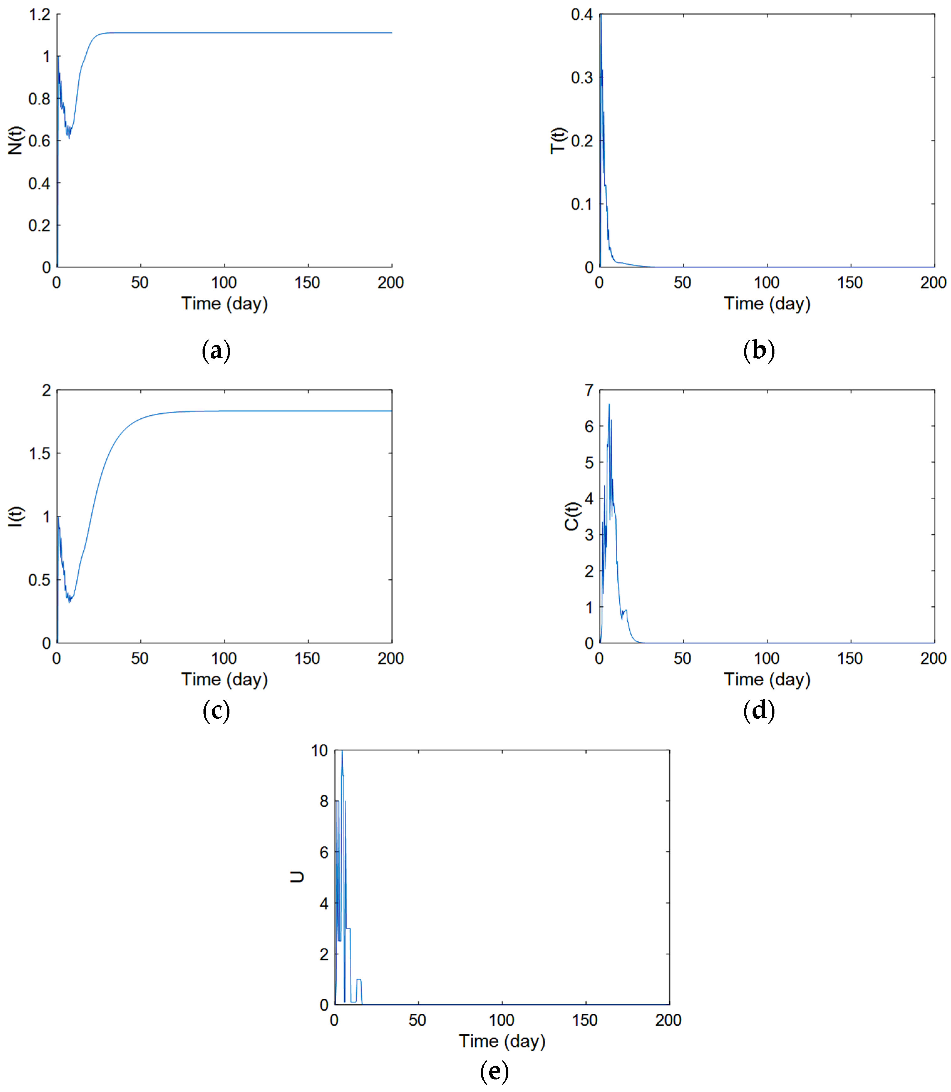
5.2. Scenario B
5.3. Scenario C
6. Conclusions
Author Contributions
Funding
Data Availability Statement
Acknowledgments
Conflicts of Interest
Abbreviations
| FESL | fuzzy controller based on Expected-SARSA learning |
| FRLC | Fuzzy reinforcement learning based controller |
| RL | reinforcement learning |
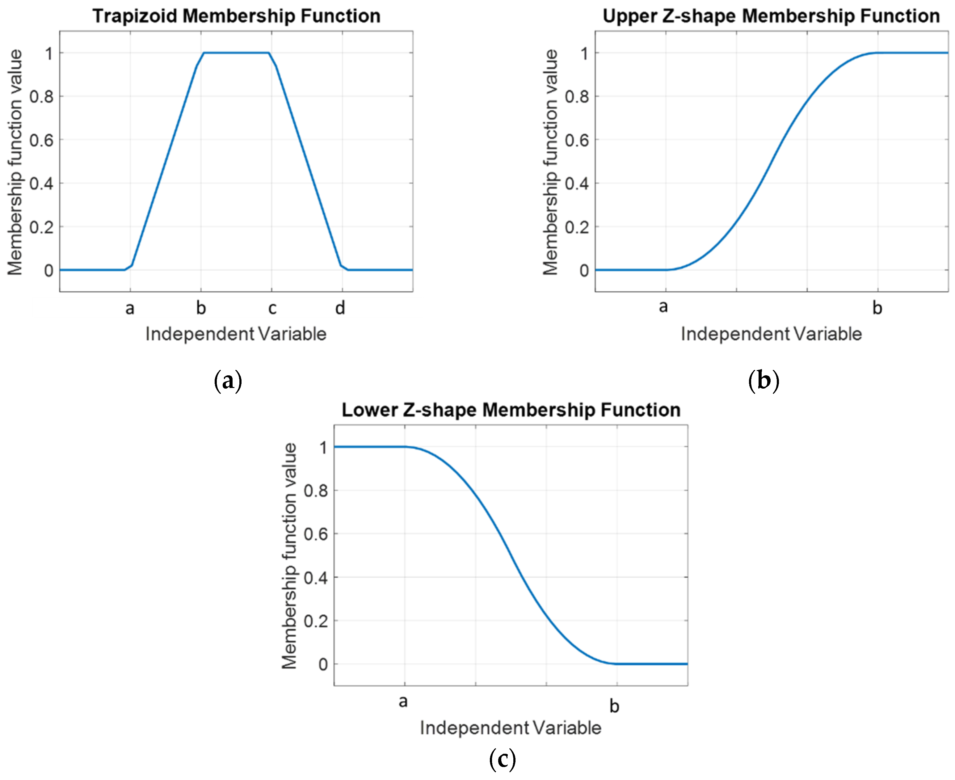
| trapmf | trapezoidal-shape membership function for upper bound |
| SARSA | State-Action-Reward-State-Action |
| zmfl | z-shape membership function for lower bound |
| zmfh | z-shape membership function for upper bound |
References
- Miller, K.D.; Nogueira, L.; Mariotto, A.B.; Rowland, J.H.; Yabroff, K.R.; Alfano, C.M.; Jemal, A.; Kramer, J.L.; Siegel, R.L. Cancer treatment and survivorship statistics, 2019. CA Cancer J. Clin. 2019, 69, 363–385. [Google Scholar] [CrossRef] [PubMed] [Green Version]
- Dos Santos, A.l.F.; De Almeida, D.R.Q.; Terra, L.F.; Baptista, M.c.S.; Labriola, L. Photodynamic therapy in cancer treatment-an update review. J. Cancer Metastasis Treat 2019, 5, 25. [Google Scholar] [CrossRef] [Green Version]
- Thallinger, C.; Füreder, T.; Preusser, M.; Heller, G.; Müllauer, L.; Höller, C.; Prosch, H.; Frank, N.; Swierzewski, R.; Berger, W. Review of cancer treatment with immune checkpoint inhibitors. Wien. Klin. Wochenschr. 2018, 130, 85–91. [Google Scholar] [CrossRef] [Green Version]
- Yagawa, Y.; Tanigawa, K.; Kobayashi, Y.; Yamamoto, M. Cancer immunity and therapy using hyperthermia with immunotherapy, radiotherapy, chemotherapy, and surgery. J. Cancer Metastasis Treat 2017, 3, 218. [Google Scholar] [CrossRef]
- Cui, C.; Yang, J.; Li, X.; Liu, D.; Fu, L.; Wang, X. Functions and mechanisms of circular RNAs in cancer radiotherapy and chemotherapy resistance. Mol. Cancer 2020, 19, 1–16. [Google Scholar] [CrossRef] [Green Version]
- Coates, A.; Abraham, S.; Kaye, S.B.; Sowerbutts, T.; Frewin, C.; Fox, R.M.; Tattersall, M.H.N. On the receiving end—Patient perception of the side-effects of cancer chemotherapy. Eur. J. Cancer Clin. Oncol. 1983, 19, 203–208. [Google Scholar] [CrossRef]
- Toker, D.; Sommer, F.T.; D’Esposito, M. A simple method for detecting chaos in nature. Commun. Biol. 2020, 3, 11. [Google Scholar] [CrossRef] [Green Version]
- Chen, T.; Kirkby, N.F.; Jena, R. Optimal dosing of cancer chemotherapy using model predictive control and moving horizon state/parameter estimation. Comput. Methods Programs Biomed. 2012, 108, 973–983. [Google Scholar] [CrossRef]
- Sbeity, H.; Younes, R. Review of optimization methods for cancer chemotherapy treatment planning. J. Comput. Sci. Syst. Biol. 2015, 8, 74. [Google Scholar] [CrossRef]
- Michor, F. Mathematical models of cancer stem cells. J. Clin. Oncol. 2008, 26, 2854–2861. [Google Scholar] [CrossRef]
- Granata, D.; Lorenzi, L. An Evaluation of Propagation of the HIV-Infected Cells via Optimization Problem. Mathematics 2022, 10, 2021. [Google Scholar] [CrossRef]
- Mokhtare, Z.; Vu, M.T.; Mobayen, S.; Rojsiraphisal, T. An adaptive barrier function terminal sliding mode controller for partial seizure disease based on the Pinsky–Rinzel mathematical model. Mathematics 2022, 10, 2940. [Google Scholar] [CrossRef]
- Jahanshahi, H.; Munoz-Pacheco, J.M.; Bekiros, S.; Alotaibi, N.D. A fractional-order SIRD model with time-dependent memory indexes for encompassing the multi-fractional characteristics of the COVID-19. Chaos Solitons Fractals 2021, 143, 110632. [Google Scholar] [CrossRef] [PubMed]
- Jahanshahi, H. Smooth control of HIV/AIDS infection using a robust adaptive scheme with decoupled sliding mode supervision. Eur. Phys. J. Spec. Top. 2018, 227, 707–718. [Google Scholar] [CrossRef]
- Jahanshahi, H.; Shanazari, K.; Mesrizadeh, M.; Soradi-Zeid, S.; Gómez-Aguilar, J.F. Numerical analysis of Galerkin meshless method for parabolic equations of tumor angiogenesis problem. Eur. Phys. J. Plus 2020, 135, 866. [Google Scholar] [CrossRef]
- Bachmann, J.; Raue, A.; Schilling, M.; Becker, V.; Timmer, J.; Klingmüller, U. Predictive mathematical models of cancer signalling pathways. J. Intern. Med. 2012, 271, 155–165. [Google Scholar] [CrossRef] [PubMed]
- Wilkie, K.P. A review of mathematical models of cancer–immune interactions in the context of tumor dormancy. In Systems Biology of Tumor Dormancy; Springer: Berlin/Heidelberg, Germany, 2013; pp. 201–234. [Google Scholar]
- Brady, R.; Enderling, H. Mathematical models of cancer: When to predict novel therapies, and when not to. Bull. Math. Biol. 2019, 81, 3722–3731. [Google Scholar] [CrossRef] [Green Version]
- Ira, J.I.; Islam, M.S.; Misra, J.C. Mathematical Modelling of the Dynamics of Tumor Growth and its Optimal Control. Preprints 2020, 2020040391. Available online: https://www.preprints.org/manuscript/202004.0391/v2 (accessed on 24 December 2022).
- Eisen, M. Mathematical Models in Cell Biology and Cancer Chemotherapy; Springer Science & Business Media: Berlin/Heidelberg, Germany, 2013; Volume 30. [Google Scholar]
- Schättler, H.; Ledzewicz, U. Optimal Control for Mathematical Models of Cancer Therapies; Springer: Berlin/Heidelberg, Germany, 2015; Volume 42. [Google Scholar]
- Kumar, D.; Singh, J.; Baleanu, D. On the analysis of vibration equation involving a fractional derivative with Mittag-Leffler law. Math. Methods Appl. Sci. 2020, 43, 443–457. [Google Scholar] [CrossRef]
- Soradi-Zeid, S.; Jahanshahi, H.; Yousefpour, A.; Bekiros, S. King algorithm: A novel optimization approach based on variable-order fractional calculus with application in chaotic financial systems. Chaos Solitons Fractals 2020, 132, 109569. [Google Scholar] [CrossRef]
- Kumar, D.; Singh, J.; Al Qurashi, M.; Baleanu, D. A new fractional SIRS-SI malaria disease model with application of vaccines, antimalarial drugs, and spraying. Adv. Differ. Equ. 2019, 2019, 278. [Google Scholar] [CrossRef]
- Srivastava, H.M.; Dubey, V.P.; Kumar, R.; Singh, J.; Kumar, D.; Baleanu, D. An efficient computational approach for a fractional-order biological population model with carrying capacity. Chaos Solitons Fractals 2020, 138, 109880. [Google Scholar] [CrossRef]
- Chen, S.-B.; Jahanshahi, H.; Abba, O.A.; Solís-Pérez, J.E.; Bekiros, S.; Gómez-Aguilar, J.F.; Yousefpour, A.; Chu, Y.-M. The effect of market confidence on a financial system from the perspective of fractional calculus: Numerical investigation and circuit realization. Chaos Solitons Fractals 2020, 140, 110223. [Google Scholar] [CrossRef]
- Chen, S.-B.; Soradi-Zeid, S.; Jahanshahi, H.; Alcaraz, R.; Gómez-Aguilar, J.F.; Bekiros, S.; Chu, Y.-M. Optimal Control of Time-Delay Fractional Equations via a Joint Application of Radial Basis Functions and Collocation Method. Entropy 2020, 22, 1213. [Google Scholar] [CrossRef] [PubMed]
- Singh, J.; Kumar, D.; Baleanu, D. A new analysis of fractional fish farm model associated with Mittag-Leffler-type kernel. Int. J. Biomath. 2020, 13, 2050010. [Google Scholar] [CrossRef]
- Morales-Delgado, V.F.; Gómez-Aguilar, J.F.; Saad, K.; Escobar Jiménez, R.F. Application of the Caputo-Fabrizio and Atangana-Baleanu fractional derivatives to mathematical model of cancer chemotherapy effect. Math. Methods Appl. Sci. 2019, 42, 1167–1193. [Google Scholar] [CrossRef]
- Dokuyucu, M.A.; Celik, E.; Bulut, H.; Baskonus, H.M. Cancer treatment model with the Caputo-Fabrizio fractional derivative. Eur. Phys. J. Plus 2018, 133, 1–6. [Google Scholar] [CrossRef]
- Losada, J.; Nieto, J.J. Properties of a new fractional derivative without singular kernel. Progr. Fract. Differ. Appl. 2015, 1, 87–92. [Google Scholar]
- Caputo, M.; Fabrizio, M. A new definition of fractional derivative without singular kernel. Progr. Fract. Differ. Appl. 2015, 1, 73–85. [Google Scholar]
- Alsaedi, A.; Nieto, J.J.; Venktesh, V. Fractional electrical circuits. Adv. Mech. Eng. 2015, 7, 1687814015618127. [Google Scholar] [CrossRef]
- Singh, J.; Kumar, D.; Baleanu, D. New aspects of fractional Biswas–Milovic model with Mittag-Leffler law. Math. Model. Nat. Phenom. 2019, 14, 303. [Google Scholar] [CrossRef] [Green Version]
- Kumar, D.; Tchier, F.; Singh, J.; Baleanu, D. An efficient computational technique for fractal vehicular traffic flow. Entropy 2018, 20, 259. [Google Scholar] [CrossRef] [PubMed] [Green Version]
- Owolabi, K.M.; Atangana, A. Analysis and application of new fractional Adams–Bashforth scheme with Caputo–Fabrizio derivative. Chaos Solitons Fractals 2017, 105, 111–119. [Google Scholar] [CrossRef]
- Kumar, D.; Singh, J.; Al Qurashi, M.; Baleanu, D. Analysis of logistic equation pertaining to a new fractional derivative with non-singular kernel. Adv. Mech. Eng. 2017, 9, 1687814017690069. [Google Scholar] [CrossRef]
- Tateishi, A.A.; Ribeiro, H.V.; Lenzi, E.K. The role of fractional time-derivative operators on anomalous diffusion. Front. Phys. 2017, 5, 52. [Google Scholar] [CrossRef] [Green Version]
- Atangana, A.; Alkahtani, B. Analysis of the Keller–Segel model with a fractional derivative without singular kernel. Entropy 2015, 17, 4439–4453. [Google Scholar] [CrossRef]
- Diethelm, K. The Analysis of Fractional Differential Equations: An Application-Oriented Exposition Using Differential Operators of Caputo Type; Springer Science & Business Media: Berlin/Heidelberg, Germany, 2010. [Google Scholar]
- Baleanu, D.; Jajarmi, A.; Mohammadi, H.; Rezapour, S. A new study on the mathematical modelling of human liver with Caputo–Fabrizio fractional derivative. Chaos Solitons Fractals 2020, 134, 109705. [Google Scholar] [CrossRef]
- Bushnaq, S.; Khan, S.A.; Shah, K.; Zaman, G. Mathematical analysis of HIV/AIDS infection model with Caputo-Fabrizio fractional derivative. Cogent Math. Stat. 2018, 5, 1432521. [Google Scholar] [CrossRef]
- Ullah, S.; Khan, M.A.; Farooq, M.; Hammouch, Z.; Baleanu, D. A fractional model for the dynamics of tuberculosis infection using Caputo-Fabrizio derivative. Discret. Contin. Dyn. Syst.-S 2020, 13, 975–993. [Google Scholar] [CrossRef] [Green Version]
- Hristov, J. Derivatives with non-singular kernels from the Caputo–Fabrizio definition and beyond: Appraising analysis with emphasis on diffusion models. Front. Fract. Calc. 2017, 1, 270–342. [Google Scholar]
- Liu, P.; Liu, X. Dynamics of a tumor-immune model considering targeted chemotherapy. Chaos Solitons Fractals 2017, 98, 7–13. [Google Scholar] [CrossRef]
- Moradi, H.; Sharifi, M.; Vossoughi, G. Adaptive robust control of cancer chemotherapy in the presence of parametric uncertainties: A comparison between three hypotheses. Comput. Biol. Med. 2015, 56, 145–157. [Google Scholar] [CrossRef]
- De Pillis, L.G.; Radunskaya, A. The dynamics of an optimally controlled tumor model: A case study. Math. Comput. Model. 2003, 37, 1221–1244. [Google Scholar] [CrossRef]
- De Pillis, L.G.; Radunskaya, A. A mathematical tumor model with immune resistance and drug therapy: An optimal control approach. Comput. Math. Methods Med. 2001, 3, 79–100. [Google Scholar] [CrossRef]
- de Pillis, L.G.; Gu, W.; Fister, K.R.; Head, T.A.; Maples, K.; Murugan, A.; Neal, T.; Yoshida, K. Chemotherapy for tumors: An analysis of the dynamics and a study of quadratic and linear optimal controls. Math. Biosci. 2007, 209, 292–315. [Google Scholar] [CrossRef] [PubMed]
- Ghaffari, A.; Naserifar, N. Optimal therapeutic protocols in cancer immunotherapy. Comput. Biol. Med. 2010, 40, 261–270. [Google Scholar] [CrossRef]
- Pang, L.; Zhao, Z.; Song, X. Cost-effectiveness analysis of optimal strategy for tumor treatment. Chaos Solitons Fractals 2016, 87, 293–301. [Google Scholar] [CrossRef]
- Ledzewicz, U.; Schättler, H. Drug resistance in cancer chemotherapy as an optimal control problem. Discret. Contin. Dyn. Syst. -B 2006, 6, 129. [Google Scholar] [CrossRef]
- Arciero, J.C.; Jackson, T.L.; Kirschner, D.E. A mathematical model of tumor-immune evasion and siRNA treatment. Discret. Contin. Dyn. Syst.-B 2004, 4, 39. [Google Scholar]
- Letellier, C.; Sasmal, S.K.; Draghi, C.; Denis, F.; Ghosh, D. A chemotherapy combined with an anti-angiogenic drug applied to a cancer model including angiogenesis. Chaos Solitons Fractals 2017, 99, 297–311. [Google Scholar] [CrossRef]
- Rokhforoz, P.; Jamshidi, A.A.; Sarvestani, N.N. Adaptive robust control of cancer chemotherapy with extended Kalman filter observer. Inform. Med. Unlocked 2017, 8, 1–7. [Google Scholar] [CrossRef]
- Itik, M.; Salamci, M.U.; Banks, S.P. Optimal control of drug therapy in cancer treatment. Nonlinear Anal. Theory Methods Appl. 2009, 71, e1473–e1486. [Google Scholar] [CrossRef]
- Padmanabhan, R.; Meskin, N.; Haddad, W.M. Reinforcement learning-based control of drug dosing for cancer chemotherapy treatment. Math. Biosci. 2017, 293, 11–20. [Google Scholar] [CrossRef] [PubMed]
- Yousefpour, A.; Haji Hosseinloo, A.; Reza Hairi Yazdi, M.; Bahrami, A. Disturbance observer–based terminal sliding mode control for effective performance of a nonlinear vibration energy harvester. J. Intell. Mater. Syst. Struct. 2020, 31, 1495–1510. [Google Scholar] [CrossRef]
- Yousefpour, A.; Yasami, A.; Beigi, A.; Liu, J. On the development of an intelligent controller for neural networks: A type 2 fuzzy and chatter-free approach for variable-order fractional cases. Eur. Phys. J. Spec. Top. 2022, 231, 2045–2057. [Google Scholar] [CrossRef]
- Yousefpour, A.; Jahanshahi, H. Fast disturbance-observer-based robust integral terminal sliding mode control of a hyperchaotic memristor oscillator. Eur. Phys. J. Spec. Top. 2019, 228, 2247–2268. [Google Scholar] [CrossRef]
- Yousefpour, A.; Jahanshahi, H.; Bekiros, S.; Muñoz-Pacheco, J.M. Robust adaptive control of fractional-order memristive neural networks. In Mem-Elements for Neuromorphic Circuits with Artificial Intelligence Applications; Elsevier: Amsterdam, The Netherlands, 2021; pp. 501–515. [Google Scholar]
- Yousefpour, A.; Jahanshahi, H.; Gan, D. Fuzzy integral sliding mode technique for synchronization of memristive neural networks. In Mem-Elements for Neuromorphic Circuits with Artificial Intelligence Applications; Elsevier: Amsterdam, The Netherlands, 2021; pp. 485–500. [Google Scholar]
- Jahanshahi, H.; Sajjadi, S.S.; Bekiros, S.; Aly, A.A. On the development of variable-order fractional hyperchaotic economic system with a nonlinear model predictive controller. Chaos Solitons Fractals 2021, 144, 110698. [Google Scholar] [CrossRef]
- Jahanshahi, H.; Yousefpour, A.; Wei, Z.; Alcaraz, R.; Bekiros, S. A financial hyperchaotic system with coexisting attractors: Dynamic investigation, entropy analysis, control and synchronization. Chaos Solitons Fractals 2019, 126, 66–77. [Google Scholar] [CrossRef]
- Yao, Q.; Jahanshahi, H.; Bekiros, S.; Mihalache, S.F.; Alotaibi, N.D. Gain-Scheduled Sliding-Mode-Type Iterative Learning Control Design for Mechanical Systems. Mathematics 2022, 10, 3005. [Google Scholar] [CrossRef]
- Yao, Q.; Jahanshahi, H.; Batrancea, L.M.; Alotaibi, N.D.; Rus, M.-I. Fixed-Time Output-Constrained Synchronization of Unknown Chaotic Financial Systems Using Neural Learning. Mathematics 2022, 10, 3682. [Google Scholar] [CrossRef]
- Alsaadi, F.E.; Yasami, A.; Alsubaie, H.; Alotaibi, A.; Jahanshahi, H. Control of a Hydraulic Generator Regulating System Using Chebyshev-Neural-Network-Based Non-Singular Fast Terminal Sliding Mode Method. Mathematics 2023, 11, 168. [Google Scholar] [CrossRef]
- Jahanshahi, H.; Yao, Q.; Khan, M.I.; Moroz, I. Unified neural output-constrained control for space manipulator using tan-type barrier Lyapunov function. Adv. Space Res. 2022; in press. [Google Scholar]
- Jahanshahi, H.; Zambrano-Serrano, E.; Bekiros, S.; Wei, Z.; Volos, C.; Castillo, O.; Aly, A.A. On the dynamical investigation and synchronization of variable-order fractional neural networks: The Hopfield-like neural network model. Eur. Phys. J. Spec. Top. 2022, 231, 1757–1769. [Google Scholar] [CrossRef]
- Jahanshahi, H.; Yousefpour, A.; Soradi-Zeid, S.; Castillo, O. A review on design and implementation of type-2 fuzzy controllers. Math. Methods Appl. Sci. 2022. [Google Scholar] [CrossRef]
- Yao, Q.; Jahanshahi, H.; Bekiros, S.; Mihalache, S.F.; Alotaibi, N.D. Indirect neural-enhanced integral sliding mode control for finite-time fault-tolerant attitude tracking of spacecraft. Mathematics 2022, 10, 2467. [Google Scholar] [CrossRef]
- Alsaade, F.W.; Yao, Q.; Bekiros, S.; Al-zahrani, M.S.; Alzahrani, A.S.; Jahanshahi, H. Chaotic attitude synchronization and anti-synchronization of master-slave satellites using a robust fixed-time adaptive controller. Chaos Solitons Fractals 2022, 165, 112883. [Google Scholar] [CrossRef]
- Yao, Q.; Jahanshahi, H.; Moroz, I.; Bekiros, S.; Alassafi, M.O. Indirect neural-based finite-time integral sliding mode control for trajectory tracking guidance of Mars entry vehicle. Adv. Space Res. 2022; in press. [Google Scholar]
- Chen, X. Research on application of artificial intelligence model in automobile machinery control system. Int. J. Heavy Veh. Syst. 2020, 27, 83–96. [Google Scholar] [CrossRef]
- Das, P.; Chanda, S.; De, A. Artificial Intelligence-Based Economic Control of Micro-grids: A Review of Application of IoT. In Computational Advancement in Communication Circuits and Systems; Springer: Berlin/Heidelberg, Germany, 2020; pp. 145–155. [Google Scholar]
- Hamet, P.; Tremblay, J. Artificial intelligence in medicine. Metabolism 2017, 69, S36–S40. [Google Scholar] [CrossRef]
- Lim, C.W.; Zhang, G.; Reddy, J.N. A higher-order nonlocal elasticity and strain gradient theory and its applications in wave propagation. J. Mech. Phys. Solids 2015, 78, 298–313. [Google Scholar] [CrossRef]
- Mao, Y.; Wang, J.; Jia, P.; Li, S.; Qiu, Z.; Zhang, L.; Han, Z. A reinforcement learning based dynamic walking control. In Proceedings of the 2007 IEEE International Conference on Robotics and Automation, Rome, Italy, 10–14 April 2007; pp. 3609–3614. [Google Scholar]
- Qiao, J.; Hou, Z.; Ruan, X. Application of reinforcement learning based on neural network to dynamic obstacle avoidance. In Proceedings of the 2008 International Conference on Information and Automation, Changsha, China, 20–23 June 2008; pp. 784–788. [Google Scholar]
- Wei, C.; Zhang, Z.; Qiao, W.; Qu, L. Reinforcement-learning-based intelligent maximum power point tracking control for wind energy conversion systems. IEEE Trans. Ind. Electron. 2015, 62, 6360–6370. [Google Scholar] [CrossRef]
- Sabatier, J.; Farges, C.; Merveillaut, M.; Feneteau, L. On observability and pseudo state estimation of fractional order systems. Eur. J. Control 2012, 18, 260–271. [Google Scholar] [CrossRef]
- Wang, S.; He, S.; Yousefpour, A.; Jahanshahi, H.; Repnik, R.; Perc, M. Chaos and complexity in a fractional-order financial system with time delays. Chaos Solitons Fractals 2020, 131, 109521. [Google Scholar] [CrossRef]
- Kilbas, A.A.; Srivastava, H.M.; Trujillo, J.J. Theory and Applications of Fractional Differential Equations; Elsevier: Amsterdam, The Netherlands, 2006; Volume 204. [Google Scholar]
- Moore, B.L.; Pyeatt, L.D.; Kulkarni, V.; Panousis, P.; Padrez, K.; Doufas, A.G. Reinforcement learning for closed-loop propofol anesthesia: A study in human volunteers. J. Mach. Learn. Res. 2014, 15, 655–696. [Google Scholar]
- Martín-Guerrero, J.D.; Gomez, F.; Soria-Olivas, E.; Schmidhuber, J.; Climente-Martí, M.; Jiménez-Torres, N.V. A reinforcement learning approach for individualizing erythropoietin dosages in hemodialysis patients. Expert Syst. Appl. 2009, 36, 9737–9742. [Google Scholar] [CrossRef]
- Padmanabhan, R.; Meskin, N.; Haddad, W.M. Closed-loop control of anesthesia and mean arterial pressure using reinforcement learning. Biomed. Signal Process. Control 2015, 22, 54–64. [Google Scholar] [CrossRef]
- Batmani, Y.; Khaloozadeh, H. Optimal chemotherapy in cancer treatment: State dependent Riccati equation control and extended Kalman filter. Optim. Control Appl. Methods 2013, 34, 562–577. [Google Scholar] [CrossRef]
- Hunter, J.K.; Nachtergaele, B. Applied Analysis; World Scientific Publishing Company, Toh Tuck Link: Singapore, 2001. [Google Scholar]
- Kreyszig, E. Introductory Functional Analysis with Applications; Wiley: New York, NY, USA, 1978; Volume 1. [Google Scholar]
- Baird, L. Residual algorithms: Reinforcement learning with function approximation. In Machine Learning Proceedings 1995; Elsevier: Amsterdam, The Netherlands, 1995; pp. 30–37. [Google Scholar]
- Gordon, G.J. Stable function approximation in dynamic programming. In Machine Learning Proceedings 1995; Elsevier: Amsterdam, The Netherlands, 1995; pp. 261–268. [Google Scholar]
- Boyan, J.A.; Moore, A.W. Generalization in reinforcement learning: Safely approximating the value function. In Advances in Neural Information Processing Systems; MIT Press: Cambridge, MA, USA, 1995; pp. 369–376. [Google Scholar]
- Kuznetsov, V.A.; Makalkin, I.A.; Taylor, M.A.; Perelson, A.S. Nonlinear dynamics of immunogenic tumors: Parameter estimation and global bifurcation analysis. Bull. Math. Biol. 1994, 56, 295–321. [Google Scholar] [CrossRef]


| Parameter | Description (Unit) | Value |
|---|---|---|
| Fractional immune cell kill rate (mg−1 lday−1) | 0.2 | |
| Fractional tumor cell kill rate (mg−1 lday−1) | 0.3 | |
| Fractional normal cell kill rate (mg−1 lday−1) | 0.1 | |
| Reciprocal carrying capacity of tumor cells (cell−1) | 1 | |
| Reciprocal carrying capacity of normal cells (cell−1) | 1 | |
| Immune cell competition term (competition between immune and tumor cells) (cell−1 day−1) | 1 | |
| Tumor cell competition term (competition between immune and tumor cells) (cell−1 day−1) | 0.5 | |
| Tumor cell competition term (competition between normal and tumor cells) (cell−1 day−1) | 1 | |
| Normal cell competition term (competition between normal and tumor cells) (cell−1 day−1) | 1 | |
| Immune cell death rate (day−1) | 0.2 | |
| Decay rate of injected drug (day−1) | 1 | |
| Per unit growth rate of tumor cells (day−1) | 1.5 | |
| Per unit growth rate of normal cells (day−1) | 1 | |
| Immune cell influx rate (cell day−1) | 0.33 | |
| Immune threshold rate (cell) | 0.3 | |
| Immune response rate (day−1) | 0.01 |
| # | Type | [a, b, c, d] | # | Type | [a, b, c, d] |
|---|---|---|---|---|---|
| 1 | zmfl | [0.0055, 0.0068, ~, ~] | 11 | trapmf | [0.3495, 0.3505, 0.3995, 0.4005] |
| 2 | trapmf | [0.0058, 0.0068, 0.0120, 0.0130] | 12 | trapmf | [0.3995, 0.4005, 0.4495, 0.4505] |
| 3 | trapmf | [0.0120, 0.0130, 0.0245, 0.0255] | 13 | trapmf | [0.4495, 0.4505, 0.4995, 0.5005] |
| 4 | trapmf | [0.0245, 0.0255, 0.0395, 0.0405] | 14 | trapmf | [0.4995, 0.5005, 0.5495, 0.5505] |
| 5 | trapmf | [0.0395, 0.0405, 0.0495, 0.0505] | 15 | trapmf | [0.5495, 0.5505, 0.5995, 0.6005] |
| 6 | trapmf | [0.0495, 0.0505, 0.0995, 0.1005] | 16 | trapmf | [0.5995, 0.6005, 0.6495, 0.6505] |
| 7 | trapmf | [0.0995, 0.1005, 0.1995, 0.2005] | 17 | trapmf | [0.6495, 0.6505, 0.6995, 0.7005] |
| 8 | trapmf | [0.1995, 0.2005, 0.2495, 0.2505] | 18 | trapmf | [0.6995, 0.7005, 0.7995, 0.8005] |
| 9 | trapmf | [0.2495, 0.2505, 0.2995, 0.3005] | 19 | trapmf | [0.7995, 0.8005, 0.8995, 0.9005] |
| 10 | trapmf | [0.2995, 0.3005, 0.3495, 0.3505] | 20 | zmfh | [0.8995, 0.9005, ~, ~] |
| Young Patients | Old Patients | |||||
|---|---|---|---|---|---|---|
| FESL | 1.9633 | 0.0011 | 130.1827 | 3.0863 | 0.0011 | 123.0201 |
| Q-Learning | 3.0206 | 0.0079 | 131.7332 | 4.1083 | 0.0066 | 137.0524 |
Disclaimer/Publisher’s Note: The statements, opinions and data contained in all publications are solely those of the individual author(s) and contributor(s) and not of MDPI and/or the editor(s). MDPI and/or the editor(s) disclaim responsibility for any injury to people or property resulting from any ideas, methods, instructions or products referred to in the content. |
© 2023 by the authors. Licensee MDPI, Basel, Switzerland. This article is an open access article distributed under the terms and conditions of the Creative Commons Attribution (CC BY) license (https://creativecommons.org/licenses/by/4.0/).
Share and Cite
Alsaadi, F.E.; Yasami, A.; Volos, C.; Bekiros, S.; Jahanshahi, H. A New Fuzzy Reinforcement Learning Method for Effective Chemotherapy. Mathematics 2023, 11, 477. https://doi.org/10.3390/math11020477
Alsaadi FE, Yasami A, Volos C, Bekiros S, Jahanshahi H. A New Fuzzy Reinforcement Learning Method for Effective Chemotherapy. Mathematics. 2023; 11(2):477. https://doi.org/10.3390/math11020477
Chicago/Turabian StyleAlsaadi, Fawaz E., Amirreza Yasami, Christos Volos, Stelios Bekiros, and Hadi Jahanshahi. 2023. "A New Fuzzy Reinforcement Learning Method for Effective Chemotherapy" Mathematics 11, no. 2: 477. https://doi.org/10.3390/math11020477