Article

What Is the Best Way to Optimally Parameterize the MPC Cost Function for Vehicle Guidance?

1
Institute of Automatic Control (IRT), RWTH Aachen University, D-52074 Aachen, Germany
2
Department Automated Driving Functions, IAV GmbH, D-09120 Chemnitz, Germany
3
Faculty of Automotive Engineering, Zwickau University of Applied Sciences, D-08056 Zwickau, Germany
4
Faculty of Engineering, HTWK Leipzig University of Applied Sciences, D-04277 Leipzig, Germany
*
Author to whom correspondence should be addressed.
Mathematics 2023, 11(2), 465; https://doi.org/10.3390/math11020465
Submission received: 10 December 2022 / Revised: 10 January 2023 / Accepted: 12 January 2023 / Published: 15 January 2023

Abstract

:
Model predictive control (MPC) is a promising approach to the lateral and longitudinal control of autonomous vehicles. However, the parameterization of the MPC with respect to high-level requirements such as passenger comfort, as well as lateral and longitudinal tracking, is challenging. Numerous tuning parameters and conflicting requirements need to be considered. In this paper, we formulate the MPC tuning task as a multi-objective optimization problem. Its solution is demanding for two reasons: First, MPC-parameterizations are evaluated in a computationally expensive simulation environment. As a result, the optimization algorithm needs to be as sample-efficient as possible. Second, for some poor parameterizations, the simulation cannot be completed; therefore, useful objective function values are not available (for instance, learning with crash constraints). In this work, we compare the sample efficiency of multi-objective particle swarm optimization (MOPSO), a genetic algorithm (NSGA-II), and multiple versions of Bayesian optimization (BO). We extend BO by introducing an adaptive batch size to limit the computational overhead. In addition, we devise a method to deal with crash constraints. The results show that BO works best for a small budget, NSGA-II is best for medium budgets, and none of the evaluated optimizers are superior to random search for large budgets. Both proposed BO extensions are, therefore, shown to be beneficial.

1. Introduction

In recent decades, automated and autonomous driving has become an important topic in automotive technology. Particularly good results have been obtained in limited operational design domains, such as highway driving and park scenarios. In this context, numerous approaches to longitudinal and lateral control have emerged for driver-assistance systems and automated driving functions (e.g., [1,2,3,4,5,6]).
As it became desirable to extend automation and assistance functions into unstructured situations and more complex traffic scenarios, optimization-based approaches, especially model predictive control (MPC), were established for vehicle guidance [7]. MPC allows for us to define the resulting behavior of the vehicles using a cost function and a prediction horizon. However, the optimization-based methods are accompanied by a high numerical effort, especially for the nonlinear vehicle dynamics considered here. Therefore, efficient methods for the treatment of such problems have been developed [8]. However, the manual tuning of the MPC cost function is challenging for complex, high-level criteria such as comfort.
As an alternative, numerous optimization approaches have been presented for single-objective MPC tuning (e.g., [9,10,11,12,13,14]). This paper provides an example of how to formulate the tuning task as a multi-objective black-box optimization problem. Multi-objective optimization allows for us to simultaneously address conflicting objectives such as comfort and tracking accuracy. In order to assess an MPC parameterization on a meaningful driving cycle, an expensive-to-evaluate, closed-loop simulation of the vehicle in its environment is used. As an additional challenge, objective function values are unavailable for some parameterizations due to failing simulations (crash constraints [15]). As the simulation environment is a black box to the optimizer, objectives, tuning parameters, and models can easily be exchanged with the presented approach.
For single-objective optimization and limited budgets, Bayesian optimization (BO) has been shown to require less expensive simulations (i.e., it has a better sample efficiency) than population-based metaheuristics for multiple control-related applications [16]. Therefore, multi-objective BO (MOBO) is a promising candidate for the multi-objective tuning problem. MOBO has seen a fair amount of applications in the control and robotics community (e.g., [17,18,19,20]). In our previous work [21], we also introduced MOBO to MPC parameter tuning.
However, the choice of the acquisition function heavily influences the sample efficiency and computational overhead of MOBO. Most of the previous work on MOBO for controller tuning [17,18,19] used the so-called expected improvement of hypervolume (EIHV) acquisition function [22]. However, the expected improvement-matrix (EIM) criterion [23], as well as Thompson sampling efficient multi-objective optimization (TSEMO) [24], were shown to have a similar sample efficiency, with less computational overhead than EIHV [23,24]. In our previous work with EIM [21], the computational overhead quickly grew with increasing objective function evaluations. In contrast to EIM and EIHV, TSEMO comes with a straightforward heuristic for batch evaluations [24] and is, therefore, expected to scale better.
Previous works on MOBO for controller tuning did not study which version of BO is more sample-efficient than metaheuristics. Therefore, our work compares the sample efficiency and the computational overhead of five different MOBO versions and two metaheuristics, Multiple Objective Particle Swarm Optimization (MOPSO) and Non-dominated Sorting Genetic Algorithm II (NSGA-II), on the vehicle guidance task. Additional benchmarks are random search and grid search. Furthermore, we extend TSEMO to address crashing simulations and adaptive batch sizes.
The paper is structured as follows. After the introduction, we provide a more detailed definition of the application-independent multi-objective MPC tuning problem in Section 2. Afterwards, Section 3 describes and discusses the exemplary MPC tuning framework used here. The investigated algorithms are presented in Section 4, followed by benchmark results in Section 5. The results also highlight the practical applications of the presented approach. After that, the paper concludes with a summary of the results (Section 6).

2. Problem Statement

We formulate the MPC tuning problem as a deterministic multi-objective optimization problem
min θ R N J ( θ ) = J 1 ( θ ) , J 2 ( θ ) , , J M ( θ ) s . t . θ min θ θ max l ( θ ) = 1 .
with M 2 individual objective functions and a vector of N decision variables θ = θ 1 , θ 2 , , θ N . The individual objective functions J i ( θ ) : R N R , i { 1 , 2 , M } describe several aims or targets of the overall control behavior, and the decision variables θ i are specific MPC parameters. The vectors of the upper and lower bounds of the decision variables are denoted with θ max and θ min , respectively. The set
Θ f = θ R N θ min θ θ max ; l ( θ ) = 1
is the feasible set of decision vectors representing the feasible domain in the decision space.
In addition to the objective function values, decision variables are also crucial to the valuation of an MPC parameterization, and whether or not it causes the system to crash. To formalize this criterion, we defined the function l ( θ ) , which returns 1 in the positive case and 0 in the crash case. The function is part of the equality constraint of the optimization problem (1), termed the crash constraint, and thus has a direct influence on the feasible domain Θ f . In case of a system crash l ( θ ) = 0 , objective function values are unavailable. Note that, in general, there is no analytical description of the function l ( θ ) for the MPC tuning problem. This setting is also known as learning with crash constraint [15].
In multi-objective optimization, there is usually no feasible solution that simultaneously minimizes all objective functions. Generally, if one objective is improved, other objectives are degraded. Thus, the superiority of one solution over other solutions cannot be determined by comparing their objective function values, as in the single-objective optimization case. Therefore, the focus is on Pareto optimal solutions. Here, the goodness of a solution is determined by its dominance. A feasible solution θ a Θ f is said to dominate another solution θ b Θ f , denoted with θ a θ b , if, and only if,
i { 1 , 2 , , M } : J i ( θ a ) J i ( θ b ) and j { 1 , 2 , , M } : J j ( θ a ) < J j ( θ b ) .
A solution θ * Θ f is said to be Pareto-optimal if no other solution exist in the feasible domain that dominates it. The set of all Pareto optimal solutions in the feasible domain, denoted Θ po , is called the Pareto optimal solution set. It is defined as:
Θ po = θ * Θ f ¬ θ Θ f : θ θ * .
The set of objective function vectors corresponding to the Pareto optimal solution set Θ po is the Pareto front. It is defined as:
J po = J ( θ * ) = J 1 ( θ * ) , , J M ( θ * ) θ * Θ po .
This set is also known as the Pareto optimal frontier or Pareto equilibrium surface.
The result of solving the multi-objective optimization problem (1) is the Pareto optimal solution set J po , which is a set of solutions that defines the best tradeoff between competing objectives. Knowledge of the Pareto optimal solution set and its corresponding Pareto front J po allows for specific MPC parameterizations to be set for specific use cases. Therefore, it is necessary to decide which objectives are of particular importance for a specific use-case.
In general, solving such a multi-objective optimization problem is very time-consuming and provides only an approximation of the Pareto front. Therefore, it is important to use a suitable approach for this purpose, which provides a good approximation of the Pareto front with low computational effort. The comparison of different methods for MPC tuning is the main focus of this paper.
In this paper, one MPC parameterization θ is evaluated using a closed-loop simulation of the vehicle in its environment. This poses two challenges for the multi-objective optimization algorithm. First, an analytical description of the objective function is not available. Instead, the optimizer can only query the simulation environment with the parameters and record the responses. This setting is known as black-box optimization. Second, each simulation takes a considerable amount of time. Therefore the sample efficiency, i.e., an optimizer’s ability to approximately solve (1) with as few objective function evaluations as possible, is of major importance.

3. Simulation-Based MPC Tuning for Vehicle Guidance

This section introduces the paper’s specific MPC tuning case study as a special case of the problem formulated in Section 2. The task is to optimize the parameterization of a model predictive controller for the longitudinal and lateral guidance of vehicles using a simulation. The optimization procedure is repeated several times with each optimization algorithm in Section 5 to generate statistically significant results. In this context, the test case is designed so that the optimization time does not prohibitively increase. However, the problem formulation in Section 2 encompasses a wide variety of alternative use-cases, and the algorithms presented in Section 4 are not in any way restricted to the following exemplary test case. Due to the black-box nature of the optimization algorithms, any kind of simulation environment, vehicle model, objective functions, tuning parameter, and parameter bounds can be optimized in principle. The practical viability of the optimizers in more complex settings may be addressed in future work.

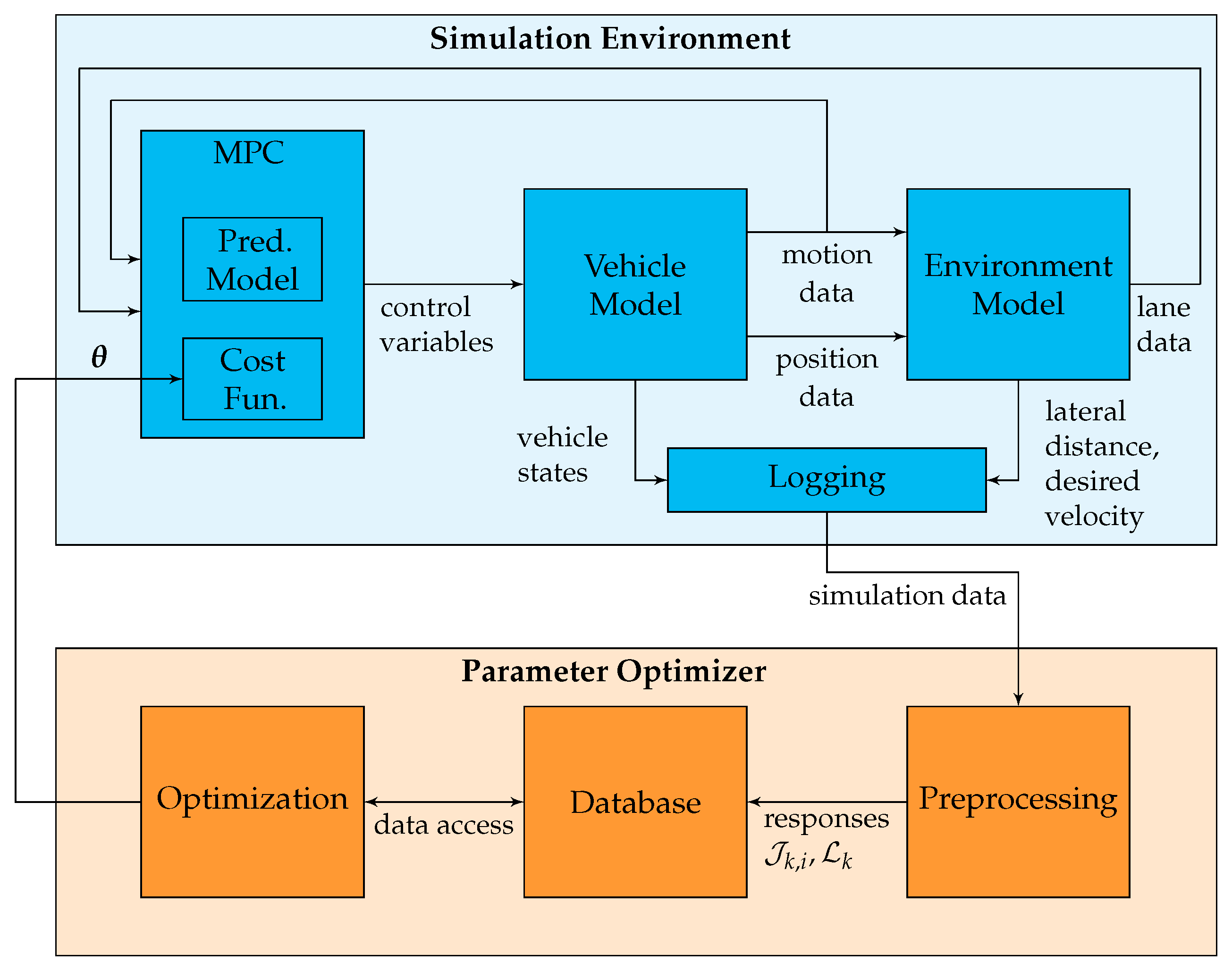
3.1. Controller Tuning Framework

To find the optimal MPC parameterizations, we propose a controller tuning framework, as shown in Figure 1, which consists of two main parts: the parameter optimizer and the simulation environment. Note that we used the framework for MPC parameter tuning, but it can easily be adapted for any other type of controller parameter tuning.
The parameter optimizer handles the complete optimization process. This includes preprocessing, database and optimization, which receive, store, and pre-process the simulation data (i.e., calculating the objective function values from the time domain data), invoking the optimization algorithm with the stored data and querying the simulation environment with a specific parameter vector θ . How often and in which order these actions are performed depends on the multi-objective optimization algorithm that is used. For optimization, we considered different multi-objective Bayesian optimizations (MOBO) and two metaheuristics, Multiple Objective Particle Swarm Optimization (MOPSO) and Non-dominated Sorting Genetic Algorithm II (NSGA-II); see Section 4 for details.
To evaluate the control performance of the MPC for a given parameter vector θ , the simulation environment was utilized. For this purpose, the MPC was simulated in closed-loop with a nonlinear plant. The plant consisted of two main parts: a vehicle model and an environment model. The vehicle model was a combination of simple drive train model, a steering actuator model and a bicycle model, as described in [25]. This determined the lateral and longitudinal behavior of the ego vehicle, depending on the control inputs and the feedback from the environment model. Its outputs were the states of the ego vehicle, such as its velocity, position, or orientation. Based on the states of the ego vehicle, the environment model provides input data for the MPC controller. In our case, this was lane data, obtained using idealized lane detection for a predefined virtual road with two lanes. Furthermore, the simulation environment had appropriate interfaces with the parameter optimizer to receive the input data and provide the simulation data.
The simulation environment was implemented using MATLAB/Simulink. As mentioned above, the simulation duration has a crucial impact on the overall tuning duration. Therefore, we minimized the simulation duration by exporting the Simulink model as an executable that runs fast, standalone simulations. This was achieved using the rapid simulation (RSim) feature of Simulink and allowed for us to repeat simulations with varying inputs without rebuilding the model.

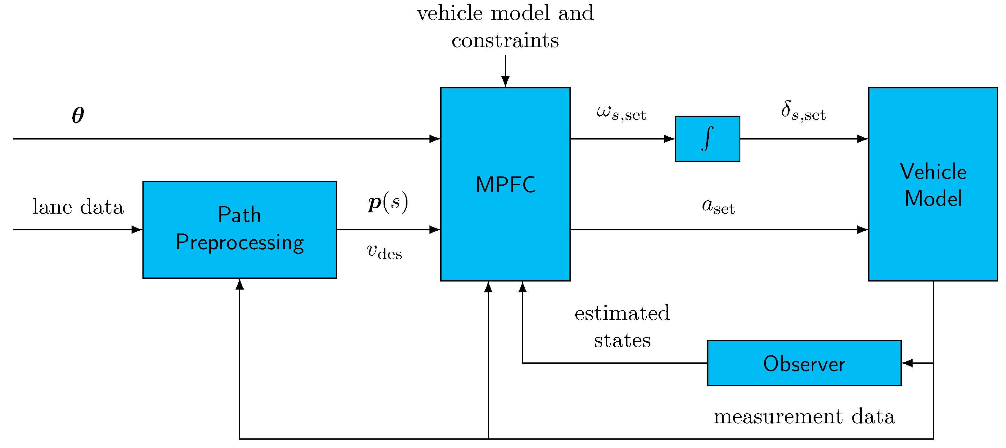
3.2. MPC for Vehicle Guidance

The subject of our studies is the parameter tuning of the MPC realization presented in [25]. This MPC realization is designed for longitudinal and lateral vehicle control and is based on the so-called model predictive path-following control (MPFC) approach, a nonlinear MPC approach presented in [26]. We will provide a brief overview of this MPC realization in the following. For a more comprehensive description, refer to [25].
The main idea of this MPC realization is that the system, i.e., the ego vehicle, follows a given geometric reference path (e.g., the coordinates of the driving lane center). The reference path is given as a parametrized regular curve p : s [ 0 , s max ] R 3 , where s R is the so-called path parameter. This reference path is defined as
p ( s ) = x des ( s ) y des ( s ) ψ des ( s ) ,
where x des ( s ) and y des ( s ) are cubic splines and ψ des ( s ) is calculated with
ψ des ( s ) = arctan y des s x des s 1 .
Note that the splines x des and y des only describe the path for a limited horizon and, therefore, are continuously updated online based on sensor data.
The behavior of the ego vehicle is modeled as a continuous-time nonlinear system, as described in [25]. The control input u = [ a set , ω set ] consists of the target acceleration a set and the steering wheel target angular velocity ω s , set . Furthermore, the output vector y = [ x f , y f , ψ ] includes the coordinates of the middle of the front axle x f and y f , as well as the vehicle yaw angle ψ . The state vector x = [ x CG , y CG , ψ , ω z , β , v , v set , δ s , δ s , set ] contains the vehicle states, i.e., the coordinates of the center of gravity x CG and y CG , the yaw angle ψ , the yaw rate ω z , the side slip angle β , the velocity v, the target velocity v set , the steering wheel angle δ s and the steering wheel target angle δ s , set . The general structure of the controller is shown in Figure 2.
The task of the MPC controller is to simultaneously determine the control input u ( t ) and time evolution of the path parameter s ( t ) in such a way that the ego vehicle follows the reference path as closely as possible. To solve this path-following problem, a sampled-data MPC strategy is used.
The control input u ( t ) was obtained via the repetitive solution of an optimal control problem in a receding horizon fashion. The cost-functional C to be minimized at every discrete sampling time instance t k = k T s is given by
C ( x ( t k ) , s ( t k ) , u ( · ) , v s ( · ) ) = t k t k + T p e ( τ ) a lat ( τ ) Q 2 + u ( τ ) v s ( τ ) v s , des ( τ ) R 2 d τ + e ( t k + T p ) a lat ( t k + T p ) P 2
where the initial state and path parameter conditions are denoted by x ( t k ) and s ( t k ) , respectively. In addition, T p is the prediction horizon and a lat ( t ) = v ( t ) ω z ( t ) is an approximation of the lateral acceleration of the ego vehicle. Since we want to minimize the deviation of the system output y (which contains the orientation of the vehicle) from the reference path p , Equation (6), the deviation from the path e ( t ) = y ( t ) p ( s ( t ) ) is included in the cost function. Note that s is also a virtual state, which is part of the MPC prediction model and cost function. Consequently, when solving the optimal control problem, the timing s ( · ) is optimized. This also determines when to be where on the path.
Consequently, the controller minimizes the path deviation and lateral acceleration while trying to minimize the error between the desired path velocity v s , des and the path velocity v s ( t ) = s ˙ ( t ) actually driven. The desired path velocity v s , des is determined prior to MPC optimization based on current and future speed limits. The path velocity v s ( t ) describes how fast the path parameter changes and, thus, also describes the dynamics of the geometric reference point ( x des , y des ) that the vehicle should follow. If the vehicle follows the path exactly, then v ( t ) = v s ( t ) . Otherwise, the ego velocity v ( t ) can deviate from v s ( t ) ; for example, when cutting a curve.
As is common in model predictive control, Q and R indicate the stage cost-weighting matrices, and P is the terminal cost-weighting matrix. The weighting matrices are chosen as follows:
Q = diag ( q x , q y , q ψ , q a ) , P = diag ( p x , p y , p ψ , p a ) , R = diag ( r a , r ω , r v ) ,
where q x , q y , q ψ and q a are the weighting factors for x-, y-, yaw deviations and the lateral acceleration, respectively. The factors p x , p y , p ψ and p a represent the same as the latter but for the terminal cost. In addition, r a and r ω indicate the weighting factors for the control input u ( · ) , i.e., the target longitudinal acceleration and the steering wheel target angular velocity, respectively; r v is the weighting factor for the path velocity error.

3.3. Multi-Objective Optimization Problem Formulation

In this paper, we focus on tuning the weighting factors (9) of the MPC cost functional (8). However, other parameters, such as the control horizon, can be similarly optimized [13]. The cost functional has eleven different weighting factors. If each factor is considered as a separate decision variable, this leads to a complex optimization problem that prohibitively increases calculation time in the context of a statistically significant benchmark of different optimizers (cf. Section 5). Therefore, we performed various simplifications to reduce the solution time for the problem. First, the weights in Q and P were set to be equal to reduce the number of decision variables. We did not expect a substantial benefit by differentiating between terminal and stage costs. Second, we weighted the deviation from the path in the x- and y-directions equally, which means q x = q y . From an application perspective, tracking in x- and y-directions is equally important. Finally, we set the weighting factor q ψ to a fixed value, since the absolute value of the weighting factors is not important for the cost function, only the relation of the factors to each other. Furthermore, we did not directly treat the weighting factors as decision variables. Instead, we optimized the exponent of an exponential term because we expected that changing a weighting factor, e.g., from 1 to 10, would have a similarly high impact as changing it from 10 to 100. Thus, we obtained N = 5 decision variables for which
q x = q y = p x = p y = 10 θ 1 r ω = 10 θ 4 q a = p a = 10 θ 2 r ϑ = 10 θ 5 r a = 10 θ 3
holds. We used
θ min = θ min , 1 , , θ min , 5 = 3 , , 3 , θ max = θ max , 1 , , θ max , 5 = 4 , , 4 ,
as boundaries for the decision variables. These boundaries resulted from the experience gained from the numerous driving tests with the MPC system in recent years. Thus, these describe the range of expected values.
Appropriate objective functions must be defined to achieve the desired control behavior. For this purpose, we focused on driving behavior in this work. Different situations, such as urban driving, highway driving or parking, require different control behaviors to ensure the desired driving quality. We considered the tracking behavior of the lateral and longitudinal setpoints. However, we concentrated on comfort, since vehicle guidance needs a very well-applied control for passengers accepting the automation. This paper used only three objective functions because the selected objectives are reasonable for tuning a vehicle-guidance MPC based on practical experience. In general, any number of objective functions can be used.
To quantify the driving behavior, we used the outputs of the simulation. For the following studies of different optimization algorithms, we simulated an urban-like scenario representing driving on the circular track, as shown in Figure 3, equivalent to the publication of [21]. We assumed that each call of the simulation with the parameterization θ returns trajectories of length N k N , where N k can be different for each parameterization θ . We described the trajectories as finite sequences. For example, let a ( t k ; θ ) k = 1 N k be the trajectory of the acceleration, where a ( t k ; θ ) is the element for the sampling time instance t k = k T s using parameterization θ .
Longitudinal Tracking: To describe the longitudinal tracking behavior, we used the objective function
J 1 ( θ ) = 1 N k k = 1 N k ( v des ( t k ; θ ) v ( t k ; θ ) ) 2 ,
which is the root–mean–square error of the deviation between the ego velocity and the desired velocity. This was calculated using the returned trajectories of the desired and driven ego velocity v des ( t k ; θ ) k = 1 N k and v ( t k ; θ ) k = 1 N k , respectively. The desired velocity v des was determined during the simulation based on the speed limit v l i m ( s ) of the used track; see Figure 3.
Lateral Tracking: The lateral tracking performance was quantified with the root–mean–square error of the lateral deviation from the target line e lat , using the trajectory e lat ( t k ; θ ) k = 1 N k returned by the simulation. Thus, the second objective function is
J 2 ( θ ) = 1 N k k = 1 N k ( e lat ( t k ; θ ) ) 2 .
The lateral deviation e lat ( t k ; θ ) is the shortest distance from the reference point of the vehicle (middle of the front axle) to the target line shown in Figure 3 for the sampling time t k . This was calculated based on the coordinates of the vehicle in the world coordinate system returned by the vehicle model of the simulation.
Comfort: The study [27] shows that vehicle acceleration has a very high impact on passenger comfort. It was found that large lateral and longitudinal acceleration amplitudes in the vehicle caused passengers to feel discomfort. Therefore, we chose
J 3 ( θ ) = 1 N k k = 1 N k ( a ( t k ; θ ) ) 2
as the third optimization objective to minimize the vehicle acceleration a = a lat 2 + a long 2 . The acceleration trajectory of the ego vehicle returned by the simulation was denoted with a ( t k ; θ ) k = 1 N k .
Finally, the following equation was used as the function to describe whether an MPC parameterization causes the system to crash
l ( θ ) = 1 e lat , max ( θ ) 1.5 N laps ( θ ) = 1 0 otherwise
with
e lat , max ( θ ) = max k { 1 N k } e lat ( t k ; θ ) .
Here, N laps is the number of laps driven by the ego vehicle. Consequently, the control task is solved if the vehicle completes a lap and does not exceed a maximum lateral deviation of 1.5 m.

4. Multi-Objective Optimization Algorithms

4.1. Bayesian Optimization

Algorithm 1 outlines the MOBO procedure with crash constraints. In general, it can also be used for non-deterministic optimization problems, although it is applied to a deterministic formulation here. For a general introduction to BO, the reader is referred to [28], For better readability, we define the operator ˜ , where t ˜ = t 1 ˜ t 2 is the tuple with the ordered elements of t 1 , first followed by the ordered members of t 2 , i.e., ( a , b , c ) ˜ ( d , e ) = ( a , b , c , d , e ) .
In Step 1, an initial dataset D 1 is generated using N init evaluations. It consists of the set of evaluated parameters Θ 1 = ( θ 1 , 1 , , θ 1 , N init ) and the corresponding obtained objective function values J 1 , m for each of the m { 1 , M } objectives. Information on which of the evaluations were successful and which crashed is stored in the set L 1 = ( l 1 , l N init ) , where l 1 corresponds to the first evaluated parameterization. In this research, N init = 5 initial samples were randomly drawn. Afterwards, the main optimization loop was entered. At each iteration k, the current Pareto front J po , k was calculated from previous successful evaluations (Step 3). Virtual datapoints J ^ k , m are calculated in Step 4 for all previous crash evaluations and objectives (cf. Section 4.1.3).
Virtual datapoints and successful evaluations were used to construct a fast-to-evaluate surrogate model GP k J ^ m of each of the objective functions J m ( θ ) (Step 5). In this work, Gaussian Process Regression (GPR) [29] was used as the surrogate model. GPR is a non-parametric model that provides probabilistic predictions of the objective functions. This work defines GPR models by a constant mean function and an anisotropic squared exponential kernel. Hyperparameters are optimized at each iteration by maximizing the marginal log-likelihood.
Algorithm 1 Multi-objective Bayesian optimization with crash constraints and flexible batch size
1: Generate initial data D 1 = Θ 1 , J 1 , 1 , , J 1 , M , L 1
2: for k = 1, 2, ...do
3:    Calculate the set of non-dominated solutions J po , k
4:     ( J ^ k , 1 , , J ^ k , M ) addVirtualData ( D k , J po , k )
5:    Learn probabilistic surrogate models ( GP k J ^ 1 , , GP k J ^ M )
      using training data ( D k , J ^ k , 1 , , J ^ k , M )
6:     S k calcBatchSize
7:    Maximize acquisition function α k Θ = f Θ , GP k J ^ 1 , , GP k J ^ M , J po , k
      to get S k new sample points: Θ k = arg max α k Θ .
8:    Query objective function with Θ k = ( θ 1 , , θ S k )
      to obtain responses ( J k , 1 , , J k , M , L k )
9:    Augment data with new evaluations: D k + 1 = Θ k ˜ Θ k , J k , 1 ˜ J k , 1 , , L k ˜ L k
10: end for
Based on the GPR models and the current Pareto optimal points, an acquisition function α k Θ is maximized to determine the next S k sample points Θ k (Step 7). Here, two different acquisition functions are compared. TSEMO (cf. Section 4.1.1) can be used with a variable batch size S k . EIM (cf. Section 4.1.2) is used with a constant batch size of S k = 1 . After evaluating the new parameter combinations on the expensive-to-evaluate closed-loop simulation (Step 8), the dataset was augmented (Step 9). This was achieved by adding the new parameter combinations Θ k and the corresponding obtained objective function values J k , m and crash constraint values L k to previous evaluations D k = Θ k , J k , 1 , , J k , M , L k such that D k + 1 = Θ k ˜ Θ k , J k , 1 ˜ J k , 1 , , L k ˜ L k .

4.1.1. Thompson Sampling Efficient Multi-Objective Optimization (TSEMO) with Flexible Batch Size

In TSEMO [24], one sample from the GPR model GP k J ^ m of each of the M objectives is drawn. This way, an approximate objective function landscape consistent with the observed data is generated randomly. A multi-objective genetic algorithm, in this case NSGA-II [30], searches for the Pareto-optimal parameter set of the approximate objective function landscape. Because the sampled functions are fast-to-evaluate, this is cheaper in several orders of magnitude than directly solving Equation (1) with NSGA-II. From the Pareto-optimal candidate set, the parameterizations to be evaluated next on the expensive-to-evaluate black box are chosen by maximizing the increase in the hyper-volume indicator over J po , k . The implementation publicly available in [31] is used as a starting point for our experiments.
In [24,31], the number of evaluations per iteration is constant. Instead, at iteration k, the batch size S k is chosen adaptively to not exceed a desired relative overhead p o , des :
S k = t o , k 1 p o , des t sim , k 1 ,
where t o , k 1 is the overhead required for GPR training and to determine the next sample point in the previous iteration. The average time for one objective function evaluation during the last iteration is denoted as t sim , k 1 . Here, p o , des = 0.2 is used. While the overhead is small, the ideal batch size of one is maintained to achieve optimal sample quality. With increasing overhead, the growing sample size trades more objective function evaluations for less ideal sample quality. We expect this trade-off to be beneficial.

4.1.2. Expected Improvement Matrix Criterion

As an alternative to TSEMO, the EIM criterion presented in [23] is used as a benchmark, with a constant batch size of S k = 1 . This extends the well-known single-objective expected improvement (EI) criterion to the multi-objective case. Here, the Euclidean distance-based variant EIM e is employed. The EIM e criterion was also used for multi-objective MPC tuning in previous work [21].

4.1.3. Virtual Datapoints (VDP) for Multi-Objective BO

In case of crashed simulations ( l ( θ ) = 0 ) , the objective function values cannot be calculated from the simulation results. The most straightforward way to address this problem is to assign constant objective function values. However, expert knowledge is required to decide which value to assign. Additionally, this intuitive approach leads to discontinuities at the borders between successful and unsuccessful evaluations, which is problematic because GPR assumes smooth functions.
Here, a heuristic based on pessimistic GP predictions, which has been used for the single-objective [16] and the constrained [32] case, is extended to the multi-objective case. An MOBO with crash constraints was previously reported in [33], where an additional classifier was trained to predict crashes. A separate GP model was also used to predict crash evaluations in [21]. In contrast, the approach presented here is compatible with any acquisition function because it only adapts to the training data of the GPR models. Therefore, there is no need to facilitate the probability of feasibility in the acquisition function, as is the case in [21,33].
The approach is summarized in Algorithm 2. First (Steps 1 and 2), GPR models for each objective are fitted using all successful evaluations (i.e., where l k = 1 is observed). Afterwards, pessimistic GPR predictions are calculated for each of the crashed parameterizations (Step 4) using the predictive mean μ J m and standard deviation σ J m of the model, which was fitted with exclusively successful evaluations. Here, the tuning parameter γ was initialized to γ = 3 . Finally, the virtual datapoints were bounded to the worst observed successful evaluation for each objective m (Step 5). If any of the virtual datapoints dominate the set of Pareto points J po , k , the tuning parameter γ is increased (Steps 6 and 7). It is not desirable for the virtual datapoints to become part of the Pareto front.
This heuristic drives optimization away from the region in which crashes were observed, i.e., the expectation at the virtual datapoints is worse than the current Pareto front, while uncertainty is reduced. At the same time, discontinuities are avoided because smooth GP predictions are used to calculate the virtual datapoints.
Algorithm 2 Calculation of virtual datapoints (Step 4 of Algorithm 1)
1: Extract all crashed evaluations: D ¯ k = ( Θ ¯ k , J ¯ k , 1 , , J ¯ k , M )
2: Fit GPR Models with successful evaluations D k \ D ¯ k .
3: For each crashed query θ ¯ Θ ¯ k
4:    Calculate virtual datapoints using a pessimistic GP prediction:
      J ^ m ( θ ¯ ) = μ J m ( θ ¯ ) + γ σ J m ( θ ¯ )
5:    Bound pessimistic prediction to the worst successful evaluations
      J ^ m ( θ ¯ ) = min ( J ^ m ( θ ¯ ) , J max , m )
6: If any virtual datapoints dominate one element in J po , k :
7:    do  γ = γ + 0.5 ; Go to line 3;

4.2. NSGA-II

NSGA-II is a very popular evolutionary algorithm for multi-objective optimization [34]. We based our implementation on the algorithm described in [30]. Algorithm 3 provides an outline of the procedure. After initialization in Steps 1–3, the algorithm loops over the generation count N gen (Steps 4–12). In each iteration, a new child generation is generated by mutation and crossover of the parent generation. In the crossover section, the parameters θ of each individual in the child generation are set as a random point on the interpolation line between two members of the parent generation, as shown in Step 5. After that, in the mutation step, normal distributed random values are added to parameters from the crossover step in Step 6. After evaluating the new generation using the simulation procedure, the union of the child and the parent generation is first sorted by a non-dominated sorting algorithm (Step 9), and is then based on the crowding distance in Step 10. The last step is decimating sorted entities to the given population count. To deal with crashed simulations, every cost value is set to infinity. In this way, the non-dominated sorting sets the parameter configurations at the lower end of the list. Thus, they are removed in the truncation step, where the following parent generation is generated from the current parent and child generation; see Step 11. If there are more invalid parameter configurations than elements that are deleted in this step, the invalid parameters are replaced by new random parameters for the next generation, so mutation and crossover do not rely on parameter configurations that are known to be invalid. The obtained results are based on a population size of N pop = 100 and a total generation count of N gen = 50 .
Algorithm 3 NSGA-II
1: Generate an initial population Θ 1 = ( θ 1 , 1 , θ 1 , N pop )
2: Query objective function with Θ 1 to obtain responses ( J 1 , 1 , , J 1 , M , L 1 )
3: Form initial dataset D 1 = ( Θ 1 , J 1 , 1 , , J 1 , M , L 1 )
4: For each generation k = 1 , 2 , , N gen  do
5:    Crossover: Θ k , Cross = Crossover ( D k )
6:    Mutation: Θ k = Mutation ( Θ k , Cross )
7:    Query objective function with Θ k = ( θ 1 , θ N pop ) to obtain
      responses J k , 1 , , J k , M , L k
8:    Augment data with new evaluations:
      D k + 1 = Θ k ˜ Θ k , J k , 1 ˜ J k , 1 , , L k ˜ L k
9:    Non-dominated Sorting of D k + 1
10: Sort each Domination-Rank of D k + 1 by Crowding Distance
11: Truncate the elements of D k + 1 to population size N pop based on sorting
12: End for

4.3. Multiple-Objective Particle Swarm Optimization

MOPSO is another very popular evolutionary algorithm for multi-objective optimization. It is an extension of the well-known particle swarm optimization (PSO) used to handle multi-objective optimization problems and uses a secondary repository to store the global best particles that are used to guide the movement of particles in future iterations.
In our study, we used the MOPSO implementation [35], which is based on the work proposed in [36,37]. Algorithm 4 outlines the procedure of the MOPSO implementation. In Steps 1 and 2, an initial population Θ 0 , i.e., a set of parameterizations with N pop particles, is randomly initialized, and the corresponding objective function values are obtained. Afterwards, the non-dominated solutions are determined and stored in the repository. Furthermore, the search space that has been explored at that point is subdivided into hypercubes (adaptive grid), and the particles are assigned to these hypercubes based on their objective function values.
Then, Steps 5–7 are cyclically undertaken until the maximum number of generations N gen is reached. In Step 5, a new population of particles Θ k + 1 is obtained. First, their positions and velocities are obtained using information from the adaptive grid. Then, mutation is performed, and finally the boundaries for each particle are checked. For the new population, the objective function values are queried in Step 6. Based on the results, the repository and adaptive grid are updated in Step 7. During this process, the repository is truncated to the maximum size, N rep , if necessary.
Algorithm 4 MOPSO
1: Generate an initial population Θ 1 = ( θ 1 , 1 , θ 1 , N pop )
2: Query objective function with Θ 1 to obtain responses ( J 1 , 1 , , J 1 , M , L 1 )
3: Add non-dominated solutions to repository and generate adaptive grid
4: for k = 1, 2, ... N gen  do
5:    Update speeds and positions, perform mutation and check boundaries to obtain new
      population Θ k + 1 = ( θ k + 1 , 1 , θ k + 1 , N pop )
6:    Query objective function with Θ k + 1 to obtain responses
      ( J k + 1 , 1 , , J k + 1 , M , L k + 1 )
7:    Update repository and adaptive grid
8: End for
We used a modified version of the constraint handling originally proposed in [36] to handle the crash constraints. The original version checks whether the constraints are satisfied each time two particles are compared. If both are feasible ( l ( θ ) = 1 ), the dominating particle is the winner. If one is feasible and the other is infeasible, the feasible wins. If both are infeasible, then the particle with the lowest constraint violation is used. The latter was not possible in our case, since the function l ( θ ) does not provide any information about the level of constraint violation. Therefore, we randomly selected the winning particle. All other cases are treated the same way as the originally proposed constraint handling. In our study, we chose N pop = 100 as the number of particles, N rep = 250 as the repository size, and N gen = 50 as the maximum number of generations.

5. Results

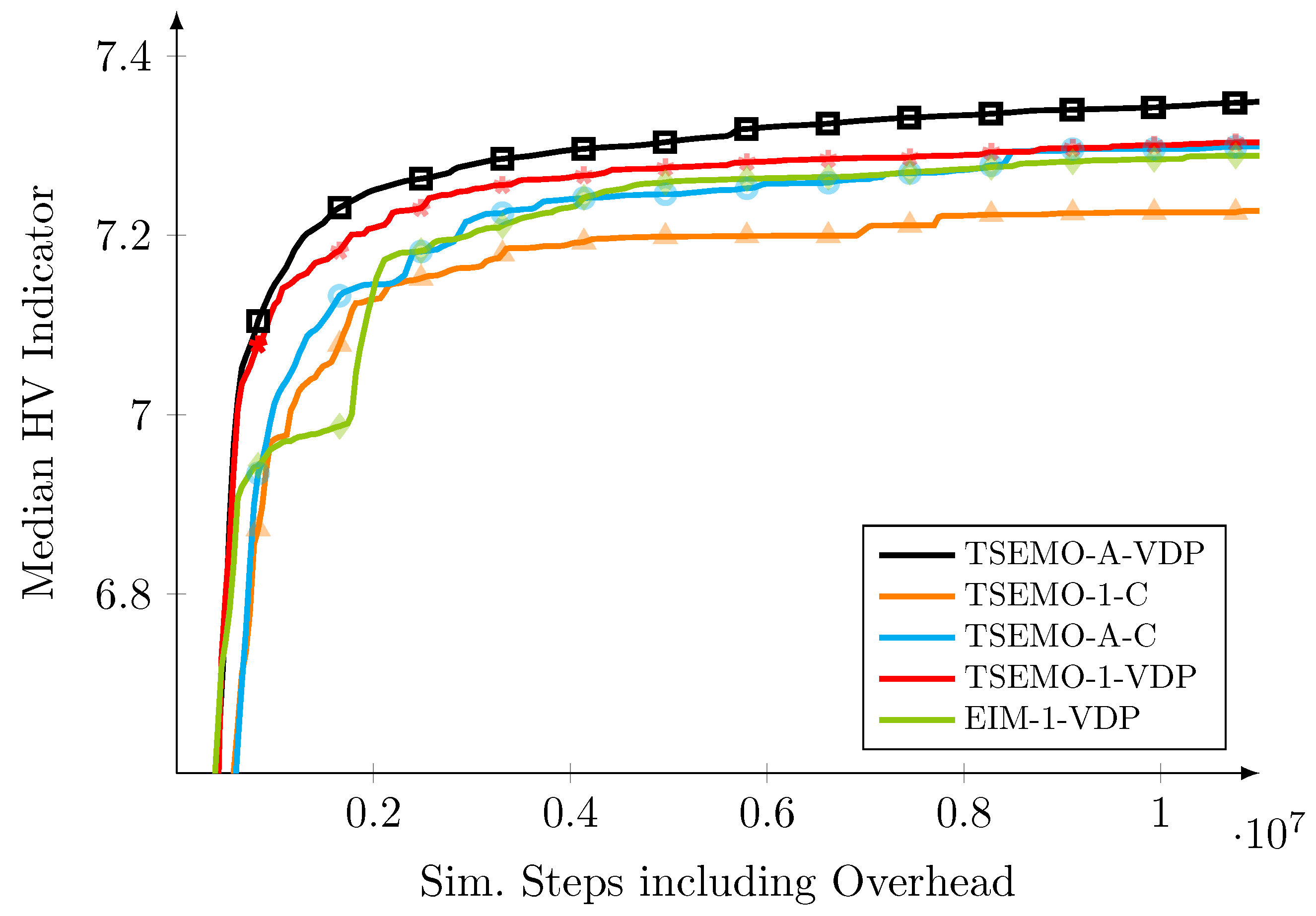
5.1. Evaluated Optimizers

In total, five different BO variants were evaluated:
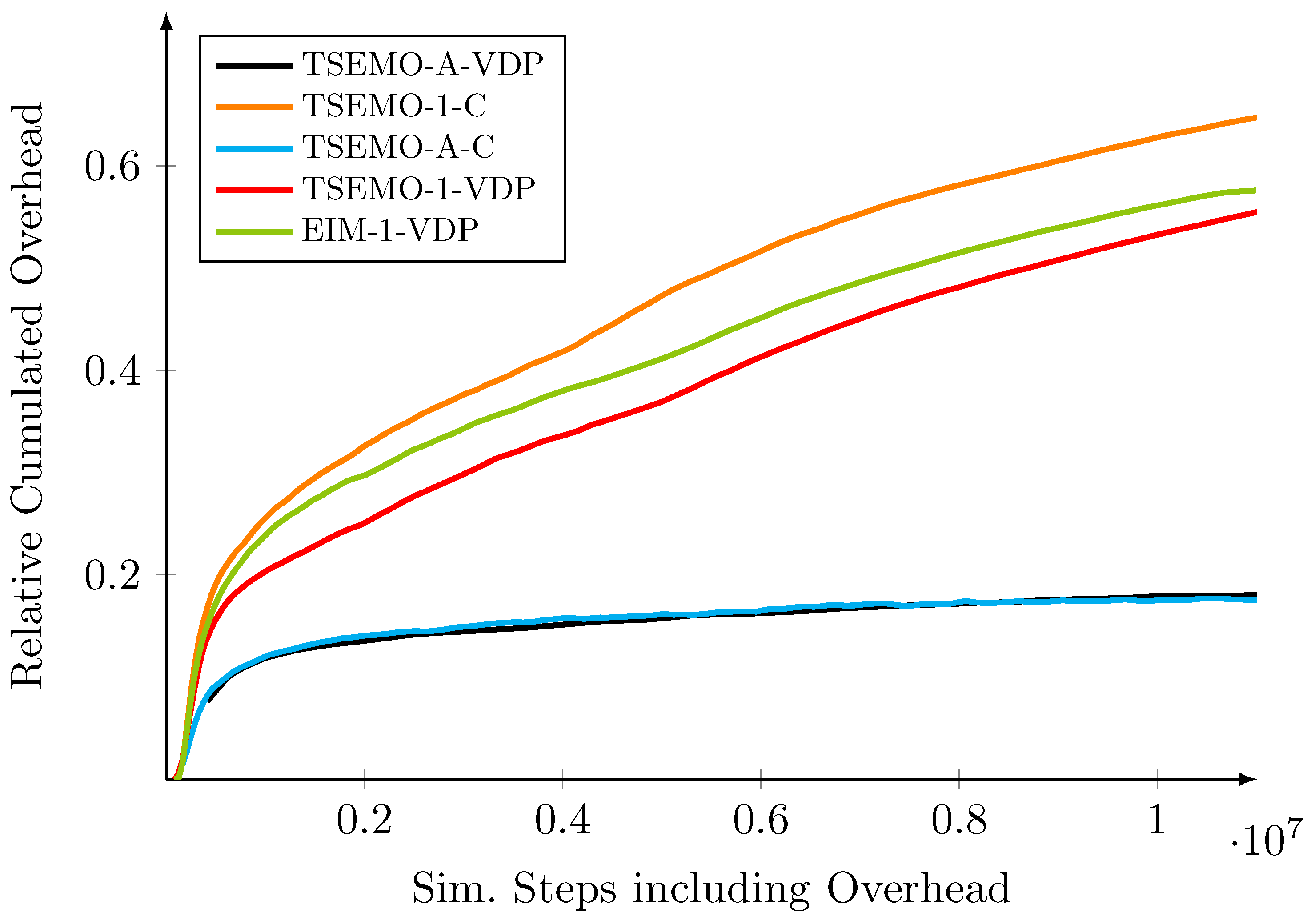
  • TSEMO-1-C: MOBO with TSEMO as the acquisition function and a constant batch size of one, without VDP.
  • TSEMO-A-C: MOBO with TSEMO as the acquisition function and a variable batch size, without VDP.
  • TSEMO-1-VDP: MOBO with TSEMO as the acquisition function and a constant batch size of one, with VDP.
  • TSEMO-A-VDP: MOBO with TSEMO as the acquisition function and a variable batch size, with VDP.
  • EIM-1-VDP: MOBO with EIM as the acquisition function and a constant batch size of one, with VDP.
If VDP (cf. Section 4.1.3) was not used, constant objective values were assigned to the failed evaluations. The BO variants were compared with NSGA-II and MOPSO. Random sampling (Rand) was performed as an additional benchmark by drawing parameterizations from a uniform distribution, bounded by the box constraints. Grid search (Grid) was used as the final benchmark. For grid search, each parameter θ i was discretized into six equally spaced levels. Based on this discretization, the parameter space was evaluated as a full factorial.

5.2. Metrics

The hypervolume (HV) indicator (e.g., [38]) was used as the primary performance metric. This is the most common metric for comparing multi-objective optimization algorithms [39]. To minimize the impact of initial sample quality on optimizer performance, each algorithm was run with ten different seeds. The median HV indicator was calculated from these runs and used to compare the different optimization approaches. In addition to comparing the median, a hypothesis test was used to evaluate the statistical significance of the differences. It cannot be assumed that the distribution of the HV indicator follows a Gaussian trend. Therefore, the non-parametric, one-sided Wilcoxon rank sum test was used with a significance level of 5%.
On average, one evaluation accounts for approximately 8.4e3 simulation time steps and takes around 20 seconds. The objective function evaluation time differs depending on the parameterization of the algorithm. Therefore, simulation steps were used to measure computational effort instead of objective function evaluations. In contrast to the evaluated metaheuristics, BO has a large overhead, caused by Steps 4–7 in Algorithm 1. Therefore, to evaluate the practical usability of the optimizers, it is not sufficient to only compare the computing effort of the objective function evaluations. Instead, the overhead was converted to equivalent simulation time steps by dividing the overhead time by the average time required for one simulation time step. The converted overhead was added to the simulation steps to obtain the total computing effort in terms of the simulation time steps.

5.3. Comparison of BO Variants

Figure 4 shows the progression of the HV indicator for the evaluated BO variants and a budget of 10 7 steps ( 1180 evals ) . It can be observed that TSEMO, with a flexible batch size and virtual datapoints to handle crash constraints (TSEMO-A-VDP), performs best. If a fixed budget of one evaluation per iteration is used (TSEMO-1-VDP), a decrease in performance can be observed with an increasing number of steps. After around 1.7 · 106 steps ( 200 evals ) , the difference is statistically significant. The same trend can be observed when comparing the BO variants TSEMO-A-C and TSEMO-1-C, which do not use VDP.
As an explanation, Figure 5 shows the overhead of the BO variants. It can be seen that the relative cumulative overhead is bounded to under 0.2 by adapting the batch size. Therefore, in this case, trading overhead for a potential reduction in sample quality is shown to be beneficial.
Additionally, using the adaptive VDP approach to deal with crashed simulations is significantly better than assigning a fixed objective function value. This can be observed for cases with an adaptive batch size and a batch size of one. Compared to TSEMO (TSEMO-1-VDP), the expected improvement matrix criterion (EIM-1-VDP) performed worse for the application at hand.

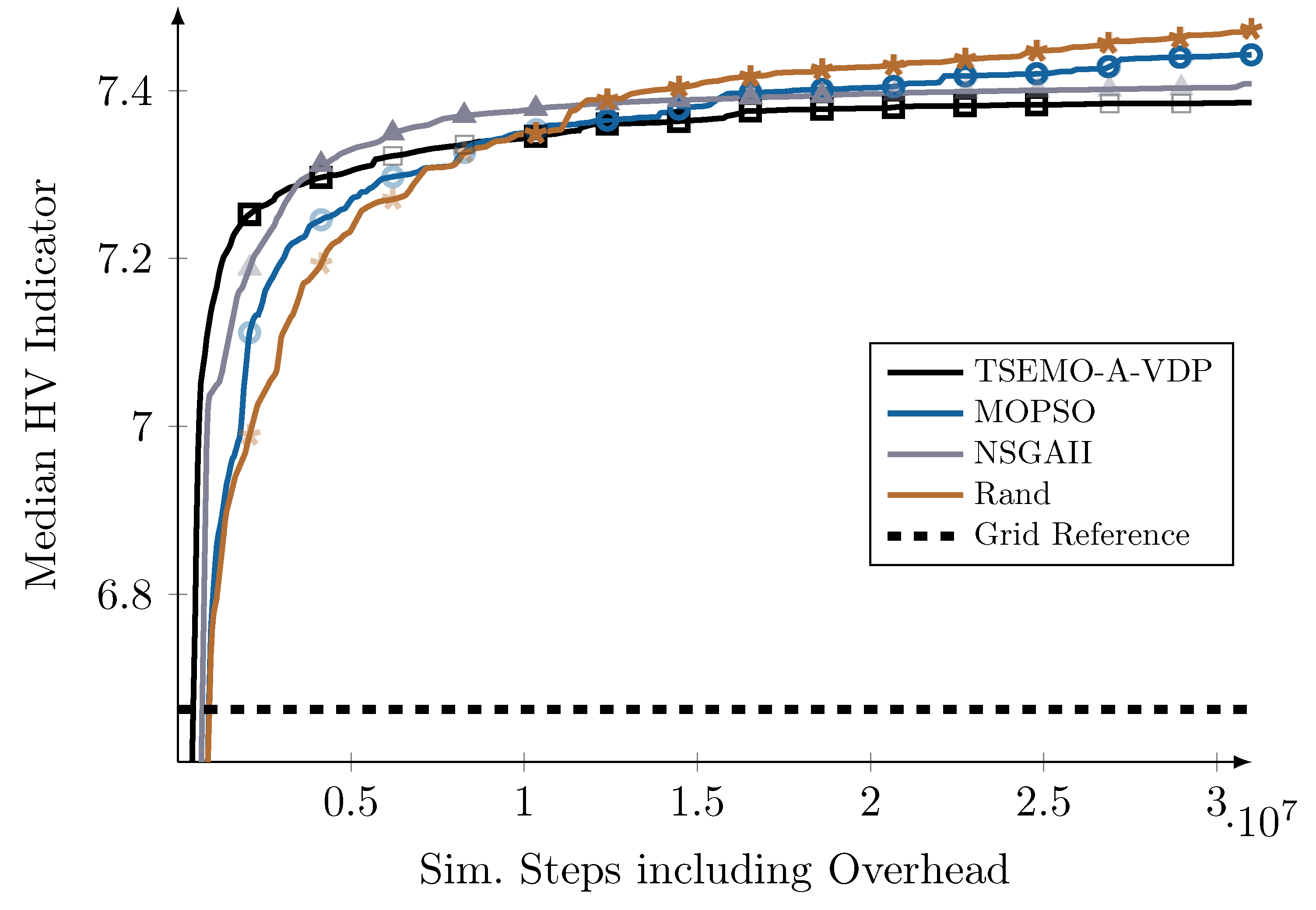
5.4. Overall Comparison

Figure 6 compares the best-performing BO variant with random sampling, grid search, NSGA-II, and MOPSO for a budget of 3.25 · 107 steps ( 3850 evals ) . For a small budget, i.e., until around 2.5 · 106 steps ( 294 evals ) , TSEMO-A-VDP performs statistically significantly better than the other optimizers. For a medium budget of around 8.0 · 106 steps ( 950 evals ) , NSGA-II is statistically significantly best. After around 1.2 · 107 steps ( 1430 evals ) , the median of random sampling (Rand) is best. MOPSO performs similarly to Rand, with slight advantages for a small-to-medium budget. However, in contrast to TSEMO-A-VDP and NSGA-II, MOPSO is not statistically significantly worse than Rand at the maximum budget. Importantly, TSEMO-A-VDP performs worse at the maximum budget, even if overhead is not taken into account (the corresponding plot is not shown here for briefness.) This indicates that, in addition to an increase in overhead, TSEMO may suffer a decrease in sample quality if a large amount of data have already been acquired.
All optimizers and random sampling quickly outperform grid search, although grid search requires a substantially higher computational effort, at 5.24 · 107 steps. This may indicate the low intrinsic dimensionality of the problem.

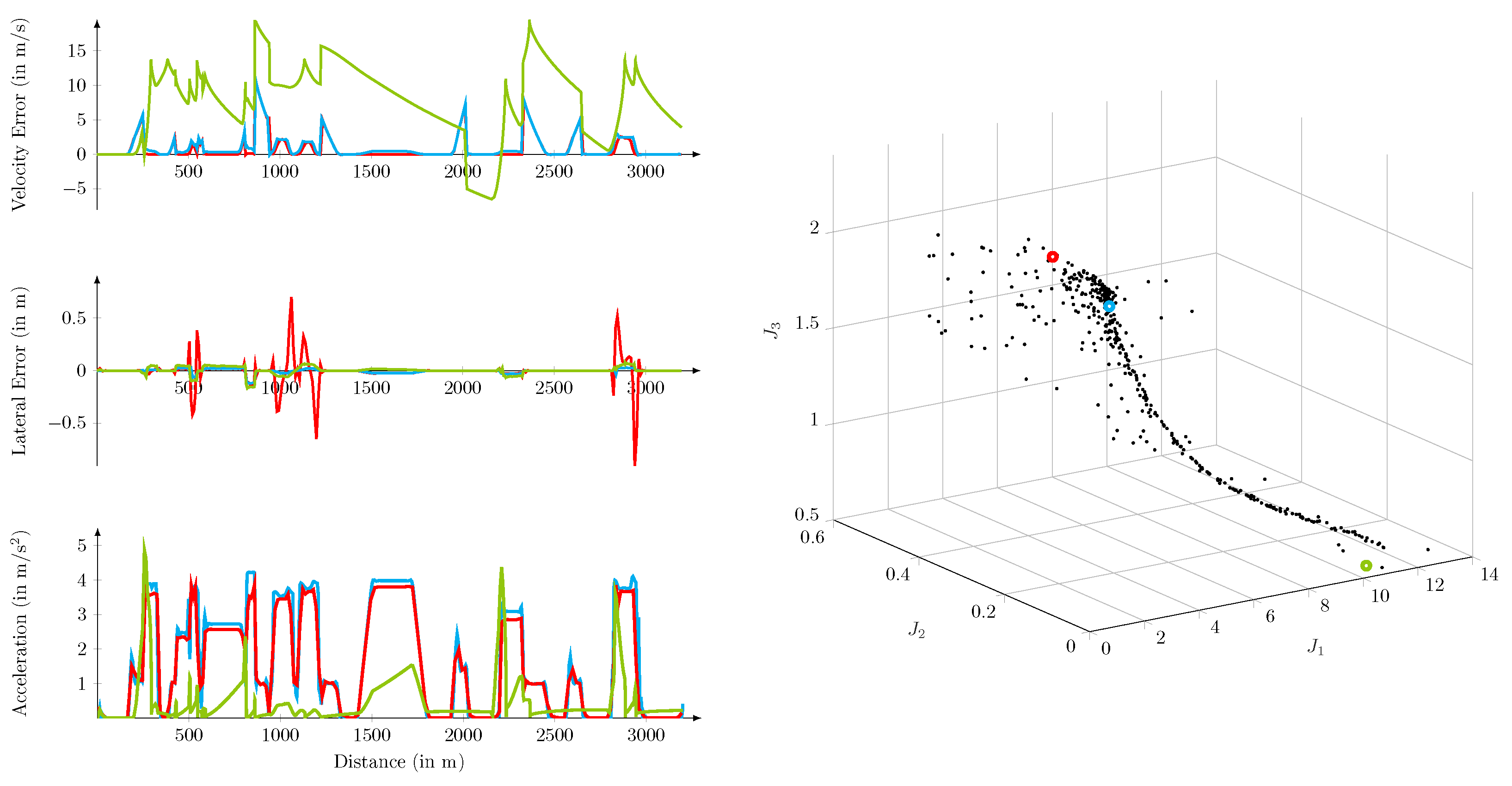
5.5. Practical Implications

Figure 7 provides an example of the time-domain behaviors of three different parameterizations belonging to the Pareto front. It can be observed that vastly different control behaviors can be achieved with different parameterizations. From a practical perspective, knowledge of the Pareto front and its corresponding parameterizations has many advantages. First, it enables the intuitive parameterization of the vehicle guidance system: application engineers can move on the Pareto front if they feel that the driving experience is too smooth or too rough. Users can also look up the corresponding optimal parameterizations without an in-depth understanding of the MPC itself or manually tune the parameters through numerous driving tests. In addition, the dimensionality of the application of vehicle guidance is significantly reduced in the case considered here, from five MPC parameters to three intuitive objectives. In other applications, this ratio can arbitrarily vary. This can significantly reduce the time required for its application.
Second, the optimization may find parameterizations that even an experienced engineer would not have tried: this may increase the control performance compared to manual tuning. Third, knowledge of the Pareto front makes it very easy to implement an automatic switching of MPC parameterization: this allows, for example, for a situation-dependent switching of the parameterization based on the objectives that are important for a particular situation. For instance, one could use a different parameterization on the highway (comfort is important) than when parking (tracking is important).

6. Conclusions

In this paper, we considered model predictive control (MPC) for the lateral and longitudinal control of autonomous vehicles, and compared the sample efficiency and the computational overhead of five different multi-objective Bayesian optimization (MOBO) versions and two metaheuristics, Multiple Objective Particle Swarm Optimization (MOPSO) and Non-dominated Sorting Genetic Algorithm II (NSGA-II). Multi-objective MPC tuning is shown to be capable of automatically finding parameters that produce versatile closed-loop behaviors. The presented method has two advantageous features. First, the problem of applying vehicle guidance is reduced from five dimensions in a parameter space to a two-dimensional manifold in three-dimensional objective function space. Second, the individual parameterizations represented by each point of this manifold can be interpreted very well by their resulting physical effects. The substantiality of the dimension reduction and the interpretability is determined by the respective application or the respective design.
From an optimization perspective, it was shown that, for this specific application, properly addressing crash constraints is essential to BO performance. Additionally, the overhead was bounded by adaptively choosing the sample size, increasing the overall optimization speed. Compared to other optimizers, BO was only best for a small number of objective function evaluations. For medium budgets, NSGA-II is best, and for large budgets, only MOPSO was not statistically significantly worse than random search. Grid search was clearly outperformed. Future work should address whether these findings carry over to other applications.

Author Contributions

Conceptualization, D.S., R.R. and R.V.; Methodology, D.S., R.R., R.V. and H.R.; Software, D.S., R.R., F.K. and R.V.; Formal analysis, D.S., R.R. and F.K.; Writing—original draft, D.S., R.R. and F.K.; Writing—review & editing, D.S., R.R., R.V. and H.R.; Supervision, R.V. and H.R. All authors have read and agreed to the published version of the manuscript.

Funding

This work was partially supported by the German Federal Ministry for Economic Affairs and Climate Action (BMWK) under the grant 50NA1912.

Data Availability Statement

Not applicable.

Conflicts of Interest

The authors declare no conflict of interest.

References

  1. Ulsoy, A.G.; Peng, H.; Çakmakci, M. Automotive Control Systems; Cambridge University Press: Cambridge, MA, USA, 2012. [Google Scholar] [CrossRef]
  2. Kiencke, U.; Nielsen, L. Automotive Control Systems: For Engine, Driveline, and Vehicle; Springer: Berlin/Heidelberg, Germany, 2005. [Google Scholar]
  3. Isermann, R. Automotive Control: Modeling and Control of Vehicles; ATZ/MTZ-Fachbuch, Springer: Berlin/Heidelberg, Germany, 2022. [Google Scholar]
  4. No, T.S.; Chong, K.T.; Roh, D.H. A Lyapunov function approach to longitudinal control of vehicles in a platoon. In Proceedings of the IEEE 51st Conference on Vehicular Technology (VTC2000), Tokyo, Japan, 15–18 May 2000; Volume 1, pp. 336–340. [Google Scholar] [CrossRef]
  5. Liaw, D.C.; Chung, W.C. A Feedback Linearization Design for the Control of Vehicle’s Lateral Dynamics. Nonlinear Dyn. 2008, 52, 313–329. [Google Scholar] [CrossRef]
  6. Zhang, S.; Zhou, S.; Sun, J. Vehicle dynamics control based on sliding mode control technology. In Proceedings of the 2009 Chinese Control and Decision Conference, Shanghai, China, 16–18 December 2009; pp. 2435–2439. [Google Scholar] [CrossRef]
  7. Hrovat, D.; Di Cairano, S.; Tseng, H.; Kolmanovsky, I. The development of Model Predictive Control in automotive industry: A survey. In Proceedings of the 2012 IEEE International Conference on Control Applications, Dubrovnik, Croatia, 3–5 October 2012; pp. 295–302. [Google Scholar] [CrossRef]
  8. Feng, G.; Han, Y.; Li, S.E.; Xu, S.; Dang, D. Accurate Pseudospectral Optimization of Nonlinear Model Predictive Control for High-performance Motion Planning. IEEE Trans. Intell. Veh. 2022. [Google Scholar] [CrossRef]
  9. Yamashita, A.; Zanin, A.; Odloak, D. Tuning of model predictive control with multi-objective optimization. Braz. J. Chem. Eng. 2016, 33, 333–346. [Google Scholar] [CrossRef]
  10. Shah, G.; Engell, S. Tuning MPC for desired closed-loop performance for MIMO systems. In Proceedings of the 2011 American Control Conference, San Francisco, CA, USA, 29 June–1 July 2011; pp. 4404–4409. [Google Scholar] [CrossRef]
  11. Vega, P.; Francisco, M.; Sanz, E. Norm based approaches for automatic tuning of Model Based Predictive Control. In Proceedings of the European Congress of Chemical Engineering, Copenhagen, Denmark, 16–20 September 2007; pp. 1–10. [Google Scholar]
  12. Al-Ghazzawi, A.; Ali, E.; Nouh, A.; Zafiriou, E. On-line tuning strategy for model predictive controllers. J. Process Control 2001, 11, 265–284. [Google Scholar] [CrossRef]
  13. Stenger, D.; Ay, M.; Abel, D. Robust Parametrization of a Model Predictive Controller for a CNC Machining Center Using Bayesian Optimization. IFAC-PapersOnLine 2020, 53, 10388–10394. [Google Scholar] [CrossRef]
  14. Ramasamy, V.; Sidharthan, R.; Kannan, R.; Muralidharan, G. Optimal Tuning of Model Predictive Controller Weights Using Genetic Algorithm with Interactive Decision Tree for Industrial Cement Kiln Process. Processes 2019, 7, 938. [Google Scholar] [CrossRef] [Green Version]
  15. Marco, A.; Baumann, D.; Khadiv, M.; Hennig, P.; Righetti, L.; Trimpe, S. Robot Learning With Crash Constraints. IEEE Robot. Autom. Lett. 2021, 6, 1439–1446. [Google Scholar] [CrossRef]
  16. Stenger, D.; Abel, D. Benchmark of Bayesian Optimization and Metaheuristics for Control Engineering Tuning Problems with Crash Constraints. arXiv 2022, arXiv:2211.02571. [Google Scholar]
  17. Ryo, A.; Matthew, T.; Kenta, K.; Howie, C.; Fumitoshi, M. Multiobjective Optimization Based on Expensive Robotic Experiments under Heteroscedastic Noise. IEEE Trans. Robot. 2017, 33, 468–483. [Google Scholar] [CrossRef]
  18. Matthew, T.; Jeff, S.; Howie, C. Expensive multiobjective optimization for robotics. In Proceedings of the 2013 IEEE International Conference on Robotics and Automation, Karlsruhe, Germany, 6–10 May 2013; pp. 973–980. [Google Scholar] [CrossRef]
  19. Matteo, T.; Andreas, K.; Sebastian, T. Robust Model-free Reinforcement Learning with Multi-objective Bayesian Optimization. In Proceedings of the 2020 IEEE International Conference on Robotics and Automation (ICRA), Paris, France, 31 May–31 August 2020; pp. 10702–10708. [Google Scholar] [CrossRef]
  20. Kim, Y.; Pan, Z.; Hauser, K.K. MO-BBO: Multi-Objective Bilevel Bayesian Optimization for Robot and Behavior Co-Design. In Proceedings of the 2021 IEEE International Conference on Robotics and Automation (ICRA), Xi’an, China, 30 May–5 June 2021; pp. 9877–9883. [Google Scholar]
  21. Gharib, A.; Stenger, D.; Ritschel, R.; Voßwinkel, R. Multi-Objective Optimization of a Path-following MPC for Vehicle Guidance: A Bayesian Optimization Approach. In Proceedings of the 2021 European Control Conference (ECC), Virtual, 29 June–2 July 2021; pp. 2197–2204. [Google Scholar] [CrossRef]
  22. Emmerich, M.; Klinkenberg, J.W.; Bohrweg, N. The Computation of the Expected Improvement in Dominated Hypervolume of Pareto Front Approximations; Rapport Technique: Leiden, The Netherlands, 2008; Available online: https://liacs.leidenuniv.nl/~emmerichmtm/moda/material/TR-ExI.pdf (accessed on 10 January 2023).
  23. Zhan, D.; Cheng, Y.; Liu, J. Expected Improvement Matrix-Based Infill Criteria for Expensive Multiobjective Optimization. IEEE Trans. Evol. Comput. 2017, 21, 956–975. [Google Scholar] [CrossRef]
  24. Bradford, E.; Schweidtmann, A.M.; Lapkin, A. Efficient multiobjective optimization employing Gaussian processes, spectral sampling and a genetic algorithm. J. Glob. Optim. 2018, 71, 407–438. [Google Scholar] [CrossRef] [Green Version]
  25. Ritschel, R.; Schrödel, F.; Hädrich, J.; Jäkel, J. Nonlinear Model Predictive Path-Following Control for Highly Automated Driving. In Proceedings of the 10th IFAC Symposium on Intelligent Autonomous Vehicles IAV 2019, Gdansk, Poland, 3–5 July 2019; Volume 52, pp. 350–355. [Google Scholar] [CrossRef]
  26. Faulwasser, T. Optimization-Based Solutions to Constrained Trajectory-Tracking and Path-Following Problems; Shaker Verlag: Aachen, Germany, 2013. [Google Scholar]
  27. Wang, C.; Zhao, X.; Fu, R.; Li, Z. Research on the Comfort of Vehicle Passengers Considering the Vehicle Motion State and Passenger Physiological Characteristics: Improving the Passenger Comfort of Autonomous Vehicles. Int. J. Environ. Res. Public Health 2020, 17, 6821. [Google Scholar] [CrossRef] [PubMed]
  28. Shahriari, B.; Swersky, K.; Wang, Z.; Adams, R.P.; de Freitas, N. Taking the Human Out of the Loop: A Review of Bayesian Optimization. Proc. IEEE 2016, 104, 148–175. [Google Scholar] [CrossRef] [Green Version]
  29. Rasmussen, C.E.; Williams, C.K.I. Gaussian Processes for Machine Learning (Adaptive Computation and Machine Learning); The MIT Press: Cambridge, MA, USA, 2005. [Google Scholar]
  30. Deb, K.; Agrawal, S.; Pratap, A.; Meyarivan, T. A fast and elitist multiobjective genetic algorithm: NSGA-II. IEEE Trans. Evol. Comput. 2002, 6, 182–197. [Google Scholar] [CrossRef] [Green Version]
  31. Schweidtmann, A. Multi-Objective Optimization Algorithm for Expensive-to-Evaluate Function. 2019. Available online: https://github.com/Eric-Bradford/TS-EMO (accessed on 10 December 2021).
  32. Stenger, D.; Nitsch, M.; Abel, D. Joint Constrained Bayesian Optimization of Planning, Guidance, Control, and State Estimation of an Autonomous Underwater Vehicle. In Proceedings of the 2022 European Control Conference (ECC), London, UK, 11–14 July 2022; pp. 1982–1987. [Google Scholar] [CrossRef]
  33. Kato, K.; Ariizumi, R.; Matsuno, F. Multiobjective Optimization Method for Expensive Functions with Unknown Failure Regions and Its Application to Mobile Robot. J. Robot. Soc. Jpn. 2017, 35, 143–152. [Google Scholar] [CrossRef] [Green Version]
  34. Branke, J.; Deb, K.; Miettinen, K.; Slowinski, R. Multiobjective Optimization; The MIT Press: Cambridge, MA, USA, 2008. [Google Scholar]
  35. Martínez-Cagigal, V. Multi-Objective Particle Swarm Optimization (MOPSO). Version 1.3.2.0. 2019. Available online: https://www.mathworks.com/matlabcentral/fileexchange/62074-multi-objective-particle-swarm-optimization-mopso (accessed on 28 May 2022).
  36. Coello, C.A.C.; Pulido, G.T.; Lechuga, M.S. Handling multiple objectives with particle swarm optimization. IEEE Trans. Evol. Comput. 2004, 8, 256–279. [Google Scholar] [CrossRef]
  37. Sierra, M.R.; Coello Coello, C.A. Improving PSO-Based Multi-objective Optimization Using Crowding, Mutation and ϵ-Dominance. In Evolutionary Multi-Criterion Optimization, EMO 2005; Coello Coello, C.A., Hernández Aguirre, A., Zitzler, E., Eds.; Springer: Berlin/Heidelberg, Germany, 2005; pp. 505–519. [Google Scholar]
  38. Guerreiro, A.P.; Fonseca, C.M.; Paquete, L. The Hypervolume Indicator: Computational Problems and Algorithms. ACM Comput. Surv. 2021, 54, 1–42. [Google Scholar] [CrossRef]
  39. Riquelme, N.; Von Lücken, C.; Baran, B. Performance metrics in multi-objective optimization. In Proceedings of the 2015 Latin American Computing Conference (CLEI), Arequipa, Peru, 19–23 October 2015; pp. 1–11. [Google Scholar] [CrossRef]
Figure 1. Controller tuning framework consisting of the simulation environment (depicted in blue) and the parameter optimizer (depicted in orange). The parameter optimizer uses simulation data from the simulation environment to produce a specific parameter vector θ , used in the MPC. For a detailed view of the MPC implementation and the variables involved, see Figure 2.
Mathematics 11 00465 g001
Figure 2. MPC implementation for longitudinal and lateral vehicle control based on a model predictive path-following control (MPFC) approach. Based on a specific parameter vector θ , the reference path p ( s ) and the desired velocity v des the MPFC yields the target acceleration a set and the steering wheel target angular velocity ω s , set (and, subsequently, the steering wheel target angle δ s , set ), which are used as an input to the vehicle model.
Mathematics 11 00465 g002
Figure 3. 2D view of the target line and the speed limit v l i m of the circular track used in the simulation. The different sections of the target line are highlighted by the colors cyan and orange for clarity.
Mathematics 11 00465 g003
Figure 4. HV indicator as a function of simulation steps including algorithmic overhead. Markers in light colors indicate that the HV indicator of the respective algorithm is statistically significantly worse than the best BO variant.
Mathematics 11 00465 g004
Figure 5. Relative cumulative overhead (c.f. Section 5.2) of the BO variants. The overhead of Rand, NSGA-II and MOPSO are not shown because they are very small < 0.01 .
Mathematics 11 00465 g005
Figure 6. HV indicator as a function of simulation steps, including algorithmic overhead. Markers in light colors indicate that the HV indicator of the respective algorithm is statistically significantly worse than the best-performing optimizer.
Mathematics 11 00465 g006
Figure 7. (Left) Time-domain plot for three different Pareto-optimal MPC parameterizations. The green, blue and red parameterizations focus on minimizing acceleration, lateral error, and velocity error, respectively. (Right) Corresponding objective Pareto front, where the parameterizations shown in the left image are marked in the equivalent colors: minimizing acceleration (green dots), lateral error (blue dots) and velocity (red dots). All other parameterizations on the Pareto front (black dots) represent alternative non-dominated compromises.
Mathematics 11 00465 g007
Disclaimer/Publisher’s Note: The statements, opinions and data contained in all publications are solely those of the individual author(s) and contributor(s) and not of MDPI and/or the editor(s). MDPI and/or the editor(s) disclaim responsibility for any injury to people or property resulting from any ideas, methods, instructions or products referred to in the content.

