The Optical Path Method for the Problem of Oblique Incidence of a Plane Electromagnetic Wave on a Plane-Parallel Scatterer

Abstract

A number of actual problems of integrated photonics are reduced to an oblique incidence of radiation on a plane-parallel scatterer. For such problems, an approximate method of integrating the Maxwell equations along the beam propagation direction is proposed. As a result, the original two-dimensional problem is reduced to a one-dimensional one, and recently proposed one-dimensional bicompact schemes are used to solve it. This approach provides a significant reduction of computational costs compared to traditional two-dimensional methods such as finite differences and finite elements. To verify the proposed method, calculations of test and applied problems with known exact reflection spectra are carried out.

1. Introduction

Integrated photonics is the field of optics dedicated to the development of nanoscale devices that allow controlling radiation in the near-infrared and visible range. Optical nanostructures can be used as detectors, logic elements, switches, modulators, waveguides, etc. A number of important applications are reduced to the problem of oblique incidence of a plane electromagnetic wave (monochromatic or pulse) on a set of plane-parallel plates. The latter can be both dielectric and conductive, and their material parameres may depend on the coordinates. Such problems arise when studying the properties of bound states of various types (surface [1] or Tamm [2,3] plasmon polaritons, micro-cavity modes [4], excitons [5], etc.).

The outlined problems are two-dimensional; i.e., electromagnetic fields depend on two spatial coordinates, and the dependence on the third coordinate can be neglected. For such problems, two-dimensional codes based on the finite difference or finite element method are traditionally used.

For monochromatic problems in the absence of surface currents, the methods of finite and boundary elements based on the Raviar-Thomas [6] and Nedelec [7] elements seem to be the most workable.

For non-stationary problems, finite difference, finite element, and finite volume methods in the time domain are only applicable [8,9,10,11]. However, these methods face a number of difficulties [12]. Firstly, near the interface of the media, the error turns out to be large. Secondly, real optical media have frequency dispersion. Existing methods of accounting for it may introduce a noticeable error in the solution.

If the fields are monochromatic, and the media are dielectric and piecewise homogeneous, then scattering matrix methods [13] are used. These methods provide not an approximate but an exact solution to the problem. Within their scope of applicability, these methods are the most workable. Sveshnikov and Tikhonravov generalized the scattering matrix method to problems in layered media with spatially inhomogeneous layers [14]; however, this generalization is applicable only for normal radiation incidence.

In some cases, with the help of physical approximations, the problem can be simplified and reduced to a one-dimensional formulation (see, e.g., [15,16,17,18,19,20,21,22,23]). This greatly simplifies the calculation. An example is the integration of hyperbolic problems along the direction of wave propagation. However, most of such approaches are developed for cases when there are no interface boundaries in the medium; i.e., the properties of the substance change smoothly in space. At the same time, a characteristic feature of integrated photonics problems is the presence of several interface boundaries on which multiple re-reflections occur.

In the present paper, we propose to integrate the Maxwell equations along the direction of wave propagation. This approach reduces the problem to a one-dimensional one. For the latter, a recently proposed bicompact scheme and the spectral decomposition method are used. This allows us to reduce the complexity of solving the tasks listed above. Calculations of test and applied problems with a known exact reflection spectra have been carried out, which convincingly verify the proposed approach.

2. Problem Statement

2.1. Plane-Parallel Structure

1. Consider a layered structure consisting of Q isotropic plane-parallel plates with a total thickness of a. Let the coordinate axis z be perpendicular to the plates; the axes x and y are located in the plane of the plates. Denote the coordinates of the layer boundaries by $0={\xi }_0<{\xi }_1<\dots <{\xi }_Q=a$. At $z<0$ and $z>a$, semi-infinite dielectric media are located. We denote their dielectric permittivity and magnetic susceptibility by ${\epsilon }_0$, ${\mu }_0$ (for $z<0$) and ${\epsilon }_a$, ${\mu }_a$ (for $z>a$). We assume these media to be homogeneous and isotropic.

2. Let part of the plates be dielectric and part of them be conductors or semiconductors. Denote by ${\epsilon }_q$ the dielectric permittivity, ${\mu }_q$ the magnetic susceptibility, and ${\sigma }_q$ the conductivity of the q th plate (for dielectric plates, ${\sigma }_q=0$).

3. Due to heating by currents and incident radiation, the plates may become optically inhomogeneous, that is, their refractive index may depend on the coordinate. We assume that the refractive index and conductivity depend on the z coordinate but practically do not change with time.

4. The values ${\epsilon }_q$, ${\mu }_q$, ${\sigma }_q$ may depend on the frequency $\omega$ of the electromagnetic wave. This dispersion is called the frequency one. At the same time, we assume that the spatial dispersion (i.e., the dependence of the material parameters on the wave vector) is negligible.

Note that in the presence of spatial dispersion, the wavefront is deformed (and cannot be considered homogeneous). Polarization deformation occurs, which may lead to the implementation of multimode oscillations, waveguide modes, etc. [24]. This class of tasks is beyond the scope of this work.

Spatial dispersion is insignificant if the field changes little at the distance at which the response of the medium to this field is formed [24]. The change in the field occurs due to the displacement of charges in the substance. Thus, we assume that the displacement of charges during the oscillation period of the fields is small compared to the wavelength. In plasma physics problems, this means the approximation of a cold plasma. In problems of dielectric photonics and plasmonics, this approximation is applicable because the frequency of field oscillations is high. Thus, the typical oscillation period in the optical and near-infrared range is $\sim {10}^{-14}$ s. During this time, the free electrons in the metal shift by the fractions of an angstrom, while the characteristic wavelength is hundreds of nanometers.

2.2. Scattering of Monochromatic Radiation by Plasmonic Structures

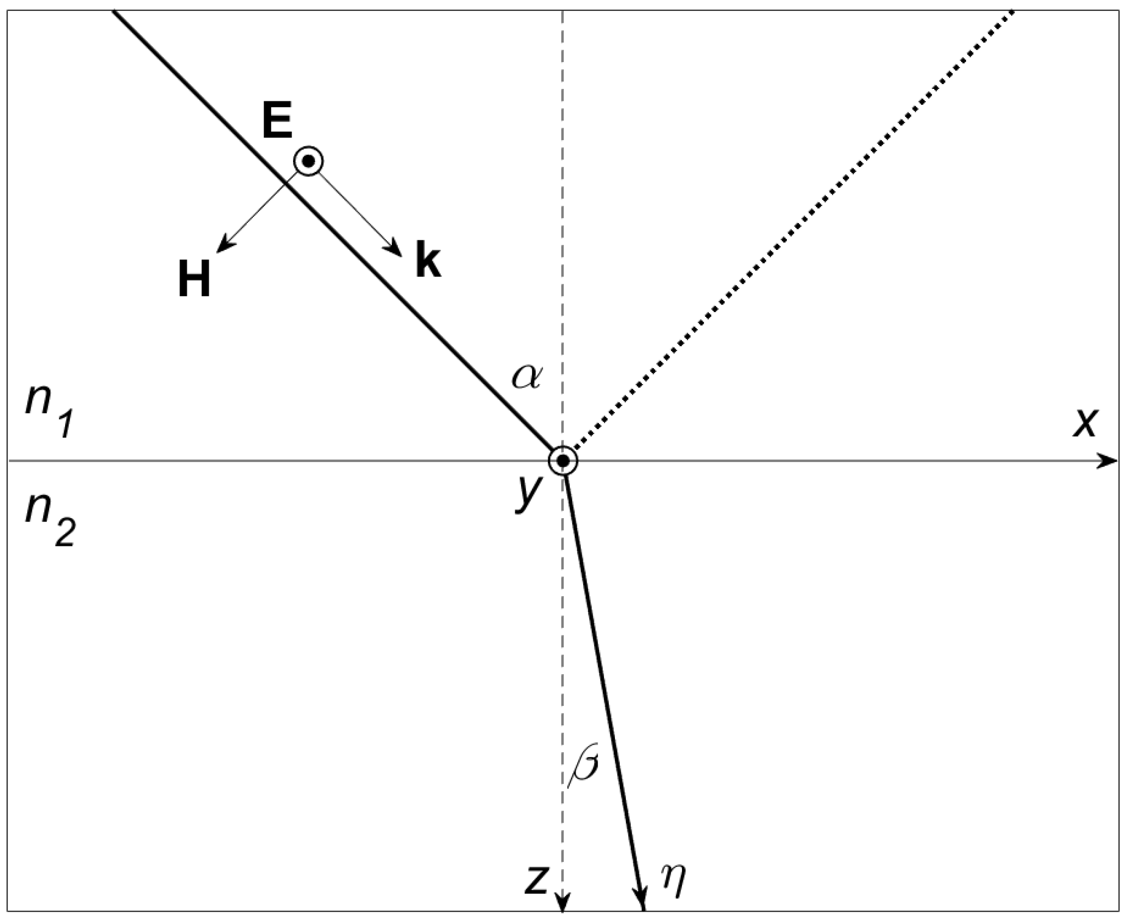
1. Let a plane linearly polarized electromagnetic wave of frequency $\omega$ fall obliquely on the structure and the wave vector lie in the $Oxz$ plane. The angle of incidence (i.e., the angle between the wave vector of the incident wave and the normal to the plates) is denoted by $\alpha$.

It is known that two wave polarizations are possible for oblique incidence. A wave is called s-polarized if the vector $\mathbf{E}$ is perpendicular to the plane formed by the wave vectors of the incident and reflected waves. Then, the vector $\mathbf{E}$ has only y-component $\mathbf{E}=\{0,E_y,0\}$, and the vector $\mathbf{H}$ has x- and z-components $\mathbf{H}=\{H_x,0,H_z\}$. This polarization is illustrated in Figure 1, where one media interface is given for simplicity. If the vector $\mathbf{E}$ lies in the plane formed by the wave vectors of the incident and reflected waves, then the wave is called p-polarized (see Figure 2). Then, the vector $\mathbf{E}$ has x- and z-components $\mathbf{E}=\{E_x,0,E_z\}$, and the vector $\mathbf{H}$ has only y-component $\mathbf{H}=\{0,H_y,0\}$.

Moreover, if the incident wave has s-polarization, then the reflected and transmitted waves are also s-polarized, and it is similar in the case of p-polarization. We assume that the incident wave is s- or p-polarized. It is this case that is of interest to applications.

If the incident wave has a circular or elliptical polarization, then it can be represented as the sum of two linear polarizations (s and p). Next, one solves the problem for each of them and sums up the answer.

2. Suppose there are no external bulk currents ${\mathbf{J}}^{\mathrm{ext}}=0$. Incident radiation induces bulk currents ${\mathbf{J}}_q^{\mathrm{ind}}={\sigma }_q{\mathbf{E}}_q$. They are directed in the same way as the vector $\mathbf{E}$. These currents emit waves that interfere with the incident, reflected and transmitted waves. In this case, various bound states of the electromagnetic field can be formed.

3. We assume that the material of the plates may be inhomogeneous (e.g., due to heating by currents and incident radiation). In this case, we assume that ${\epsilon }_q$, ${\mu }_q$, ${\sigma }_q$ depend only on z and do not depend on x, y.

The described formulation arises in plasmonics [25,26,27]. It is often found in physical and technical applications: sensing, microscopy, optical communication, etc.

2.3. Scattering of Monochromatic Radiation by Optical Structures

1. In the problem, formulated in Section 2.2, all plates are made of dielectric materials and transparent to incident radiation (i.e., the value of $\mathrm{Im}\epsilon \ll 1$ is small). Let all bulk and surface currents be absent $J_q^{\mathrm{ext}}=J_q^{\mathrm{ind}}=0$, $j_q^{\mathrm{ext}}=j_q^{\mathrm{ind}}=0$.

2. Let a plane linearly polarized electromagnetic wave of frequency $\omega$ fall obliquely on this structure. We choose the direction of the coordinate axes in the same way as in the problem from Section 2.2. The incident radiation is partially reflected from the structure and partially passes through it. Bound states can be formed inside the structure, e.g., the Bloch surface waves [28,29].

3. The plates are spatially homogeneous, i.e., inside each plate, the material parameters ${\epsilon }_q$, ${\mu }_q$ are constant. Heating of the plates by incident radiation is supposed to be negligible.

4. In references, this problem is commonly called optical. It is found in many technical applications. Examples are reflectionless and antireflective coatings, planar waveguides, etc. (see, for example, [30,31]).

2.4. Scattering of an Electromagnetic Pulse by Plasmonic Structures

1. In the problem from Section 2.2, a monochromatic wave does not fall on the scatterer, but a wave packet

$${\mathbf{f}}^0\left(\zeta \right)={\mathbf{E}}^0\left(\zeta \right)exp\left(-i{\omega }^0\zeta \right),\zeta =t-\frac{({\tilde{\mathbf{k}}}^0\mathbf{r})}{{\tilde{k}}^{0}c}$$

(1)

with given carrier frequency ${\omega }^0$ and envelope ${\mathbf{E}}^0$. Here, ${\tilde{\mathbf{k}}}^0/{\tilde{k}}^0$ is a unit vector in the direction of wave propagation, $k^0={\omega }^0/c$. Let the pulse (1) be plane and linearly polarized, and the envelope is a finite function. We select the coordinate axes in the same way as in the problem (Section 2.2).

The incident radiation induces bulk currents ${\mathbf{J}}_q^{\mathrm{ind}}={\sigma }_q{\mathbf{E}}_q$, which re-emit linearly polarized pulses.

2. We assume that the refractive index and conductivity depend on the z coordinate but change slowly over time. The media have a frequency dispersion, but the spatial dispersion is negligible. The conditions when these assumptions are correct are formulated above.

3. The described problem arises when considering ultrafast processes in plasmon structures.

2.5. Scattering of an Electromagnetic Pulse by Optical Structures

1. Let a wave packet (1) fall on the scatterer in the problem from Section 2.3. We select the coordinate axes in the same way as in Section 2.3. The material parameters ${\epsilon }_q$, ${\mu }_q$ are assumed to be constant within each plate. There is a frequency dispersion, and the spatial dispersion is considered negligible.

2. This problem is of great importance for studying the dynamics of bound states in dielectric structures.

3. Problem in Integral Form

3.1. Stationary Case

The basic equations of electrodynamics are Maxwell’s equations. Traditionally, their differential form is considered in the literature. We use the integral form of these equations. For the case of monochromatic fields, these equations are as follows:

$$\begin{array}{c}{\int }_{\mathsf{\Gamma }}{\mathbf{H}}_{q}d\mathbf{l}=\frac{4\pi }{c}{\int }_S{\sigma }_q{\mathbf{E}}_{q}d\mathbf{s}-\frac{i\omega }{c}{\int }_S{\mathbf{D}}_{q}d\mathbf{s},{\mathbf{D}}_q={\epsilon }_q{\mathbf{E}}_q,1\le q\le Q;\end{array}$$

(2)

$$\begin{array}{c}{\int }_{\mathsf{\Gamma }}{\mathbf{E}}_{q}d\mathbf{l}=\frac{i\omega }{c}{\int }_S{\mathbf{B}}_{q}d\mathbf{s},{\mathbf{B}}_q={\mu }_q{\mathbf{H}}_q,1\le q\le Q.\end{array}$$

(3)

Here, S is an arbitrary surface bounded by the contour $\mathsf{\Gamma }$. The CGS system of units is used.

Let us formulate the radiation conditions for this problem. Consider a section of the scatterer bounded by the planes $x=0$ and $x=d>0$. For the compactness of the notation, we introduce the following designations:

$$A_q^{\pm }=\frac{\partial }{\partial x}\pm i{({\tilde{k}}_q)}_x,B_q^{\pm }=\frac{\partial }{\partial z}\pm i{({\tilde{k}}_q)}_z.$$

(4)

Here, ${({\tilde{k}}_q)}_x={\tilde{k}}_{q}sin{\alpha }_q$ and ${({\tilde{k}}_q)}_z={\tilde{k}}_{q}cos{\alpha }_q$ are projections of the wave vector in the qth plate on the x and z axes, respectively. The values of $1⩽q⩽Q-1$ correspond to the scatterer plates, $q=0$ is for medium at $z<0$, $q=Q$ is for medium at $z>a$. Recall that the wave number in the qth plate is equal to ${\tilde{k}}_q=\omega \sqrt{{\epsilon }_q{\mu }_q}/c$.

The operator $A_q^{+}{B}_q^{+}$ permits one to select the incident wave $\sim exp\{i{({\tilde{k}}_q)}_{x}x+i{({\tilde{k}}_q)}_{z}z\}$ in the qth medium and set its amplitude without affecting the amplitude of the reflected wave $\sim exp\{i{({\tilde{k}}_q)}_{x}x-i{({\tilde{k}}_q)}_{z}z\}$.

Thus, the radiation conditions take the following form:

$$\begin{array}{c}{A}_q^{+}{B}_q^{+}\mathbf{E}=-4{({\tilde{k}}_q)}_x{({\tilde{k}}_q)}_z{\mathbf{E}}_q^0{e}^{i{({\tilde{k}}_q)}_{z}z},x=0,{\xi }_{q-1}<z<{\xi }_q,\end{array}$$

(5)

$$\begin{array}{c}{A}_0^{+}{B}_0^{+}\mathbf{E}=-4{({\tilde{k}}_0)}_x{({\tilde{k}}_0)}_z{\mathbf{E}}_0^0{e}^{i{({\tilde{k}}_0)}_{z}z},z=0,0<x<d,\end{array}$$

(6)

$$\begin{array}{c}{A}_q^{-}{B}_q^{+}\mathbf{E}=0,x=d,{\xi }_{q-1}<z<{\xi }_q,\end{array}$$

(7)

$$\begin{array}{c}{A}_Q^{+}{B}_Q^{-}\mathbf{E}=0,z=a,0<x<d.\end{array}$$

(8)

Here, ${\mathbf{E}}_q^0$ is the amplitude of the wave incident on the interface $z={\xi }_q$ from the medium q to the medium $q+1$. The amplitude of ${\mathbf{E}}_{q+1}^0$ is related to ${\mathbf{E}}_q^0$ by the Fresnel coefficients. The amplitude ${\mathbf{E}}_0^0$ corresponds to the radiation incident on the boundary of the scatterer $z=0$. The conditions (7) show that the incident and reflected waves freely pass through the boundary $x=d$, and the condition (8) shows that the transmitted wave freely passes through the boundary $z=a$.

At the media interfaces, we set the conjugation conditions

$$\begin{array}{c}\begin{array}{cc}{\mathbf{e}}_z\times ({\mathbf{E}}_q-{\mathbf{E}}_{q-1})=0,\hfill & {\mathbf{e}}_z({\mathbf{D}}_q-{\mathbf{D}}_{q-1})=0,\hfill \\ {\mathbf{e}}_z\times ({\mathbf{H}}_q-{\mathbf{H}}_{q-1})=0,\hfill & {\mathbf{e}}_z({\mathbf{B}}_q-{\mathbf{B}}_{q-1})=0.\hfill \end{array}\end{array}$$

(9)

Integral Equations (2) and (3) are the physical conservation laws (the circulation theorem and Faraday’s law, respectively). The difference approximation of these laws, together with the interface conditions at the interface of the media, provides completely conservative schemes for this problem [12]. This is the reason why we consider the integral form of the Maxwell equations.

3.2. Non-Stationary Case

1. Let not a monochromatic wave fall on the scatterer but a wave packet (1) with given carrier frequency ${\omega }^0$ and envelope ${\mathbf{E}}^0$. Here, ${\tilde{\mathbf{k}}}^0/{\tilde{k}}^0$ is a unit vector in the direction of wave propagation, $k^0={\omega }^0/c$. Let the pulse (1) be plane and linearly polarized, and the envelope is a finite function.

The incident radiation induces bulk currents ${\mathbf{J}}_q^{\mathrm{ind}}={\sigma }_q{\mathbf{E}}_q$, which re-emit linearly polarized pulses.

2. Let us formulate the mathematical statement of the problem. It includes Maxwell’s non-stationary equations

$$\begin{array}{c}{\int }_{\mathsf{\Gamma }}{\mathbf{H}}_{q}d\mathbf{l}=\frac{4\pi }{c}{\int }_S{\sigma }_q{\mathbf{E}}_{q}d\mathbf{s}+\frac{1}{c}\frac{\partial }{\partial t}{\int }_S{\mathbf{D}}_{q}d\mathbf{s},\end{array}$$

(10)

$$\begin{array}{c}{\int }_{\mathsf{\Gamma }}{\mathbf{E}}_{q}d\mathbf{l}=-\frac{1}{c}\frac{\partial }{\partial t}{\int }_S{\mathbf{B}}_{q}d\mathbf{s},\end{array}$$

(11)

conjugation conditions (9), initial conditions ${\mathbf{E}}_q=0$, ${\mathbf{H}}_q=0$ at $t=0$ and a non-stationary analogue of the radiation conditions.

Let us formulate non-stationary radiation conditions. To do this, in (5)–(8), we replace $i\omega \to \partial /\partial t$ and substitute the pulse (1) in the right-hand part. Denote

$$C_q^{\pm }=\frac{\partial }{\partial x}\mp \frac{sin{\alpha }_q}{c}\frac{\partial }{\partial t},D_q^{\pm }=\frac{\partial }{\partial z}\mp \frac{cos{\alpha }_q}{c}\frac{\partial }{\partial t}.$$

(12)

Then, the non-stationary radiation conditions describing the incidence of the wave on the scatterer take the form

$$\begin{array}{c}{C}_q^{+}{D}_q^{+}\mathbf{E}=-4\frac{{\left({\omega }^0\right)}^2}{c^2}sin{\alpha }_{q}cos{\alpha }_z\frac{d^2{\mathbf{f}}^q}{d{\zeta }^2},\zeta =t-\frac{({\tilde{\mathbf{k}}}^0\mathbf{r})}{{\tilde{k}}^{0}c}\end{array}$$

(13)

for $x=0$, ${\xi }_{q-1}<z<{\xi }_q$ and for $z=0$, $0<x<d$. Here, ${\mathbf{f}}^q$ is the profile of the incident pulse in the qth plate. The radiation conditions describing the movement of the transmitted wave to infinity are written as follows:

$$\begin{array}{c}{C}_q^{-}{D}_q^{+}\mathbf{E}=0,x=d,{\xi }_{q-1}<z<{\xi }_q,\end{array}$$

(14)

$$\begin{array}{c}{C}_Q^{+}{D}_Q^{-}\mathbf{E}=0,z=a,0<x<d.\end{array}$$

(15)

4. Optical Paths

4.1. Reducing the Dimensionality of Multidimensional Problem

Problems for equations of mathematical physics with many variables are of great computational complexity. There are, however, several techniques that permit us to reduce the dimensionality of the problem. These are analytical–numerical algorithms, which are usually based on physical simplifications of the problem. One of them is the self-similar change of variables, which transforms a partial differential equation into an ordinary differentional equation. The construction of such substitutions can be considered rather an art; general algorithms are not developed yet.

Another well-known method is the method of characteristics for hyperbolic problems. Integration of the original equation along the characteristic can be interpreted as a problem of reduced dimensionality.

Closely related to this are approaches in which a hyperbolic system is integrated along the direction of propagation of oscillations. For example, this approach was developed by Dobrokhotov, Nazaikinsky, Shafarevich, Sekerzh-Zenkovich, Anikin, Tolchennikov and others (see, e.g., [15,32] and references therein). In these works, the problem was solved in two stages: first, on the basis of the variational principle, ray trajectories were calculated; then, one-dimensional calculations of the wave front were carried out along them.

These authors applied this approach to the calculations of short-wave radio paths in the ionosphere, modeling the propagation of ocean waves, the formation of tsunamis and some other tasks. In all these problems, the properties of the medium in which the wave propagates smoothly depend on the coordinate, i.e., there are no interface boundaries.

A similar approach was developed by Forbes and Alonso in relation to the problems of wave optics (diffraction, propagation of electromagnetic fields through waveguides, etc.) [16,17,18,19,20,21,22,23]. These authors considered reflection and refraction at one interface. They introduced rays for reflected and refracted waves. However, if there are several interface boundaries, multiple re-reflections occur, and there are infinitely many such re-reflections in a transparent environment. Generalization of the Forbes–Alonso method for this case faces serious difficulties. The total field contains an infinite number of terms. Cutoff for such a series introduces an error, the magnitude of which requires additional research.

Nevertheless, the described semi-analytical methods are much more efficient than direct numerical modeling of a multidimensional problem, so they seem promising.

In the present paper, we propose an approach that reduces the tasks from Section 2.2, Section 2.3, Section 2.4 and Section 2.5 to a one-dimensional formulation. It is applicable both in a medium with a smoothly varying refractive index and in a layered one (having several interface boundaries). In this way, the proposed approach differs from the methods of the Dobrokhotov group and the Forbes–Alonso method. It is called the optical path method. The method consists in the integration of the Maxwell equations along the direction of propagation (ray trajectory) of incident and refracted waves.

4.2. Ray Trajectories

1. Consider the stationary problem from Section 3.1. At first, assume there are no currents; i.e., all plates are dielectric ${\sigma }_q=0$, $1⩽q⩽Q$. A generalization for the case of conductive plates is constructed further (see Section 4.8). The material of the plates can be either homogeneous or heterogeneous.

2. At each qth interface, the incident wave is partially reflected and, being refracted, partially passes further. For the incident and the transmitted wave, the z component of the wave vector is positive $k_z>0$. We denote such waves direct. For the reflected wave, the z-component of the wave vector is negative $k_z>0$. We call such waves inverse. The direct transmitted wave falls to the next $(q+1)$-th interface, and the angle of incidence is equal to the angle of refraction for the q-th interface. At the $(q+1)$-th interface, the wave undergoes reflection and refraction. The reflected inverse wave returns to the qth boundary and also experiences reflection and refraction on it. The wave reflected from the qth boundary becomes direct and, together with other direct waves, falls on the $(q+1)$-th border.

The number of such re-reflections is very large (in the case of a negligibly small absorption, there are infinitely many re-reflections). At the same time, in each plate, all direct waves have the same angles of incidence and refraction, and all reverse waves have the same angles of reflection. Therefore, it is possible to introduce a single ray trajectory for all direct waves.

3. We construct the ray trajectory within the framework of geometric optics. To do this, we employ the Fermat principle (similar to [32]). It is applicable because spatial dispersion is neglected. The Fermat principle implies minimization of the light propagation time in the medium

$${\int }_0^a\frac{\mathrm{n}\left(z\right)}{c}\sqrt{1+{\left(x^{\prime }\left(z\right)\right)}^2}dz\to \underset{x\left(z\right)}{min}.$$

(16)

Here, $c/\mathrm{n}\left(z\right)$ is the speed of light in the medium. This equation defines the ray trajectory $x\left(z\right)$ of the incident wave. In an heterogeneous medium, this ray trajectory is curved. The ray trajectory of the reflected wave is mirror-symmetric to the trajectory of the incident wave relative to the plane $Oyz$. To build it, one should replace $x\to -x$ while preserving the sign of z.

Methods for solving problem (16) are discussed in [33,34,35]. It is also possible to use a direct grid method [36].

4. An interesting special case is photonic crystals, in which the refractive index changing periodically and smoothly depends on the coordinate. Such structures are created by placing chiral liquid crystals in a sufficiently strong external electric field between flat plates of a capacitor [37].

Such a structure can be considered as one plane-parallel plate with inhomogeneous filling. One can construct a ray trajectory by solving the problem (16). It is easy to see that if $\mathrm{n}\left(z\right)$ changes periodically, then $x^{\prime }\left(z\right)$ is also periodic (with the minimum being sought in the class of monotonous functions). Then, the ray trajectory $x\left(z\right)$ has the form of a “ladder” with smoothed steps.

5. In the simplest case, if the scatterer is composed of homogeneous isotropic dielectric plates, this problem admits a simple analytical solution. Direct and inverse waves propagate along straight lines, the direction of which in the qth plate is determined by the Snellius law (which, as is known, is a consequence of the Fermat principle). The angle of refraction of ${\beta }_q$ at the q th interface is determined by the equality

$${\beta }_q=\arcsin {\displaystyle \frac{{\mathrm{n}}_{q+1}}{{\mathrm{n}}_q}}sin{\alpha }_q,$$

(17)

where ${\alpha }_q$ is the angle of incidence on the q-th media interface.

An example of a ray trajectory for a single interface between homogeneous media is shown in Figure 1 and Figure 2. This ray trajectory is not smooth: it has a fracture at each interface. Denote the coordinate along the radial trajectory by $\eta$. For the case of Figure 1 and Figure 2, the coordinate transformation $z\to \eta$ is performed according to the following rule:

$$\eta =\frac{z}{cos\alpha },z<0;\eta =\frac{z}{cos\beta },z>0.$$

(18)

If there are several partition boundaries, then the transformation (18) is generalized in an obvious way.

6. As a spatial coordinate, we choose the ray trajectory of the direct wave.

4.3. Unknown Functions

1. Consider an incident wave. In both homogeneous and inhomogeneous media, on the ray trajectory, the fields $\mathbf{E}$ and $\mathbf{H}$ are orthogonal to $\mathbf{k}$ and have only one component equal to the complex amplitude of the corresponding vector. This amplitude depends on one spatial variable, i.e., the coordinates along the ray trajectory. Therefore, a problem in which only an incident wave is present is one-dimensional. The same is true for the reflected wave.

2. In all the plates of the scatterer, including the medium in the region $z<0$, the field is a superposition of incident and reflected waves. In this case, the total vectors $\mathbf{E}$ and $\mathbf{H}$ are not orthogonal to $\mathbf{k}$. However, according to the law of reflection, the angles between the field vectors of the incident and reflected waves and the coordinate axes are the same. So, for s-polarization, the angle between the field ${\mathbf{H}}_{\mathrm{inc}}$ of the incident wave and the z axis is equal to the angle between the field ${\mathbf{H}}_{\mathrm{refl}}$ of the reflected wave and the z axis (similarly for the x axis). The same is true for the fields ${\mathbf{E}}_{\mathrm{inc}}$, ${\mathbf{E}}_{\mathrm{refl}}$ in the case of p-polarization. Therefore, the projections of the total field on the coordinate axis are calculated as follows:

$$\begin{array}{cc}{H}_z={\left(H_{\mathrm{inc}}\right)}_z+{\left(H_{\mathrm{refl}}\right)}_z=(H_{\mathrm{inc}}+H_{\mathrm{refl}})sin\alpha ,\hfill & \mathrm{for}s-\mathrm{polarization},\hfill \\ E_z={\left(E_{\mathrm{inc}}\right)}_z+{\left(E_{\mathrm{refl}}\right)}_z=(E_{\mathrm{inc}}+E_{\mathrm{refl}})sin\alpha ,\hfill & \mathrm{for}p-\mathrm{polarization}.\hfill \end{array}$$

(19)

Expressions for $E_x$, $H_x$ are obtained from (19) by replacing $sin\to cos$.

3. Thus, the solution is completely determined by the sum of complex amplitudes of the incident and reflected waves. Therefore, a one-dimensional scheme can be used for calculation, in which the specified sum is an unknown function.

4.4. Conjugation Conditions

The Maxwell integral equations in an isotropic medium are invariant with respect to rotation of the coordinate system. Therefore, in order to pass to the coordinate along the ray trajectory, it is sufficient to modify the conjugation conditions at media interfaces.

Consider the incidence of a wave on one interface (see Figure 1 and Figure 2). The conjugation conditions for tangential components of fields on this boundary have the form

$${\left(E_{\tau }\right)}_1={\left(E_{\tau }\right)}_2,{\left(H_{\tau }\right)}_1={\left(H_{\tau }\right)}_2.$$

(20)

Here, medium 1 is located before the interface, and medium 2 is located after. For s-polarization, the conjugation conditions have the form

$$\begin{array}{c}{E}_1=E_2,H_{1}cos\alpha =H_{2}cos\beta ,\end{array}$$

(21)

where $\alpha$ is the specified angle of incidence, and $\beta$ is the angle of refraction. For p-polarization, the conjugation conditions are written as follows:

$$\begin{array}{c}{H}_1=H_2,E_{1}cos\alpha =E_{2}cos\beta .\end{array}$$

(22)

Compared to the case of a normal incidence, only the multipliers $cos\alpha$ and $cos\beta$ are added. If there are several partition boundaries, then the conditions (21) and (22) are written on each of them.

To account for the total internal reflection, we introduce a purely imaginary wave number $k\to ik$ if $({\mathrm{Re}\mathrm{n}}_1/{\mathrm{Re}\mathrm{n}}_2)sin\alpha >1$. This substitution is valid if the media are transparent or absorbing (i.e., $\mathrm{Im}\mathrm{n}⩾0$).

4.5. Effective Thickness

After the transition to the ray coordinate, the effective (optical) thickness of the plates differs from the physical thickness. We require the plates of effective thickness to ensure the correct phase incursion.

Consider the oblique incidence of a plane wave on a plane-parallel plate (the Fabry–Perot interferometer). The phase difference between a wave that once passed back and forth through the plate and a wave reflected from the outer surface of the plate is equal to [38]

$$\delta =\frac{2\pi }{\lambda }2h\mathrm{n}cos\beta .$$

(23)

To obtain the same phase difference when moving along the ray trajectory, we replace the physical thickness with the effective one

$$h\to hcos\beta .$$

(24)

If absorption is present, then the refractive index is complex. When constructing the ray trajectory, we assume that the refraction is determined by the real part $\mathrm{Re}\mathrm{n}$, and the imaginary part $\mathrm{Im}\mathrm{n}$ is responsible for absorption. Therefore, the angle $\beta$ is calculated by the formula (17), where one replaces $\mathrm{n}\to \mathrm{Re}\mathrm{n}$.

Such a plate of effective thickness provides the same reflection spectrum as the original plate for inclined incidence. If there are several plates, the thickness of each should be replaced with the effective one.

4.6. Finite-Difference Scheme

According to the conjugation conditions, the tangential components of the vectors $\mathbf{E}$ and $\mathbf{H}$, as well as the normal components of the vectors $\mathrm{D}$ and $\mathrm{B}$, are continuous at the interface boundaries. However, the complex amplitudes of the fields $\mathbf{E}$ and $\mathbf{H}$ experience a strong discontinuity. To carry out calculations of generalized solutions, one needs to use a bicompact scheme [12,39]. This is a two-point completely conservative scheme based on grid approximation of the integral conservation laws (2), (3) and conjugation conditions (9). In this case, the coordinate grid is selected so that the nodes coincide with the media interfaces. The remaining nodes can be placed arbitrarily. Such grids are called special [40].

Earlier, the bicompact scheme was developed for a one-dimensional problem. From a physical point of view, this problem describes the scattering of a plane wave normally falling on a plane-parallel scatterer. The optical path method proposed in this paper makes it possible to apply the bicompact scheme to two-dimensional problems described in Section 2.2, Section 2.3, Section 2.4 and Section 2.5. This significantly expands the scope of applicability of this scheme.

Consider the optically equivalent scatterer. The effective plate thicknesses are $({\xi }_{q+1}-{\xi }_q)cos{\beta }_q$, $1⩽q⩽Q-1$, where ${\xi }_0=0$. Let us introduce a special grid. A bicompact difference scheme for the case of s-polarization has the following form:

$$\begin{array}{c}{H}_{2n-1}-H_{2n-2}=\frac{i\omega }{2c}{\epsilon }_{n-1/2}\Delta z_{n-1/2}(E_{2n-1}+E_{2n-2}),1\le n\le N,\end{array}$$

(25)

$$\begin{array}{c}{E}_{2n-1}-E_{2n-2}=\frac{i\omega }{2c}{\mu }_{n-1/2}\Delta z_{n-1/2}(H_{2n-1}+H_{2n-2}),1\le n\le N,\end{array}$$

(26)

$$\begin{array}{c}{E}_{2n}=E_{2n-1},H_{2n}cos{\beta }_n=H_{2n-1}cos{\alpha }_n,1\le n\le N-1,\end{array}$$

(27)

$$\begin{array}{c}\begin{array}{c}\sqrt{{\epsilon }_0}{E}_0+\sqrt{{\mu }_0}{H}_0=2\sqrt{{\epsilon }_0}{E}^0,z=0\\ \sqrt{{\epsilon }_N}{E}_{2N-1}-\sqrt{{\mu }_N}{H}_{2N-1}=2\sqrt{{\epsilon }_N}{E}^a,z=a.\end{array}\end{array}$$

(28)

Here, ${\alpha }_0$ and ${\beta }_0$ are the angle of incidence and the angle of refraction at the boundary of the computational domain, ${\alpha }_1$ and ${\beta }_1$ are the angle of incidence and the angle of refraction corresponding to the first node of the grid, etc. At the same time, ${\beta }_0$ is calculated according to the given ${\alpha }_0$ by the formula (17); then, we assume ${\alpha }_1={\beta }_0$, ${\beta }_1$ is determined by ${\alpha }_1$ according to (17), etc. Note that the conjugation conditions are stated in each inner mesh node, i.e., nodes, in a which media interface is located, and nodes without an interface are treated uniformly. If there is no interface in the n-th node, then refraction does not occur, and ${\beta }_n={\alpha }_n$ by construction.

In the case of p-polarization, one should replace the equalities (27) with

$$E_{2n}cos{\beta }_n=E_{2n-1}cos{\alpha }_n,H_{2n}=H_{2n-1},1\le n\le N-1.$$

(29)

The solution of the difference scheme (25)–(29) corresponds to the fixed coordinate x. To obtain a solution to the original two-dimensional problem, it is necessary to change the variables $\eta \to z$ by the formula (18) and multiply the solution by

$$exp\left(i{x}_m\frac{\omega }{c}\sqrt{{\epsilon }_n{\mu }_n}sin{\alpha }_n\right).$$

(30)

Here, $\left\{x_m\right\}$ are the values of the x coordinate at which the solution is sought. It is advisable to calculate the values of the material parameters ${\epsilon }_n$, ${\mu }_n$ in the nodes of the grid. The multiplier (30) describes the propagation of the wave along the interface boundaries.

Justification of convergence of the scheme (25)–(29) repeats almost verbatim that for a one-dimensional bicompact scheme [12]. Thus, the scheme (25)–(29) converges and has a second order of accuracy on solutions that undergo a gap at the grid nodes that satisfies the conjugation conditions (27) or (29).

4.7. Wedge-Shaped Plate

The proposed method can be generalized to the case of wedge-shaped plates when the interface boundaries are flat but not parallel. Let us construct such a generalization following [38].

The phase incursion of the wave passing back and forth through the plate is approximately described by the formula (23), where h is the thickness of the plate at the place where the light is reflected. So, if the angle at the vertex of the wedge is $\gamma$, then at a distance of x from the vertex, the thickness of the plate is $h\left(x\right)=x\mathrm{tg}\gamma$. Therefore, for a wedge-shaped plate, the effective thickness is introduced according to the formula (24), in which one substitutes the «local» physical thickness $h\left(x\right)$.

In the conjugation conditions, one shoud take into account that the angles $\alpha$ and $\beta$ are counted from the normal to the media interface.

The grid problem (25)–(29) is solved for every fixed $x_l$. The solution is multiplied by a multiplier (30), where instead of $x_m$, one substitutes $x_m-x_l$ (i.e., by the distance «the wave passes» from the source $x_l$ to the observation point $x_m$). Then, the resulting solutions are summed with a weight that is the inverse of the number of grid steps in the coordinate x.

4.8. Induced Currents

$\mathit{S}$-polarization. In this case, the electric field vectors ${\mathbf{E}}_{\mathrm{inc}}=\{0,E_{\mathrm{inc}},0\}$ in the incident and ${\mathbf{E}}_{\mathrm{refl}}=\{0,E_{\mathrm{refl}},0\}$ in the reflected wave are directed along the y axis. Therefore, the vector ${\mathbf{J}}^{\mathrm{ind}}=\sigma \mathbf{E}$ is also directed along the same axis. These currents emit electromagnetic waves in which the vector ${\mathbf{E}}_{\mathrm{emit}}=\{0,E_{\mathrm{emit}},0\}$ is directed in the same way as the vectors ${\mathbf{E}}_{\mathrm{inc}}$ and ${\mathbf{E}}_{\mathrm{refl}}$. Consequently, the amplitude of the total field is the sum of the amplitudes of the fields of incident, reflected and re-emitted waves. Therefore, the difference scheme for the case of s-polarized waves in a conducting medium has the following form:

$$\begin{array}{c}\begin{array}{c}{H}_{2n-1}-H_{2n-2}-(i\omega c^{-1}{\epsilon }_{n-1/2}-4\pi c^{-1}{\sigma }_{n-1/2})\Delta z_{n-1/2}(E_{2n-1}+E_{2n-2})=0,\\ 1\le n\le N,\end{array}\end{array}$$

(31)

$$\begin{array}{c}{E}_{2n-1}-E_{2n-2}-\frac{i\omega }{2c}{\mu }_{n-1/2}\Delta z_{n-1/2}(H_{2n-1}+H_{2n-2})=0,1\le n\le N,\end{array}$$

(32)

$$\begin{array}{c}{E}_{2n}=E_{2n-1},H_{2n}cos{\beta }_n=H_{2n-1}cos{\alpha }_n,1\le n\le N-1,\end{array}$$

(33)

$$\begin{array}{c}\begin{array}{c}\sqrt{{\epsilon }_0}{E}_0+\sqrt{{\mu }_0}{H}_0=2\sqrt{{\epsilon }_0}{E}^0,z=0\\ \sqrt{{\epsilon }_N}{E}_{2N-1}-\sqrt{{\mu }_N}{H}_{2N-1}=2\sqrt{{\epsilon }_N}{E}^a,z=a.\end{array}\end{array}$$

(34)

$\mathit{P}$-polarization. For the case of p-polarization, the vectors ${\mathbf{E}}_{\mathrm{inc}}$ of the incident and ${\mathbf{E}}_{\mathrm{refl}}$ of the reflected wave do not lie in the plane of the media interface: they have x- and z-components. The bulk currents ${\mathbf{J}}^{\mathrm{ind}}$ are directed in the same way as the vector ${\mathbf{E}}_{\mathrm{inc}}+{\mathbf{E}}_{\mathrm{refl}}$. Therefore, in the wave emitted by them, the vector ${\mathbf{E}}_{\mathrm{emit}}$ is parallel to the sum of the electric fields of the incident and reflected waves ${\mathbf{E}}_{\mathrm{inc}}+{\mathbf{E}}_{\mathrm{refl}}$.

Thus, the difference scheme for the case of a p-polarized wave in a conducting medium has the following form

$$\begin{array}{c}\begin{array}{c}{H}_{2n-1}-H_{2n-2}-(i\omega c^{-1}{\epsilon }_{n-1/2}-4\pi c^{-1}{\sigma }_{n-1/2})\Delta z_{n-1/2}(E_{2n-1}+E_{2n-2})=0,\\ 1\le n\le N,\end{array}\end{array}$$

(35)

$$\begin{array}{c}{E}_{2n-1}-E_{2n-2}-\frac{i\omega }{2c}{\mu }_{n-1/2}\Delta z_{n-1/2}(H_{2n-1}+H_{2n-2})=0,1\le n\le N,\end{array}$$

(36)

$$\begin{array}{c}{E}_{2n}cos{\beta }_n=E_{2n-1}cos{\alpha }_n,H_{2n}=H_{2n-1},1\le n\le N-1\end{array}$$

(37)

$$\begin{array}{c}\begin{array}{c}\sqrt{{\epsilon }_0}{E}_0+\sqrt{{\mu }_0}{H}_0=2\sqrt{{\epsilon }_0}{E}^0,z=0\\ \sqrt{{\epsilon }_N}{E}_{2N-1}-\sqrt{{\mu }_N}{H}_{2N-1}=2\sqrt{{\epsilon }_N}{E}^a,z=a.\end{array}\end{array}$$

(38)

4.9. Non-Stationary Problems

For non-stationary problems, the spectral decomposition method was proposed in [12,39]. Here, we briefly recall its essence.

When a wave packet propagates in a linear dispersive medium, different values of $\epsilon$, $\mu$, $\sigma$ are realized for different spectral components of the solution. We decompose the package into monochromatic components, solve a stationary problem for each of them and sum up the solutions obtained. The spectral decomposition of the original package is the direct Fourier transform; the summation of the solutions obtained is the inverse Fourier transform. Both conversions are performed using numerical quadratures. The described algorithm is called non-stationary bicompact scheme.

Thus, the non-stationary problem from Section 3.2 is reduced to a set of stationary problems from Section 3.1. This approach has a simple physical interpretation. It permits one to take into account an arbitrary law of frequency dispersion, including a tabular one.

4.10. Accuracy of the Method

Let us discuss the accuracy of the proposed approach. It consists, firstly, of the physical error of the optical path method. This error comes from replacing the original scatterer under oblique incidence with an effective scatterer under normal incidence. This error is determined by the input data of the problem and is irremovable. Secondly, the grid error of the difference scheme, which is used to solve the problem along the optical ray, contributes. If the scheme converges, this error can be reduced up to the magnitude of computer round-off errors by decreasing the grid step [41].

Let us discuss the physical accuracy of the optical path method. First, consider a stationary problem.

If the materials of the plates are transparent (i.e., absorption is absent), then the replacement of each plate with an effective one is accurate: an effective plate under normal incidence provides the same phase gain as the original plate under oblique incidence. If the plates are spatially homogeneous, then the ray trajectories are constructed exactly; see (17) and (18). In this case, the optical path method does not introduce a physical error (see Section 6.1). If the plates are inhomogeneous, then the ray trajectories are calculated approximately from (16). In this case, the error of solving the problem (16) is the physical error of the optical path method. If the grid method is used for this, then the specified error can be decreased up to computer round-off errors.

If absorption is present, then the ray trajectory is constructed according to the real part of the refractive index. Strictly speaking, such a representation is approximate. It is true at least in the first approximation of perturbation theory [42]. Nevertheless, this assumption is the source of the physical error of the optical path method. For typical problems, the magnitude of this error is $0.1\sim 1$% (see Section 6.2). In an inhomogeneous environment, there is also an error in calculating the radial trajectory.

Second, consider the non-stationary case. Its feature the simultaneous presence of several frequencies in the solution. If there is no frequency dispersion, then the same material parameters of the scatterer layers and ray trajectories are realized for all the frequencies. If the medium is dispersive, then an individual ray trajectory is realized for each frequency. As a result, the wavefront deforms and ceases to be flat. We neglect this factor and calculate a single ray trajectory corresponding to the middle of the frequency range under consideration. This introduces a physical error that increases with increasing frequency dispersion. The magnitude of this error in a typical photonic crystal problem is $\sim 0.1$% (see Section 7.2).

Thereby, the main disadvantage of the optical path method is the presence of an irremovable physical error. However, the examples presented further show that for typical problems, it does not exceed $0.1\sim 1$%. This accuracy is quite sufficient for physical applications.

4.11. Comparison with Known Approaches

1. Let us compare the domain of applicability of the optical path method and other approaches.

As noted above, the methods of the Dobrokhotov group are applicable to problems in which the properties of the medium smoothly depend on the coordinate, i.e., there are no interface boundaries. The Forbes–Alonso method is designed for media with a smoothly varying refractive index and, possibly, one interface between two media. The generalization of these approaches to problems in layered media with multiple interfaces encounters significant difficulties due to multiple re-reflections. The proposed optical path method is uniformly applicable both to media without interfaces and to layered media.

Scattering matrix methods are widely used in optical problems. However, they are applicable for piecewise homogeneous media: inside the layers, the refractive indices should not depend on the coordinate. The optical path method is applicable to problems in which plates can be spatially heterogeneous.

The scattering matrix methods and the Forbes–Alonso method are applicable only for stationary problems. The optical path method is constructed for both stationary and non-stationary problems.

Thus, within the framework of the considered formulations, the optical path method is applicable to a wider range of problems than the outlined known methods.

2. Let us compare the proposed approaches with traditional two-dimensional finite element and finite difference methods. They are applicable to a much wider class of problems than those considered in this paper: the wavefront can be curved (for example, cylindrical), the scatterer can have a curved boundary (for example, a cylindrical body located on a flat substrate), etc. The optical path method seems to be inapplicable to such problems. For example, inside a cylindrical diffuser, the wave is repeatedly re-reflected and «swirls». The correct construction of the ray trajectory is an independent problem. The algorithm becomes cumbersome, and its complexity is comparable to a two-dimensional code. Therefore, such tasks are beyond the scope of the present work. The limited domain of applicability can be considered a shortcoming of the optical path method.

In turn, for the considered problems from Section 2.2, Section 2.3, Section 2.4 and Section 2.5, the optical path method has an advantage over two-dimensional finite element and finite difference methods because it requires sufficiently lower computational costs.

Let each coordinate have a characteristic number of nodes of the spatial grid equal to N. Then, for a stationary problem, the number of sought solution values in the grid nodes is $O\left(N^2\right)$. Therefore, the complexity of calculating such a problem using the finite difference or finite element method is at least $O\left(N^2\right)$ arithmetic operations. The same is true for one time step of methods in the time domain for a non-stationary problem.

The optical path method actually reduces the considered problem to a one-dimensional one. The difference scheme (25)–(29) leads to a system of $2N+2$ linear algebraic equations with a 5-diagonal matrix [43]. The number of arithmetic operations required to solve it is $O\left(N\right)$. Therefore, the complexity of the proposed methods is $\sim N$ times lower than that for two-dimensional codes. To obtain good accuracy, one uses detailed grids with $N={10}^2\sim {10}^3$. Thereby, the proposed approach is much more efficient than two-dimensional schemes.

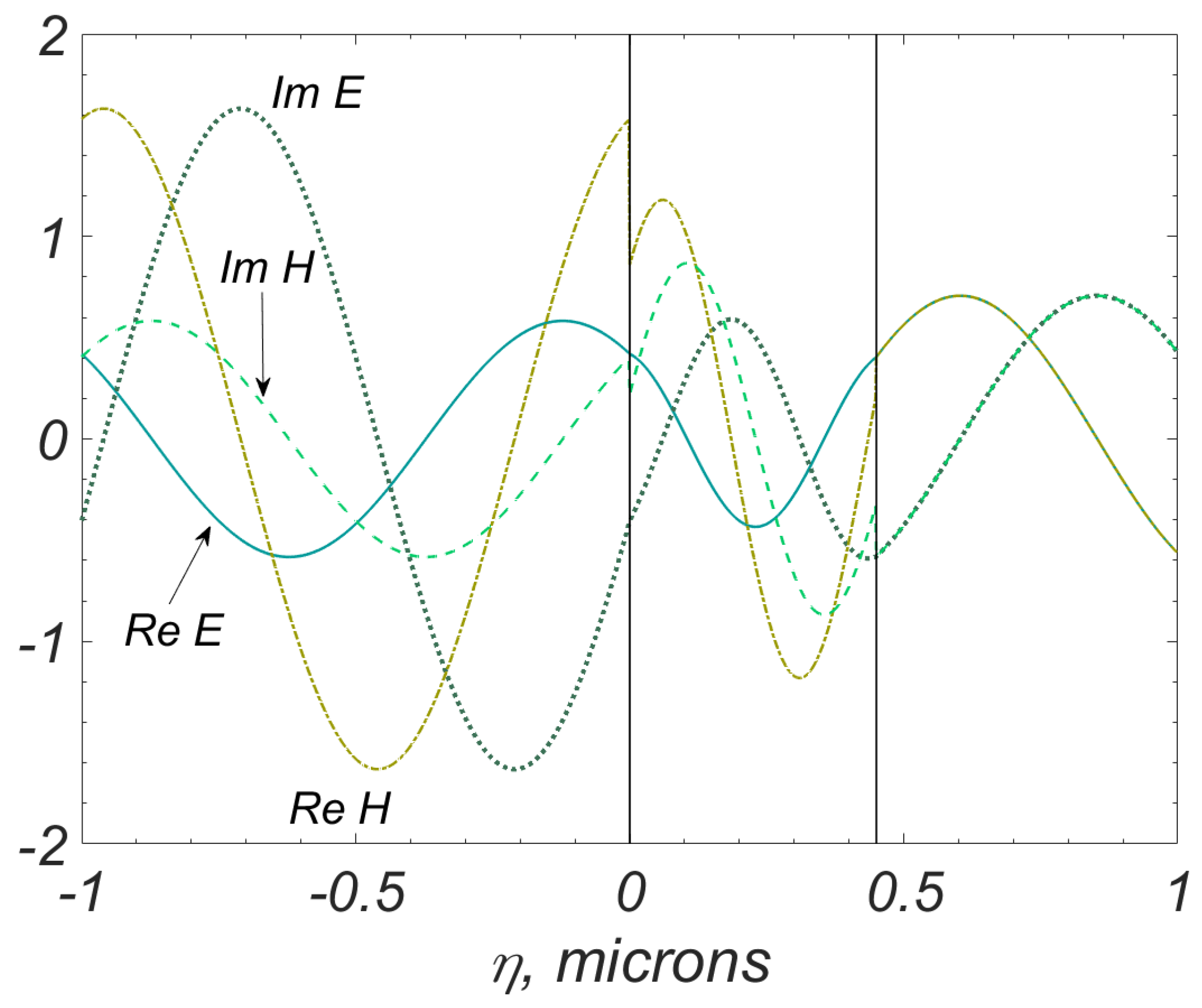
3. Finally, let us compare the bicompact scheme and the classical finite element and finite difference methods for solving a one-dimensional problem along the ray coordinate. As already noted, the amplitudes of the fields undergo a strong discontinuity at the interface of the media. For example, for the s-polarization, the field amplitude H experiences a discontinuity (see Figure 3), and the field E is continuous. The magnitude of the gap is subject to the conjugation conditions. In [44], comparative testing of bicompact scheme and classical methods of finite differences in the time domain and finite elements on problems with strong discontinuities of the solution was carried out. It showed that in this case, the error of classical methods does not decrease with decreasing grid step; i.e., there is no convergence.

The reason for this is as follows. The convergence of classical schemes is proved for sufficiently smooth solutions. It is well known [45] that in order to calculate problems with generalized solutions, it is necessary to use completely conservative schemes, which are the grid implementation of all the necessary conservation laws. For the problem under consideration, the physical conservation laws are the integral Maxwell equations. The interface conditions at the interface of media are their consequence. Classical difference methods do not take into account boundary conditions in the case of strong discontinuities. At the same time, bicompact scheme accounts for these conditions explicitly and confidently copes with such tasks.

5. Method Validation

In the two following sections, the verification of the optical path method and bicompact scheme is carried out. In these problems, we consider the media to be spatially homogeneous, and the incident field to be monochromatic. Note that the scope of applicability of the proposed approaches is much wider: they are applicable if the media are spatially heterogeneous, and the incident radiation can be non-monochromatic. However, for piecewise homogeneous media, using matrix methods, it is possible to calculate the exact values of the reflectance R and transmittance T. Possessing the exact solution, one can perform a thorough verification of the proposed methods. Therefore, we chose this particular case as a test. Nevertheless, it is quite representative.

We emphasize that the transition from a stationary formulation to a non-stationary one is reduced to a direct and inverse Fourier transform. This approach is reliably verified in [12]. Therefore, calculations of non-stationary problems are not carried out in this work.

6. Fabry–Perot Interferometer

Consider the oblique incidence of a plane wave on a plane-parallel plate (the Fabry–Perot interferometer). Let the plate thickness be d and the interface boundaries correspond to the planes $z=b$ and $z=b+d$. The plate is located in the air.

6.1. Transparent Plate

1. Let the material parameters of the plate be $\epsilon =4$, $\mu =1$, and the thickness is $d=0.5$ microns. The refractive index is real; i.e., the plate is optically transparent. The wavelengths $\lambda \in (0.5,3)$ microns are considered: from the middle of the visible range to the upper limit of the short infrared range. We select the angle $\alpha$ so that $cos\beta$ is a rational number. This permits us to eliminate the influence of round-off errors when calculating trigonometric functions and check convergence more accurately. Let us put $cos\beta =9/10$. Then, $\alpha =\arcsin (\sqrt{\epsilon }cos\beta )\approx 1.059\approx 60.{67}^{°}$. The zeros in the reflection spectrum correspond to the phase incursion $\delta =2\pi m$, $m=1,2,\dots$, see the formula (23). The corresponding wavelengths are equal to

$$\lambda =2cos\beta /m=9/\left(5m\right),\mathrm{microns}m=1,2,\dots .$$

(39)

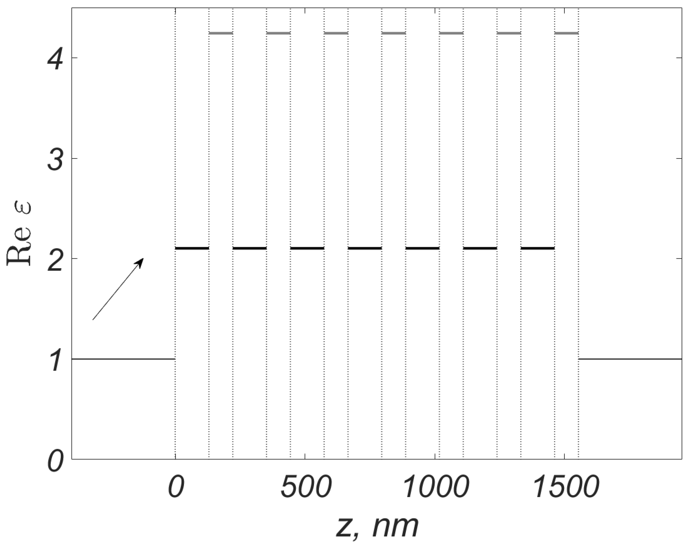
2. Figure 3 shows the complex amplitudes of the fields depending on the ray coordinate in the case of s-polarization. Vertical lines are the layer boundaries. One can see that $\mathrm{Re}E$ and $\mathrm{Im}E$ are continuous, and $\mathrm{Re}H$ and $\mathrm{Im}H$ experience a discontinuity at both boundaries. This is consistent with the conjugation condition (27).

Figure 3. Fabry–Perot interferometer, s-polarization. Complex amplitudes of fields depending on the ray coordinate. Vertical lines are layer boundaries.

Figure 3. Fabry–Perot interferometer, s-polarization. Complex amplitudes of fields depending on the ray coordinate. Vertical lines are layer boundaries.

3. Let us note one nuance. For practice, it is not only the value of R or T in some characteristic region of the spectrum (for example, in the local minimum or local maximum of reflection) that matters but also the position $\lambda$ of this characteristic region. This is due to the fact that in typical photonics problems, the spectra of $R\left(\lambda \right)$ and $T\left(\lambda \right)$ have areas of sharp change (large gradients). Therefore, a small horizontal shift of the spectrum leads to a significant change in R and T at a fixed $\lambda$.

Therefore, to estimate the proximity of the spectral curves, we choose not classical norm of their difference but the Hausdorff metric [46]. Recall its definition. Let U and V be two nonempty compact subsets of the metric space M. Let these sets consist of points $\mathbf{u}$ and $\mathbf{v}$, respectively. Then, the distance from U to V is

$$\delta (U,V)=max\{\underset{\mathbf{v}\in V}{sup}\underset{\mathbf{u}\in U}{inf}|\mathbf{u}-\mathbf{v}|,\underset{\mathbf{u}\in U}{sup}\underset{\mathbf{v}\in V}{inf}|\mathbf{u}-\mathbf{v}|\}$$

(40)

Due to taking the operation sup, the definition (40) resembles the C norm. If in this definition, we replace sup with an integral over $d\lambda$, take $|\mathbf{u}-\mathbf{v}|$ squared and take the square root from the answer, then the resulting metric resembles the $L_2$ norm.

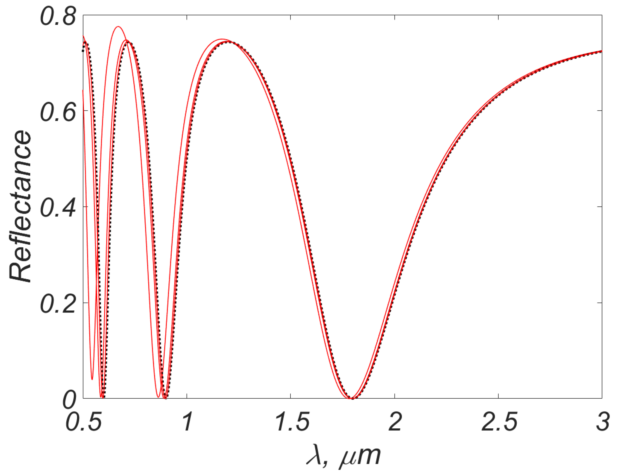
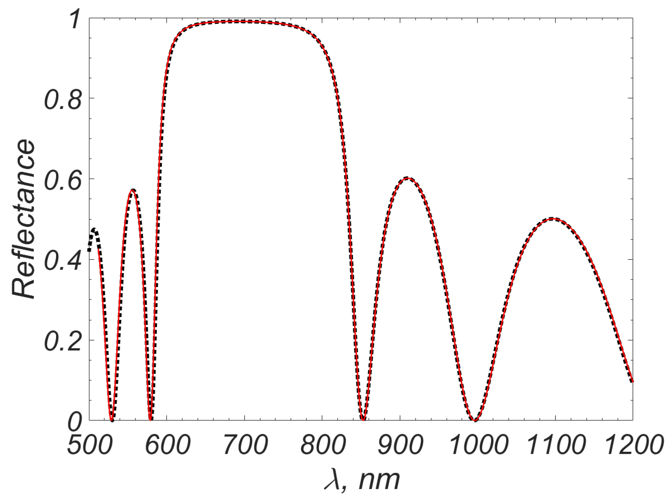
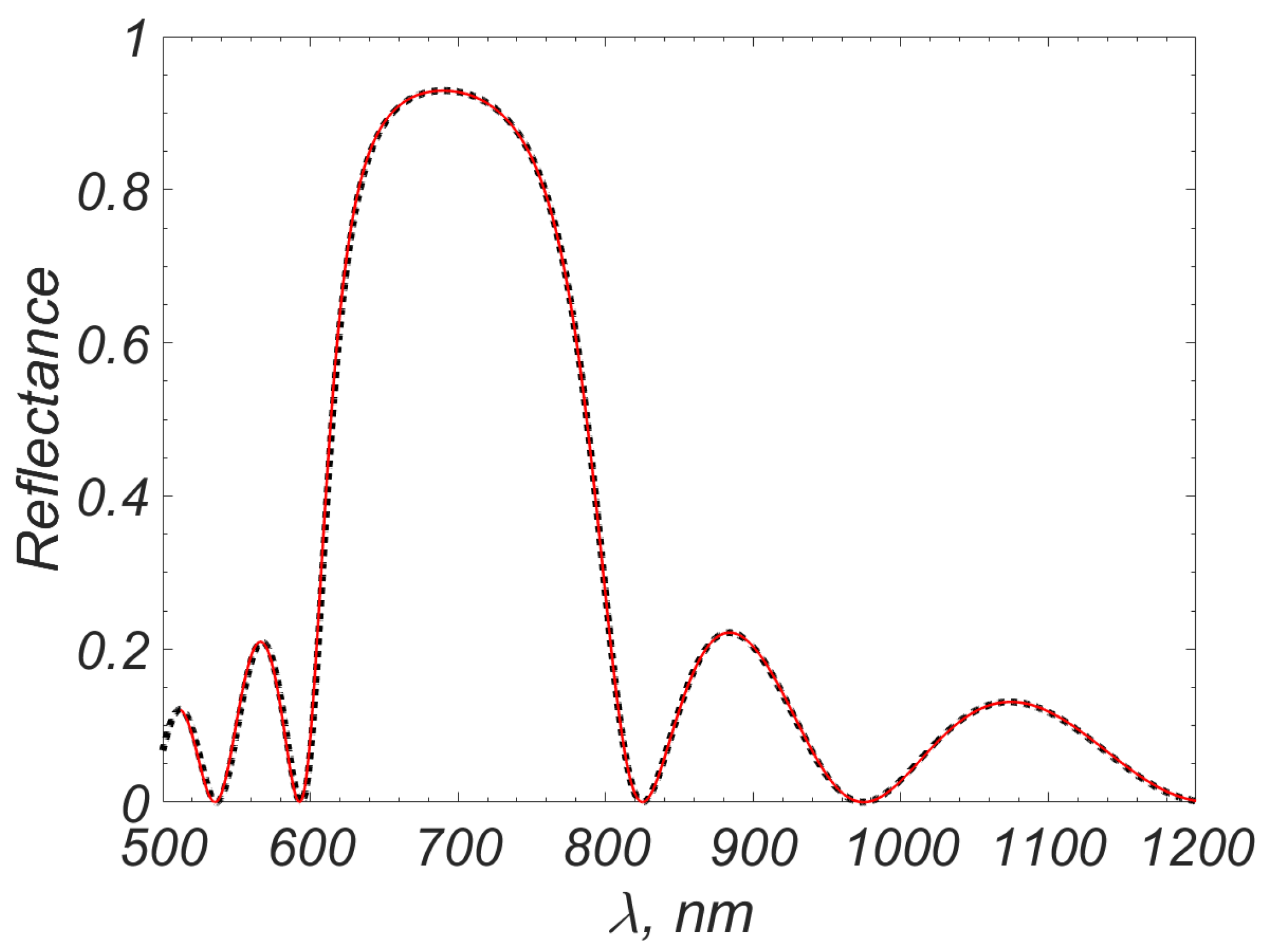
4. Figure 4 shows the dependence of the reflection coefficient R on the wavelength $\lambda$. The dotted line is the exact spectrum found by the matrix method. Solid lines are calculations using the optical path method and a bicompact scheme corresponding to several thickening grids in space. From grid to grid, the number of steps is doubled and the length of the steps decreases by the factor of 2. One can see that as the grids thicken, the profiles $R\left(\lambda \right)$ tend to the limit that corresponds to the exact spectrum. This tendency has the character of horizontal shift. This type of convergence confirms the reasonability of choosing the Hausdorff metric for comparing the calculated curves.

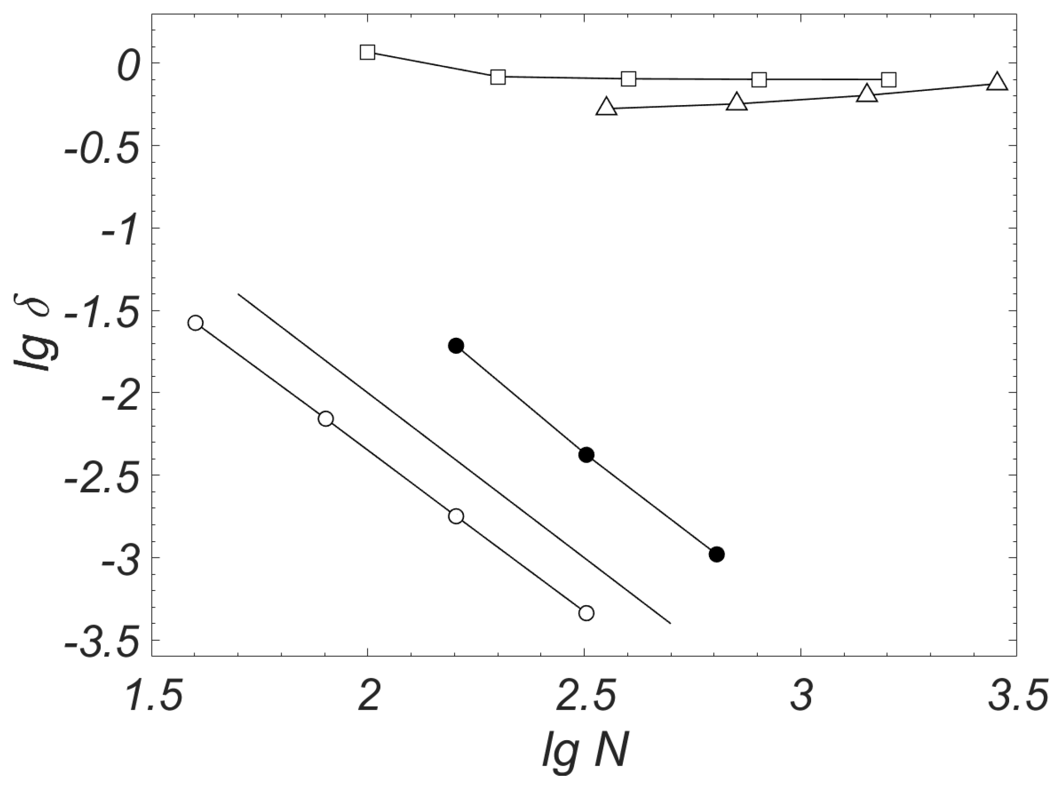
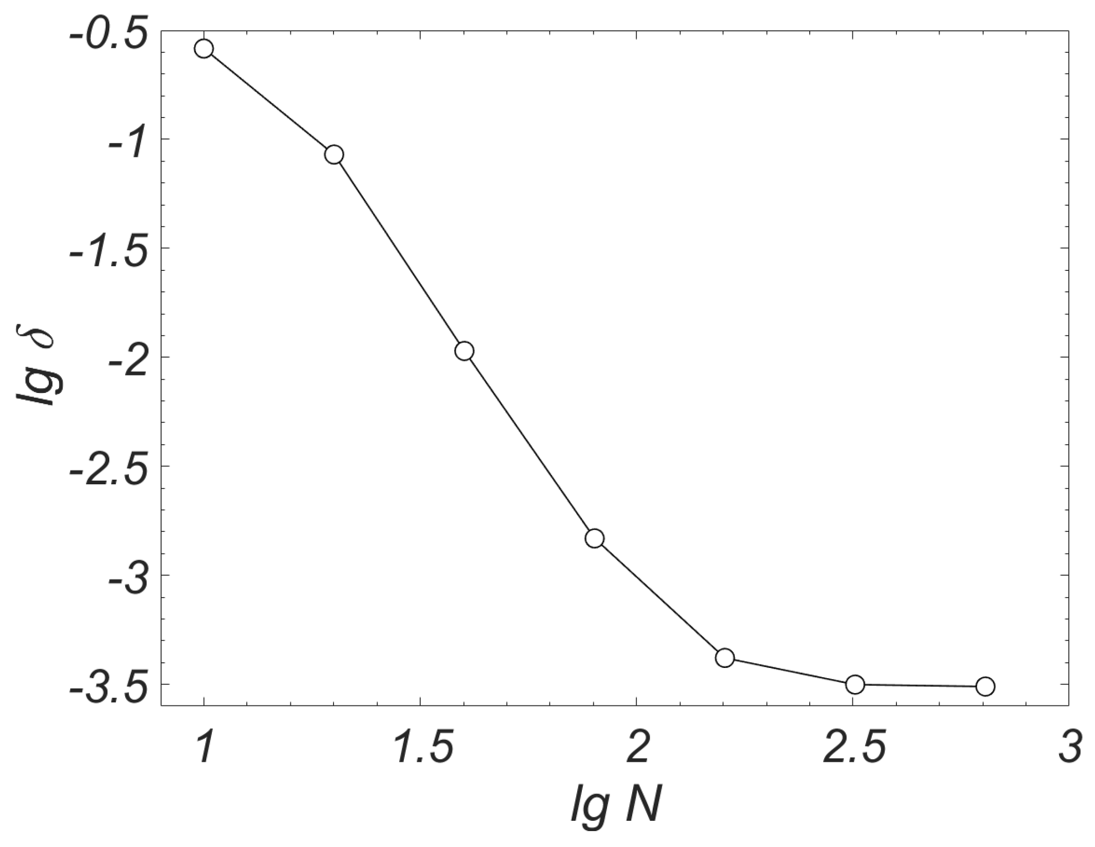
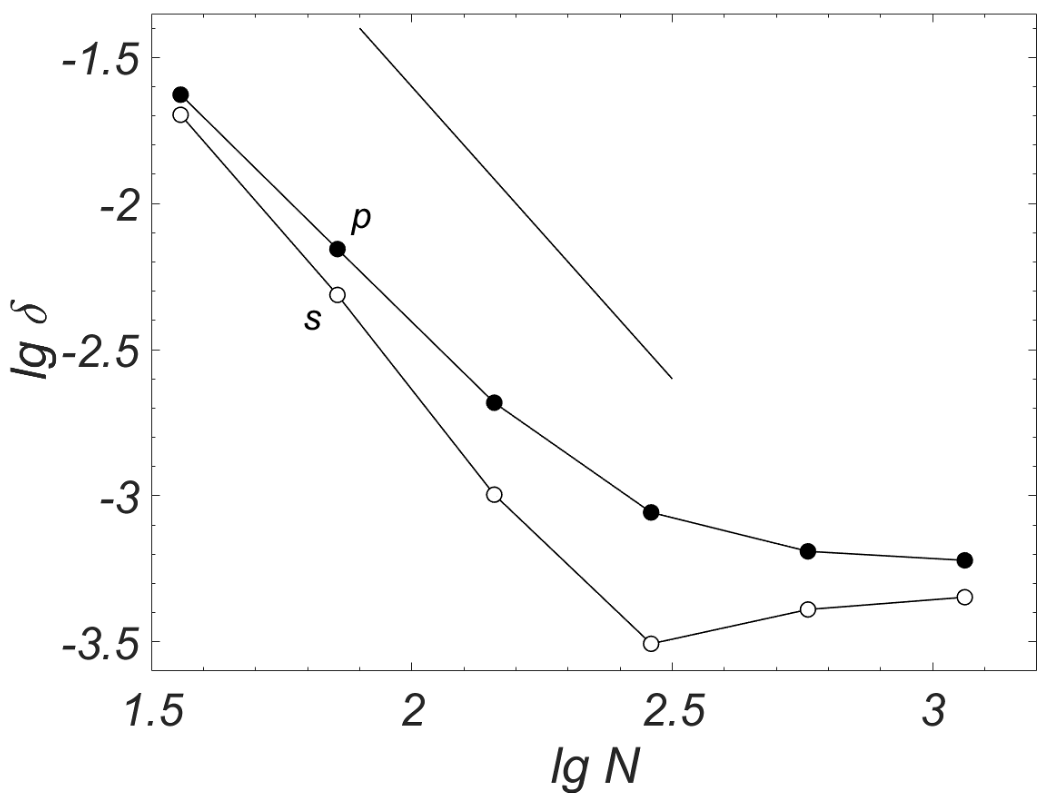
5. Figure 5 shows the error of the spectra calculated by the proposed methods for the case of s-polarization. The error was calculated as the distance between the calculated spectrum and the exact spectrum found using the matrix method in the Hausdorff metric. The graph is given in double logarithmic scale; the power convergence corresponds to a straight line with a slope equal to $-p$, where p is the order of accuracy.

It can be seen that the curve tends to a straight line, the slope of which is $-2$. This means that when the spatial grids thicken, the error decreases, and the rate of its decrease is $O\left(h^2\right)$, which corresponds to the second order of accuracy of the finite-difference scheme. At the same time, the proposed scheme provides high quantitative accuracy: already on the grid with $N=80$ steps, the error is $\sim 1$%. This is enough for practical applications.

Similar results were obtained for the case of p-polarization. The corresponding errors are also shown in Figure 5.

6. For comparison, calculations of the problem along the optical beam were carried out using classical schemes: the finite element method in the frequency domain (FEFD) and finite difference method in the time domain (FDTD). Recall that these methods do not take into account the conjugation conditions (21) and (22). The errors obtained in the calculation for s-polarization are shown in Figure 5. It can be seen that for both schemes, the error does not decrease with the thickening of the grid, i.e., there is no convergence. This shows the importance of taking into account physically correct interface conditions at the interface boundaries.

6.2. Lossy Plate

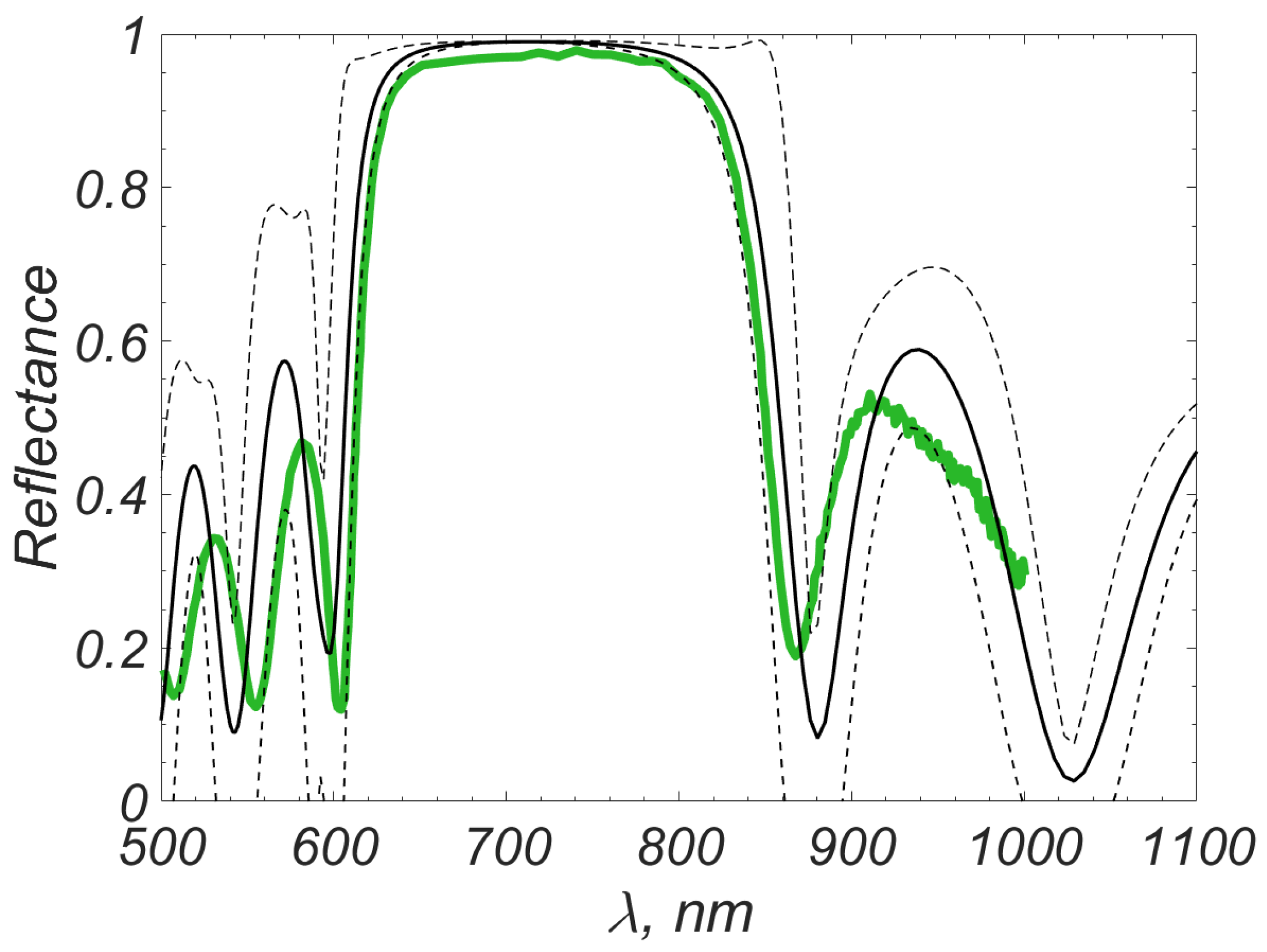
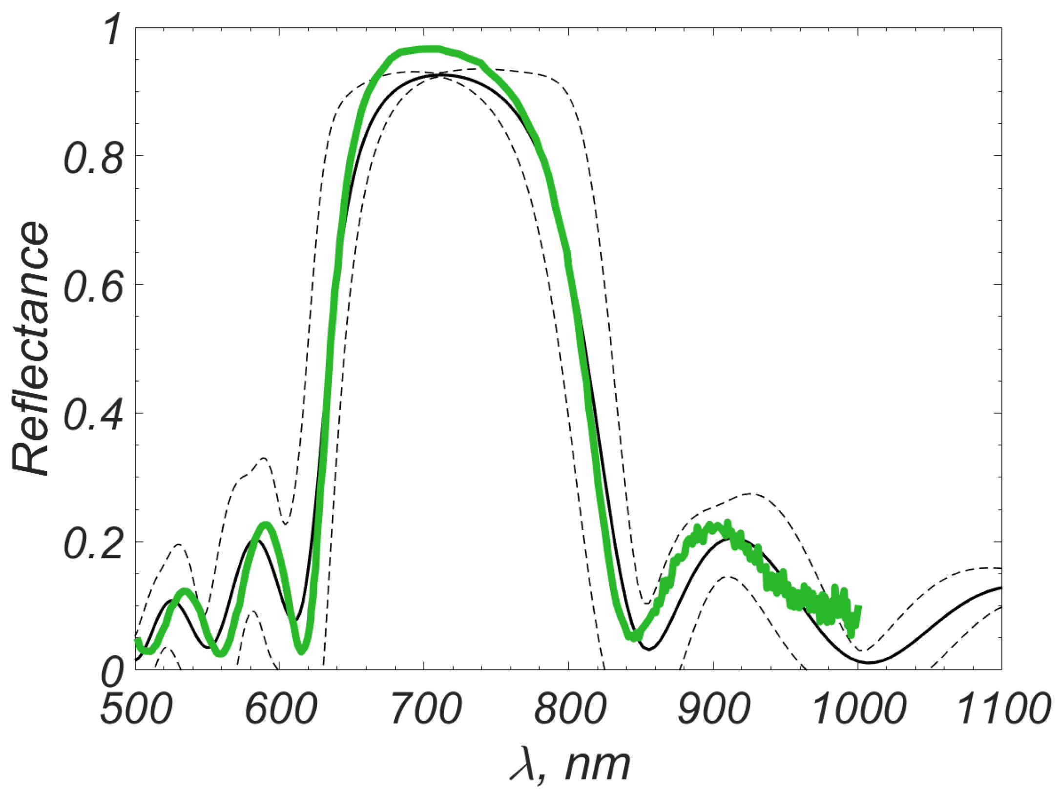
Now let the plate be metal with $\epsilon =-120+3i$. This value corresponds, for example, to the dielectric constant of silver at a wavelength of 1.5 microns. The considered wavelengths lie in the range $\lambda \in (0.5,12)$ microns; its lower boundary is the middle of the visible range, and the upper one is the end of the second transparency window for thermal imaging.

The calculated reflection spectra for s-polarization are shown in Figure 6. It can be seen that as the meshes thicken, the spectrum found using the optical path method and the bicompact scheme tends to a certain limit function (i.e., there is convergence of the difference scheme). However, this limit function differs from the exact spectrum found using the matrix method. The reason for the discrepancy is a physical error introduced by the optical path method in an absorption medium.

Figure 7 shows the errors in the calculation using the optical path method and the bicompact scheme versus the number of grid steps. The graph is plotted in double logarithmic scale. It can be seen that on coarse grids, the error decreases at a rate approximately corresponding to $O\left(h^2\right)$. Thereby, the grid error of the difference scheme is decisive on these grids. On sufficiently detailed grids, the error reaches the value of $\sim 0.3$% and stops decreasing. This means that the determining contribution is not the grid error but the physical error. Recall that it is irremovable. However, this accuracy is quite sufficient for physical applications.

Calculations for p-polarization gave the same result. The corresponding error curve almost coincides with Figure 7.

7. Spectra of Photonic Crystals

7.1. Structure

Consider a photonic crystal (PC) consisting of 7 pairs of layers {SiO₂—130 nm, Ta${}_2$O${}_5$—92 nm} [3]. This structure is shown in Figure 8. A plane linearly polarized monochromatic wave falls on the structure from $z=-\infty$. The angle of incidence is 45^o.

The dependence of the dielectric permittivity of these materials on the wavelength is shown in Figure 9. Experimental reflection spectra of this PC at the angle of incidence $\alpha ={45}^{°}$ for s- and p-polarizations are published in [3].

7.2. Calculated Spectra

1. For the s-polarized wave, the reflection spectrum is shown in Figure 10. The band-gap is clearly visible in the wavelength range of $600\sim 850$ nm; in this range, the PC is a mirror for a given angle of incidence. To the left and right of the band-gap, reflection minima are visible, which correspond to almost complete passage.

For a p-polarized wave, the reflection spectrum is shown in Figure 11. The band-gap corresponding to the wavelengths of $600\sim 800$ nm is visible, and there is almost zero reflection minima to the left and right of it.

In Figure 12, the errors of the spectra for both polarizations calculated using the proposed approaches are shown. As before, the error refers to the distance between the calculated spectrum and the exact one (found using the scattering matrix method) in the Hausdorff metric. The scale of the graph is double logarithmic.

It can be seen that for both polarizations, the errors decrease in accordance with the second order of accuracy up to a value of 0.1%. Furthermore, the errors stop decreasing and come out on horizontal lines. The reason for this is that the physical approximations of the optical path method described in Section 4.5 introduce some error that does not decrease with decreasing grid step. Nevertheless, it can be seen that this error is small, and the physical accuracy of the optical path method is obviously sufficient for practical tasks.

7.3. Experimental Spectra

1. The manufacture of optical nanostructures is a complex technological process. Because of this, the geometric parameters of the scatterer (for example, the thickness of the PC layers) may fluctuate. These fluctuations are several percent of the size of the scatterer. They introduce significant distortions in the electromagnetic response of the structure [10].

Therefore, fluctuations in the thickness of the PC layers affect the interference of reflected waves inside the PC. The presence of a systematic error in the thicknesses leads to a shift of the minima in the reflection spectrum. Random errors lead to a blurring of the minima and their rise above the abscissa axis.

2. To take into account thickness fluctuations, we apply the virtual experiment method we proposed earlier [12]. Recall the essence of this approach.

Let one of the parameters of the problem A be known with the error ${\sigma }_A$. We assume this parameter to be a normally distributed random variable with a mathematical expectation of A and a standard deviation of ${\sigma }_A$. The electromagnetic response of the structure is a function of this random variable. Therefore, the calculation results must be averaged over the distribution of the value A. At the same time, one can find the confidence interval of the averaged calculation, i.e., the error estimate introduced by the error of setting the value A.

3. In [3] and other works of this team, we have not found fluctuation estimations of the layer thicknesses of the PC under consideration. Therefore, we selected the statistical characteristics of these fluctuations so that the averaged calculated spectrum best described the experimental spectrum. We introduce a systematic error $h_0$ of thicknesses, which for simplicity we assume to be the same for all layers. We also introduce a random error, which is distributed according to the Gauss law with zero mean and standard deviation ${\sigma }_0$. Realizations of random error may be different for different layers.

The value of $h_0$ was selected by the position of the reflection minima, and the standard ${\sigma }_0$ was chosen to describe their depths. For both polarizations, the values of $h_0\approx 3$ nm, ${\sigma }_0\approx 3.5$ nm turned out to be practically optimal.

4. Comparison of the obtained averaged spectrum with the experimental one is shown in Figure 13 (for s-polarization) and Figure 14 (for p-polarization). Additionally, confidence intervals of the averaged spectrum equal to two standard deviations are shown.

It can be seen that the positions of the extremums in the calculated and experimental spectra coincide with an accuracy of 1–2%. This accuracy can be considered excellent. The reflection values themselves concide with an accuracy of mostly 1–4%; occasionally, the error increases to $\sim 10$%. This corresponds to the typical accuracy of experimental measurements. Almost the entire experimental curve lies inside the confidence corridor around the calculated curve. This confirms the reasonability of the selected ${\sigma }_0$ and $h_0$.

5. Therefore, the calculations of this section show that the optical path method is applicable to a wide range of important applied tasks.