On the Control over the Distribution of Ticks Based on the Extensions of the KISS Model

Abstract

Ticks and tick-borne diseases present a well-known threat to the health of people in many parts of the globe. The scientific literature devoted both to field observations and to modeling the propagation of ticks continues to grow. To date, the majority of the mathematical studies have been devoted to models based on ordinary differential equations, where spatial variability was taken into account by a discrete parameter. Only a few papers use spatially nontrivial diffusion models, and they are devoted mostly to spatially homogeneous equilibria. Here we develop diffusion models for the propagation of ticks stressing spatial heterogeneity. This allows us to assess the sizes of control zones that can be created (using various available techniques) to produce a patchy territory, on which ticks will be eventually eradicated. Using averaged parameters taken from various field observations we apply our theoretical results to the concrete cases of the lone star ticks of North America and of the taiga ticks of Russia. From the mathematical point of view, we give criteria for global stability of the vanishing solution to certain spatially heterogeneous birth and death processes with diffusion.

1. Introduction

Ticks and tick-borne diseases present a well-known threat to the health of people in many parts of the globe. The scientific literature devoted both to field observations and to modeling the propagation of ticks continues to grow.

To date, the majority of the mathematical studies were devoted to models based on ordinary differential equations, where spatial variability was taken into account by a discrete parameter. One of the most basic models was developed in [1], which is an ODE in four parameters (number of ticks V, number of hosts N, number of infected ticks X, number of infected hosts Y), and where the standard quadratic term of logistic models (expressing the internal competition of species) was replaced by a term limiting the growth of ticks by the number of available hosts. Apart from the analysis of equilibria (and their stability) performed for this model, Gaff et al. [1] also suggested a variant with multiple patches (with some fixed rates of transmission between them), however, with only a numerical analysis for this advanced variant.

In White et al. [2], this model was further developed to include the dynamics of two pathogens. Very complicated extensions (with various variables and parameters) were suggested and analyzed in [3,4,5]. In [6], a fractional version of tick-host dynamics was developed.

A stochastic version (Markov-chain model) of the model [1] was developed in [7], and the extinction predictions for deterministic and stochastic models were compared. In Gaff et al. [8] the models from a previous work [1] were enhanced by introducing some control parameters and the related optimal control policies (for quadratic costs) were derived aimed at reducing the propagation of diseases.

In two other studies [9,10], models with delays were suggested and analyzed via various methods (Lyapunov functions, Hopf bifurcations). A cellular-automaton model for the spatial propagation of ticks was developed and analyzed numerically in [11].

In Mwambi et al. [12], a stage-structured population model was proposed and analyzed. In the present paper we extend partially this model by including spatial dynamics.

Tosato et al. [13] investigated how different types of host targeted tick-control strategies (combined acaricide-repellent control) affect tick population and disease transmission, leading to some remarkable counterintuitive conclusions.

A reaction-diffusion model for the propagation of lyme disease was suggested [14] extending a similar spatially trivial model [15]. In a paper by Caraco et al. [14], the dynamics involved 9 density-variables: susceptible mice M, infected mice m, questing larvae L, larvae infesting susceptible mice V, larvae infesting pathogen infected mice v, susceptible questing nymphs N, questing infectious nymphs n, uninfected adult ticks A, pathogen infected adult ticks a. Position-independent equilibria were obtained and their local stability was investigated. This model was further developed by Zhao et al. [16], where the global stability of spatially trivial equilibria was analyzed for the case of bounded domains and the travel wave solutions were constructed for the case of unbounded domains.

The exploitation of partial differential equations for the analysis of spatial distribution of various species is a standard tool in ecology [17,18]. The latter paper, in particular, discussed the advantages and disadvantages of using the standard diffusion models, as compared with the models based on the telegraph equation. Recent references include papers [19,20] that deal with an attraction-repulsion chemotaxis model.

One of the standard tools is the so-called KISS model (from Kierstead, Slobodkin and Skellam, see [21,22]). It was developed initially in the framework of the plankton propagation. It describes the minimal size of a patch, where the population can survive under killing (mathematically Dirichlet) conditions on the boundary. For instance, in a one-dimensional case we look at the equation $\dot{y}=a{y}^{″}+\lambda y$, with $a,\lambda >0$ (see (1) below for all notations), on an interval $[0,R]$ with the conditions $y\left(0\right)=y\left(R\right)=0$. The minimal R, for which a solution will not necessarily tend to zero, as time goes to infinity, is referred to as the critical patch size or the KISS scale. More generally one considers the behavior of the population when the interval $[0,R]$ is surrounded by an infinite non-beneficial territory, where the dynamics are described by the equation $\dot{y}=a{y}^{″}-\mu y$, with $\mu >0$. The critical size then decreases depending on the ratio $\lambda /\mu$. A review of these results and their various extensions can be found in [23], see also [24].

Let us mention a very important development of the KISS model for the description of several interacting species (though less relevant to the present paper), in particular diffusive versions of the Lotka–Volterra equations, which dealt with patchiness (spatially nontrivial stationary solutions) and its stability, see, e.g., [25,26,27].

The KISS model is the starting point for our analysis. However, eventually we are interested in creating control zones (kind of barriers) with non-beneficial conditions that can stop the propagation of ticks. We first extend the KISS model to the case when the non-beneficial region is bounded, interpreting its size as an additional control parameter, and the diffusion coefficient is discontinuous at the interface of beneficial and non-beneficial regions together with the mortality coefficient. Then we consider the modifications of the model with various boundary conditions, most importantly with the periodic boundary conditions. Seemingly not very relevant from the practical point of view, they provide the key intermediate step to tackle our main questions: how to organize the sizes and properties of the regular patches of (intermittent) control zones that would prevent the growth of the population of ticks. Our main results are partial answers to this question. We give first rather precise results for a homogeneous population, and then extend them partially to the structured populations, with several stages, such as larvae, nymphs, and adult ticks.

We suppose that in the control zone one is able to achieve the required level of the death rates or to decrease the reproduction rates of ticks. In the literature, one can find various methods that can be used locally for this purpose. It can be achieved by the treatment of the soil (planned burns, cleaning and decreasing humidity levels, chemical treatment, see, e.g., [13,28] and references therein), by tick-targeted strategies such as TickBots (see, e.g., [13,29]), by specific actions on hosts, such as dipping of cattle with acaricide (see, e.g., [30,31]) or by biological methods such as infesting woods with ants (see [32] for the related experiments on ants in the USA and [33] for the experiments in Russia), or natural enemies of ticks, such as the insects Ixodiphagus hookeri (see, e.g., [28]).

From the mathematical point of view, what we are doing here is obtaining criteria for negativity of certain differential operators, or more precisely, looking for the precise estimates to their highest eigenvalue. This is one of the basic problems in the theory of pseudo-differential equations. Many general results are available, which are often given; however, for the operators with smooth (at least major) symbol and/or up to certain constants, see, e.g., [34,35]. Here we solve this problem for a class of second order operators with piecewise continuous symbols. The negativity of the diffusion operators that govern the propagation of ticks ensures that the population will eventually die out (in the region considered).

The content of the paper is as follows. In Section 2, our models are introduced, and the main mathematical results are formulated. The first introductory subsection deals with a simple scalar model of one-dimensional diffusion. We give the necessary and sufficient conditions for the negativity of the corresponding diffusion operators (that imply the eradication of ticks) with various boundary conditions under the additional complication of discontinuous diffusion coefficients. These results should be of no surprise to specialists (they might be even known, but the author did not find a proper reference), because they are related to the famous Kronig-Penney model (though there the diffusion coefficient is a constant) of quantum mechanics. These results are tailored in a way to be used for concrete calculations on ticks given below.

The main results are obtained further. They concern the case of vector-valued diffusions, which allows one to analyse the evolution of the densities of ticks on various stages of their development. We first suggest some general, though rather rough, sufficient conditions for negativity by the method of symmetrization. Then we give some more precise conditions, but only in the case of two-stage populations and under rather restrictive assumptions on the control parameters.

In Section 3, we apply our theoretical results to the two examples of tick populations, the lone star tick, Amblyoma Americanum, from the south of USA, and the taiga tick, Ixodes persulcatus, the major type in Russian Siberian forests. There exist quite a lot of field investigations devoted to these species and thus an abundance of the observations, see, e.g., [30,36] and references therein for the American ticks and [28,37] for the taiga tick. Much less information is available for the European tick, Ixodes ricinus. However, as was previously noted in the mathematical modeling literature (see, e.g., [1]), there is no consensus on many parameters required for modelling, and the available parameters are varying by the types of the territories (upper or bottom land, upland wooded, meadow, etc), humidity and temperature, seasonal oscillation of hosts, etc. Therefore, numeric estimates of the parameters are obtained by applying some reasonable averages from the parameters found in the literature. Section 4 presents the graphs of certain simulations illustrating the decay of ticks’ populations under numeric data of the previous section. Section 5 is devoted to the proofs of our results. In the last section, some conclusions are drawn and further perspectives are indicated.

2. Models and Theoretical Results

2.1. Warm-Up: One-Stage Modeling

In this paper, we address the following question: can one place some barriers, organized by some control zones that are not beneficially for the multiplication of ticks, which would practically stop their propagation beyond these control zones?

Since we are talking about spatial propagation, our model must be necessarily spatially nontrivial. Therefore, we shall apply a diffusion model. As was mentioned above, a diffusion model was developed by Caraco et al. [14]. Unlike the model of this paper, our model here will be simpler, in the sense that we will stick to linear modeling (unlike the reaction-diffusion setting of [14]), but, on the other hand, it will include additional complication of being spatially heterogeneous, and precisely the effective control of these heterogeneities will be the main objective.

Remark 1. 

By not including in the model the quadratic (logistic type) terms of the standard nonlinear model, we are not including the competition between species, thus allowing ticks to multiply and propagate under better conditions than for nonlinear models. Consequently, if we manage to achieve the decay of their propagation in our linear case (what we are doing here), then the same decay will hold as well for the corresponding models with additional nonlinear terms limiting their growth. Moreover, since we are effectively giving stability criteria for the vanishing solution of a linear equation in a strong asymptotic sense (all eigenvalues have negative real part), adding additional quadratic terms can neither spoil this stability, nor improve it. The latter means that if there exists a mode with a positive eigenvalue of the linear part, then the vanishing solution will not be stable even in the presence of quadratic terms. This justifies the use of the linear model for our purposes in general term. Finally, the competition in ticks is performed mostly via available spaces on the bodies of hosts, so that the quadratic term in the equations for the dynamics of ticks is proportional to $V(MN-V)$ (see [1]), with the number of ticks V, the number of hosts N, and the maximum number M of ticks per host. Therefore, when hosts are in abundance, as compared to the basic equilibrium concentration of ticks (for instance, this occurs in many areas of Siberian taiga, see [28,37]), quadratic terms can be considered as overall negligible as compared to linear terms.

In order to not overcomplicate the story, we will not distinguish between infected and noninfected ticks, aiming at their total eradication (at least locally) and we shall not include explicitly the dynamics of hosts (mice, deer, etc.), their overall influence being reflected just by specifying certain average speed of motion of ticks, which will be effectively modeled as the diffusion coefficient. Moreover, though the natural state space for the dynamics of ticks is two-dimensional, we shall stick here to a one-dimensional modeling having in mind the propagation in a certain direction, with the second coordinate averaged out.

The ticks are known to have several stages in their development (larvae, nymphs, adult). To better explain our ideas, we shall first consider the model, where all generations are averaged out, and next describe the modifications arising when several distinct generations are explicitly included in the model.

Thus, we start with the simplest diffusion model for the dynamic of ticks in some area of their habitat (we denote the derivatives with respect to time and space by a dot and a prime, respectively):

$$\dot{y}=a{y}^{″}+\lambda y,y(0,x)=y_0\left(x\right).$$

(1)

Here $a>0$ is a diffusion coefficient reflecting the average speed of their random wandering and the coefficient $\lambda >0$ reflects the speed of their multiplication (usually represented as the difference of average birth rates and average mortality). The density $y=y(t,x)$ on some interval $x\in [0,R]$ evolves according to (1) subject to additional boundary conditions, which can be taken as the Dirichlet conditions ($y(t,0)=y(t,R)=0$), or as the Neumann conditions ($y^{\prime }(t,0)=y^{\prime }(t,R)=0$) (or more general mixing Robin conditions that we shall not touch here), or rather periodic conditions ($y(t,0)=y(t,R)$, $y^{\prime }(t,0)=y^{\prime }(t,R)=0$).

Remark 2. 

The Dirichlet conditions arise in the situation, when ticks cannot survive at the boundary, which can be given, for instance, as a water reservoir, or as a temperature barrier. The Neumann conditions arise in the situation with reflecting barrier, such as a natural or artificial hedge. In other words, this is the situation, when no flux of matter crosses the border of the system either from outside or from inside. Periodic conditions do not seem to have a natural interpretation, but they are often convenient for the analysis (and therefore are abundantly used in physics), and can be also used as an intermediate step. In particular, the Dirichlet conditions are clearly the most disastrous for ticks, and therefore, if one can prove the dying out of ticks for periodic conditions, then the same will hold for the Dirichlet conditions. It is also intuitively clear (and again widely used in physics) that for large intervals the difference in boundary conditions does not affect the solutions in any essential way.

The main point in our modeling is the possibility to attach to the main region $[0,R]$ (the background or the beneficial zone) a control zone of (much smaller length) r, which is not beneficial for ticks, meaning that their reproduction coefficient becomes negative there. One may also be able to control the diffusion coefficient shifting it to a different value b. Thus, instead of a homogeneous model (1) we consider a model with two distinctive regions:

$$\begin{array}{cc}\hfill & {\dot{y}}_{ben}=a{y}_{ben}^{″}+\lambda y_{ben},x\in (0,R)\hfill \\ \hfill & {\dot{y}}_{nb}=b{y}_{nb}^{″}-\mu y_{nb},x\in (R,R+r),\hfill \end{array}$$

(2)

where positive $\mu ,b,r$ are our control parameters. Here $y_{ben}$ stands for the background beneficial region for ticks, which is not under our control, and $y_{nb}$ stands for the small non-beneficial region, where we are supposed to have control over at least some parameters. To make the problem well posed we should add, as above, some boundary conditions for $x=0$ and $x=R+r$ and moreover, the standard gluing conditions for diffusions with discontinuous coefficients (see, e.g., [38]):

$$y_{ben}\left(R\right)=y_{nb}\left(R\right),a{y}_{ben}^{\prime }\left(R\right)=b{y}_{nb}^{\prime }\left(R\right).$$

(3)

Let the operator L be defined on the functions of the interval $[0,R+r]$ by the formula

$$Ly\left(x\right)=\left\{\begin{array}{c}a{y}_{ben}^{″}\left(x\right)+\lambda y_{ben}\left(x\right),x\in (0,R)\hfill \\ b{y}_{nb}^{″}\left(x\right)-\mu y_{nb}\left(x\right),x\in (R,R+r).\hfill \end{array}\right.$$

(4)

It is a standard fact from the theory of diffusion operators that, restricted to the functions satisfying the gluing condition (3) and either Dirichlet, or Neumann or periodic conditions, the operator L becomes self-adjoint with a discrete spectrum in the Hilbert space of the square integrable functions $L_2\left([0,R+r]\right)$ on $[0,R+r]$. Moreover, this operator is bounded from above, so that there exist a decreasing sequence of eigenvalues $l_0\ge l_1\ge l_2\ge \cdots$ and the corresponding orthonormal basis $\{{\xi }_j\}$ in $L_2\left([0,R+r]\right)$ (depending on the chosen boundary conditions) such that $L{\xi }_j=l_j{\xi }_j$ for all j. This implies that for any initial function $y_0$ from $L_2\left([0,R+r]\right)$ the solution to (2) with this initial condition is given by the convergent series

$$y\left(x\right)=\sum _j{e}^{t{l}_j}{\xi }_j\left(x\right){\int }_0^{R+r}{y}_0\left(z\right){\xi }_j\left(z\right)dz.$$

Consequently, if all $l_j$ are negative, i.e., the operator L is negative, then this solution tends to zero for any initial conditions. Thus, the condition of eventual eradication of ticks in our model is the condition of negativity of L, or equivalently, the condition of the absence of nonnegative eigenvalues. In the rare case of vanishing maximal eigenvalues, the solution converges to a finite limit as $t\to \infty$.

Theorem 1. 

Assume the Dirichlet boundary conditions. (i) If

$$\lambda /a\ge {\pi }^2/R^2,$$

(5)

L has a positive eigenvalue (independently of $\mu ,r$!).

(ii) If

$${\pi }^2/{\left(2R\right)}^2<\lambda /a<{\pi }^2/R^2,$$

the operator L is negative if and only if

$$-\frac{tanh\left(r\sqrt{\mu /b}\right)}{\sqrt{b\mu }}>\frac{tan\left(R\sqrt{\lambda /a}\right)}{\sqrt{a\lambda }}.$$

(6)

(iii) If

$$\lambda /a\le {\pi }^2/{\left(2R\right)}^2,$$

L has no nonnegative eigenvalues (and is negative in the case of the strict inequality).

Statement (i) is the well-known (initial) result of the KISS model yielding the critical patch size

$$R_c=\pi \sqrt{a/\lambda },$$

see [21,22]. Statement (ii) was proved for the limit $r\to \infty$ in [22].

Evidently, for the Neumann and periodic boundary condition the situation is different. There is no critical size, as the population can survive on any small interval. However, as the following results show, by introducing appropriate control zones, one can eradicate the population in a similar way to the above.

Theorem 2. 

Assume the Neumann boundary conditions. (i) If

$$\lambda /a\ge {\pi }^2/{\left(2R\right)}^2,$$

L has a positive eigenvalue (independently of $\mu ,r$!).

(ii) Otherwise, L is negative if and only if

$$\sqrt{\mu b}tanh\left(r\sqrt{\mu /b}\right)>\sqrt{\lambda a}tan\left(R\sqrt{\lambda /a}\right),$$

(7)

so that one can achieve negativity by choosing appropriate μ and r.

Theorem 3. 

Assume the periodic boundary conditions. (i) If (5) holds, then L has a positive eigenvalue. (ii) Otherwise, L is negative if and only if

$$\sqrt{\mu b}tanh\left(\frac{r}{2}\sqrt{\mu /b}\right)>\sqrt{\lambda a}tan\left(\frac{R}{2}\sqrt{\lambda /a}\right).$$

(8)

One sees that Theorem 3 provides the same condition as Theorem 2 though with $R/2$ and $r/2$ instead of R and r. On the other hand, the boundary KISS value of (5) is the same for the Dirichlet and the periodic conditions. Moreover, one can check explicitly from conditions (8) and (6) that, as expected (see Remark 2), if the operator L is negative under the periodic condition, then it is also negative under the Dirichlet conditions.

Theorems 1 and 3 provide exact information on how $\mu ,b,r$ can be tuned in order to achieve negativity of L and hence the eventual eradication of ticks. We see, in particular, that if R does not exceed certain critical level, one can eradicate the ticks by introducing a control zone of arbitrary small length r, if a sufficiently high level of mortality $\mu$ can be imposed on this control zone.

On the other hand, the theorems show that if $\lambda R^2/a$ is large enough, then no control zone can efficiently influence the global growth of the tick population. This observation leads to a natural idea that, in the case of a large territory, one can fight with the growth of ticks by arranging several small control zones placed in a periodic (patched) fashion. As we are going to show, if this is organized in a way that each pair of adjacent zones satisfies the conditions of the previous theorem, the ticks will be eradicated in the whole patched territory.

Thus, assume that our territory of habitat is represented as the interval $[0,K(R+r\left)\right]$, with some natural K, and that it is decomposed into $2K$ subintervals, odd $I_1=[0,R]$, $I_3=[R+r,2R+r]$, ⋯, $I_{2K-1}=[(K-1)(R+r),KR+(K-1)r]$, so that $I_{2k-1}=[(k-1)(R+r),kR+(k-1)r]$ for $k=1,\cdots ,K$, and even $I_2=[R,R+r],\cdots ,I_{2K}=[KR+(K-1)r,K(R+r)]$, so that $I_{2k}=[kR+(k-1)r,k(R+r)]$ for $k=1,\cdots ,K$. Assume that on the long odd intervals we have some background parameters $\lambda >0,a>0$, and on the short even intervals we have some (controllable) parameters $b>0,\mu >0$, so that the diffusion is given by the first and second equations of (4) on even and odd intervals, respectively; see Figure 1.

Evidently, the gluing conditions (3) are supposed to hold on the interface of all intervals. Theorem 3 (valid for the case $K=1$) can now be extended to the case of arbitrary K as follows.

Theorem 4. 

Assume the periodic boundary conditions for such diffusion on $[0,K(R+r\left)\right]$. Then for any K the conditions of Theorem 3 provide also the conditions for the corresponding diffusion operator L on $[0,K(R+r\left)\right]$ to be negative or not.

Remark 3. 

As we already mentioned, if all positive solutions for the periodic conditions tend to zero, as $t\to \infty$, then the same holds for the Dirichlet conditions. It is intuitively clear, as the Dirichlet conditions are less beneficial for survival. Formally it follows from the representations of solutions in terms of the Feynmann–Kac formula.

2.2. Several-Stage Modeling: Trivial Case

Until now, we have considered the situation with all stages of ticks’ lives averaged out. In more precise modeling, one has to take into account the presence of several stages. For ticks these are eggs, larvae, nymphs, and adults. With some reasonable averaging one can reduce the consideration of the lifespan of ticks to the two basic periods, from eggs to nymphs, and from nymphs to hatching female adults. On the other hand, a more detail analysis, can include not only the stages, but their time developments. Namely, say, nymphs can develop to adults in the same season as their own molting takes place, or after a diapause (wintering), so one can distinguish not only the stage, but also whether it develops in one year or two years.

Let us consider the general case of n stages (could be also generations for other species). The basic Equation (1) is generalized to the vector-valued equation

$$\dot{y}=a{y}^{″}+My,y(0,x)=y_0\left(x\right),$$

(9)

where $y\in {\mathbf{R}}^n$ and M is the birth-and-death matrix showing the progression of ticks from their birth through their various stages of development. This matrix $M=M_n$ has the standard form (used by many authors, see, e.g., [12] or [16]) reflecting the sequential propagation through various stages. They have elements

$$M_{jj}=-m_j,j=1,\cdots ,n,M_{j+1,j}=b_j,j=1,\cdots ,n-1,M_{1n}=b_n,$$

(10)

with all other elements vanishing, where all parameters $m_j$ and $b_j$ are positive.

For instance, for dimensions 2 and 3, these matrixes have the form

$$M_2=\left(\begin{array}{c}-m_1{b}_2\hfill \\ b_1-m_2\hfill \end{array}\right),M_3=\left(\begin{array}{c}-m_{1}0b_3\hfill \\ b_1-m_{2}0\hfill \\ 0b_2-m_3\hfill \end{array}\right).$$

(11)

It is easy to see that a matrix M of type (10) always has a real eigenvalue.

Let us assume now that we can set a control zone with the increased death rates for ticks. Namely, let us consider the extension of Equation (2) of the form

$$\begin{array}{cc}\hfill & {\dot{y}}_{ben}=a{y}_{ben}^{″}+M{y}_{ben},x\in (0,R)\hfill \\ \hfill & {\dot{y}}_{nb}=b{y}_{nb}^{″}+(M-\mu \mathbf{1})y_{nb},x\in (R,R+r),\hfill \end{array}$$

(12)

where $\mathbf{1}$ is the unit matrix. Notice that $\mu$ here has a slightly different meaning as in (2), referring to the relative decrease in the death rates. The corresponding diffusion operator becomes matrix-valued:

$$Ly\left(x\right)=[a{y}^{″}\left(x\right)+My\left(x\right)]{\mathbf{1}}_{[0,R]}\left(x\right)+[b{y}^{″}\left(x\right)+(M-\mu \mathbf{1})]{\mathbf{1}}_{[R,R+r]}\left(x\right).$$

It turns out that the results of Theorems 1–4 have a straightforward extension to this case with the role of $\lambda$ played by the largest eigenvalue of M.

Theorem 5. 

Assume that the maximal real eigenvalue ${\mathrm{\Lambda }}_1$ of the matrix M in (12) is positive (if all eigenvalues of M have negative real parts, then the population would die out even in the background territory, the case of no interest to us) and all other eigenvalues ${\mathrm{\Lambda }}_j$ have negative real part and are different (the latter conditions are technical simplifications that are not essential). Assume also that $\mu >{\mathrm{\Lambda }}_1$ (otherwise the ticks could survive even in the control zone alone).

Assume the Dirichlet boundary conditions for L. (i) If

$${\mathrm{\Lambda }}_1/a\ge {\pi }^2/R^2,$$

(13)

L has a positive eigenvalue. (ii) If

$${\pi }^2/{\left(2R\right)}^2<{\mathrm{\Lambda }}_1/a<{\pi }^2/R^2,$$

(14)

the operator L is negative if and only if

$$-\frac{tanh\left(r\sqrt{(\mu -{\mathrm{\Lambda }}_1)/b}\right)}{\sqrt{b(\mu -{\mathrm{\Lambda }}_1)}}>\frac{tan\left(R\sqrt{{\mathrm{\Lambda }}_1/a}\right)}{\sqrt{a{\mathrm{\Lambda }}_1}}.$$

(15)

(iii) If

$${\mathrm{\Lambda }}_1/a\le {\pi }^2/{\left(2R\right)}^2,$$

(16)

L has no nonnegative eigenvalues (and is negative in the case of the strict inequality).

Assume now that the territory of habitat is represented by the interval $[0,K(R+r\left)\right]$ (with some natural K), decomposed into $2K$ subintervals in the same way as formulated before Theorem 4, and that on the odd and even intervals our diffusion follows the first and the second equation of (12), respectively, with the usual gluing condition on the interfaces.

Theorem 6. 

Let the conditions of Theorem 5 for M hold and K be arbitrary. Assume that the periodic boundary conditions are chosen. (i) If (13) holds, then L has a positive eigenvalue. (ii) Otherwise the operator L is negative if and only if

$$\sqrt{(\mu -{\mathrm{\Lambda }}_1)b}tanh\left(\frac{r}{2}\sqrt{(\mu -{\mathrm{\Lambda }}_1)/b}\right)>\sqrt{{\mathrm{\Lambda }}_{1}a}tan\left(\frac{R}{2}\sqrt{{\mathrm{\Lambda }}_1/a}\right).$$

(17)

2.3. Several-Stage Modeling: Advanced Case

This section contains our main theoretical results.

Until now, we have looked at the case when diffusion coefficients differ in beneficial and control zones, but are independent of the stage. Evidently, usual averaging allows one to apply this model for ticks. However, for many types of ticks, larvae and nymphs use small rodents as hosts, while adult ticks use large mammals, such as deer, or birds, so that the displacement, and hence the diffusion coefficient differs drastically for the adults and the earlier stages of ticks. Hence it is more natural to use the model with different diffusions on different stages. Moreover, the matrixes M specifying the birth and death rates, can be of course quite different for the background and control zones, thus differing not only by a multiple of the unit matrix, as in (12).

Let us start with a simple extension of the KISS model. Namely, let us consider the extension of Equation (9) with variable diffusion, i.e., the equation

$$\dot{y}=A{y}^{″}+My,y(0,x)=y_0\left(x\right),$$

(18)

where A is a diagonal matrix with diagonal elements $a_j>0$, $j=1,\cdots ,n$.

Theorem 7. 

Let M be a matrix of type (10). Suppose that the maximal eigenvalue ${\mathrm{\Lambda }}_1=\mathrm{\Lambda }(M,A)$ of the matrix $A^{-1}M$ is strictly positive. Then the critical patch size equals $R_c=\pi /\sqrt{{\mathrm{\Lambda }}_1}$. That is, there exists a nontrivial solution to the equation $A{y}^{″}+My=Ey$ with the Dirichlet boundary conditions and with some positive E if and only if $R>R_c$.

The story becomes more complicated when we put together the original and a control zones. It seems difficult to expect here explicit necessary and sufficient conditions for the negativity of the spectrum, such as in the cases analyzed above. However, reasonable sufficient conditions can be obtained, as we are going to show now.

Let us consider the system

$$\begin{array}{cc}\hfill & {\dot{y}}_{ben}=A_{ben}{y}_{ben}^{″}+M_{ben}{y}_{ben},y\in (-R/2,R/2),\hfill \\ \hfill & {\dot{y}}_{nb}=A_{nb}{y}_{nb}^{″}+M_{nb}{y}_{nb},y\in (R/2,r+R/2),\hfill \end{array}$$

(19)

with symmetric positive matrixes $A_{ben}$, $A_{nb}$ and arbitrary matrixes $M_{ben}$, $M_{nb}$, where matrixes $M_{nb}$, $A_{nb}$ are supposed to depend on some control parameters. We assume the periodic boundary conditions and the usual gluing conditions ($y_{nb}=y_{ben}$, $A_{nb}{y}_{nb}^{\prime }=A_{ben}{y}_{ben}^{\prime }$) on the interface.

Equations for the eigenvalues are

$$\begin{array}{cc}\hfill & A_{ben}{y}_{ben}^{″}+M_{ben}{y}_{ben}=E{y}_{ben}\hfill \\ \hfill & A_{nb}{y}_{nb}^{″}+M_{nb}{y}_{nb}=E{y}_{nb}.\hfill \end{array}$$

(20)

Theorem 8. 

Assume exactly k out of n eigenvalues ${\lambda }_1\ge \cdots \ge {\lambda }_n$ of the symmetric matrix $N_{ben}=(M_{ben}{A}_{ben}^{-1}+A_{ben}^{-1}{M}_{ben}^T)/2$ are positive, and all eigenvalues ${\mu }_1\ge \cdots \ge {\mu }_n$ of the symmetric matrix $N_{nb}=(M_{nb}{A}_{nb}^{-1}+A_{nb}^{-1}{M}_{nb}^T)/2$ are negative (by T we denote the transposition). If

$$R\le R_c^{sym}=\pi /\sqrt{{\lambda }_1},$$

(21)

and

$$\frac{\sqrt{|{\mu }_1|}sinh\left(r\sqrt{|{\mu }_1|}\right)}{1+cosh\left(r\sqrt{|{\mu }_1|}\right)}>\frac{2Rnk{\lambda }_1}{1+cos\left(R\sqrt{{\lambda }_1}\right))},$$

(22)

then system (20) has no solutions with non-negative E (and periodic boundary conditions).

This result extends automatically to the case of the territory represented by the interval $[0,K(R+r\left)\right]$, with some natural K, which is decomposed into $2K$ subintervals in the same way as formulated before Theorem 4 (see also Theorem 6), so that on the odd and even intervals the diffusion follows the first and the second equation of (19).

Notice that the l.h.s. of (22) increases as $\sqrt{|{\mu }_1|}$ as in our previous results, but the r.h.s. is of order ${\lambda }_1$ (for R far away from $R_c^{sym}$), unlike $\sqrt{{\lambda }_1}$ in Theorem 3.

In Theorem 7, the condition of the existence of a positive eigenvalue is given in terms of the maximal eigenvalue ${\mathrm{\Lambda }}_1$ of the matrix $A^{-1}M$ and in Theorem 8 a sufficient condition for negativity is linked with the maximal eigenvalue of the corresponding symmetrized matrix. Hence from the combination of these two theorems nothing can be said for sizes R such that

$$\pi /\sqrt{{\lambda }_1}=R_c^{sym}<R<R_c=\pi /\sqrt{{\mathrm{\Lambda }}_1}.$$

(23)

In order to work with these sizes, the effective method of symmetrization used in Theorem 8 cannot be applied, and the analysis in arbitrary dimension seems to be quite involved. Working in dimension $n=2$, where explicit formulas for eigenvectors allow for a rather detailed analysis, possible results seem to depend strongly on the structure of diffusion coefficients and the matrix M. We present one such result valid for a range of coefficients that can be applied to tick populations.

Let us look at the equations

$$\begin{array}{cc}\hfill & {\dot{y}}_{ben}=A{y}_{ben}^{″}+M_{ben}{y}_{ben}\hfill \\ \hfill & {\dot{y}}_{nb}=aA{y}_{nb}^{″}+M_{nb}{y}_{nb}\hfill \end{array}$$

(24)

and the corresponding eigenvalue problem

$$\begin{array}{cc}\hfill & A{y}_{ben}^{″}+M_{ben}{y}_{ben}=E{y}_{ben}\hfill \\ \hfill & aA{y}_{nb}^{″}+M_{nb}{y}_{nb}=E{y}_{nb},\hfill \end{array}$$

(25)

with the usual gluing condition: $y_{ben}$ coincides with $y_{nb}$ and $y_{ben}^{\prime }$ coincides with $a{y}_{nb}^{\prime }$ on the interface of two regions.

Let $n=2$. For a $E\ge 0$, denote by ${\mathrm{\Lambda }}_1\left(E\right)\ge {\mathrm{\Lambda }}_2\left(E\right)$ the eigenvalues of the matrix $N_{ben}\left(E\right)=A^{-1}{M}_{ben}-A^{-1}E$, and by ${\mu }_1\left(E\right)\ge {\mu }_2\left(E\right)$ the eigenvalues of the matrix $N_{nb}\left(E\right)=(A^{-1}{M}_{nb}-A^{-1}E)/a$. Let ${\mathrm{\Lambda }}_1={\mathrm{\Lambda }}_1\left(0\right)>0>{\mathrm{\Lambda }}_2\left(0\right)$ and $E_0>0$ be such that ${\mathrm{\Lambda }}_1\left(E_0\right)=0$. Assume that ${\mathrm{\Lambda }}_1\left(E\right)\ge 0>{\mathrm{\Lambda }}_2\left(E\right)$ and $0>{\mu }_1\left(E\right)>{\mu }_2\left(E\right)$ for all $E\in [0,E_0]$. Let $\{v_j\left(E\right)\}$ and $\{w_j\left(E\right)\}$ be the corresponding bases of eigenvectors of $N_{ben}\left(E\right)$ and $N_{nb}\left(E\right)$, and $c\left(E\right)=\left(c_{ij}\left(E\right)\right)$ be the matrix that takes the basis $\{v_j\left(E\right)\}$ to the basis $\{w_j\left(E\right)\}$.

Theorem 9. 

Assume the bases of eigenvectors can be chosen in such a way that

$$c_{12}\left(E\right)c_{21}\left(E\right)\le 0,c_{11}\left(E\right)c_{22}\left(E\right)\ge 0$$

(26)

for $E\in [0,E_0]$. Then, if

$$a\sqrt{|{\mu }_1\left(0\right)|}tanh\left(\sqrt{|{\mu }_1\left(0\right)|}\frac{r}{2}\right)>\sqrt{{\mathrm{\Lambda }}_1}tan\left(\sqrt{{\mathrm{\Lambda }}_1}\frac{R}{2}\right),$$

(27)

there are no solutions to Equation (25) with periodic boundary conditions and non-negative E.

Comparing (27) with (8) we see that under (26) our two-dimensional condition of negativity is the exact extension of the one-dimensional case.

Remark 4. 

The technically convenient assumptions (26) (and especially the first of these two) are not very natural and should not hold in a general situation. However, as we show below, they can be achieved by an appropriate proportional change of the elements of the birth-and-death matrix.

Let us now look at a concrete situation when (26) holds. Namely, consider the system (24) where $a=1$, the matrix A is diagonal with the diagonal elements $a_1,a_2$ $M_{ben}$ has the form $M_2$ from (11) and $M_{nb}$ has the same form with ${\tilde{m}}_j$ and ${\tilde{b}}_j$ instead of $m_j$ and $b_j$. Thus

$$N_{ben}\left(0\right)=A^{-1}{M}_{ben}=\left(\begin{array}{c}-a_1^{-1}{m}_1{a}_1^{-1}{b}_2\hfill \\ a_2^{-1}{b}_1-a_2^{-1}{m}_2\hfill \end{array}\right),N_{nb}\left(0\right)=A^{-1}{M}_{nb}=\left(\begin{array}{cc}& -a_1^{-1}{\tilde{m}}_1{a}_1^{-1}{\tilde{b}}_2\hfill \\ & a_2^{-1}{\tilde{b}}_1-a_2^{-1}{\tilde{m}}_2\hfill \end{array}\right).$$

Assume that we can control the non-beneficial zone by a proportional decrease of the reproduction coefficients, i.e., calibrating

$${\tilde{b}}_j=\omega b_j,j=1,2,$$

(28)

by choosing an appropriate parameter $\omega \in (0,1)$ and choosing ${\tilde{m}}_j\ge m_j$ in such a way that

$${\tilde{m}}_1-{\tilde{m}}_2\ge m_1-m_2.$$

(29)

For real ticks, $a_1$ is usually much less than $a_2$ (see numeric examples below). Hence the assumptions of the next theorem are fully relevant.

Theorem 10. 

Assume that $det{N}_{ben}\left(0\right)=m_1{m}_2-b_1{b}_2<0$ (this enures that ${\mathrm{\Lambda }}_1\left(0\right)>0>{\mathrm{\Lambda }}_2\left(0\right)$) and

$$a_1^{-1}\ge a_2^{-1},a_1^{-1}{m}_1\ge a_2^{-1}{m}_2.$$

(30)

Assume that ${\tilde{b}}_j$ and ${\tilde{m}}_j$ satisfy (28) and (29). Then the conditions of Theorem 9 (namely, inequalities (26)) hold, so that (27) is sufficient for the absence of nonnegative eigenvalues.

3. Numerical Results with Real Life Data

3.1. One-Stage Modeling with the North American Ticks

In US, the predominant types of ticks are the lone star tick (Amblyoma Americanum) in the south, the blacklegged tick (Ixodes scapularis, formerly called the deer tick) and the Americal dog tick (Dermacenter Variabilis) in the north. One can find lots of experimental research on the various parameters needed for modeling, which depend on many factors. Here, to estimate the birth and death rates, we will employ the averaged parameters for the lone star tick from [1]. Namely, the time unit is a month. Taking 2000 as the average number of eggs (occurring once in two year), $70\%$ survival rate and sex ratio 1:1, we obtain the birth rate of female larvae per month to be $0.5\times 0.7\times 2000/24$. With the out of host survival average 0.85 and the probability to find the host 0.03 (recall that without finding a host for a full meal blood no further development of a tick is possible) the total survival rate (of females) per month is calculated in [1] as

$$0.5\times 0.7\times 2000/24\times 0.03\times 0.85=0.75.$$

Death rate is estimated as $0.01$ in woods and as $0.1$ in grass. Sticking to the case of grass, we obtain the parameter $\lambda$ in Equation (1) to be $\lambda =0.75-0.1=0.65$ (measured in month⁻¹).

To estimate the diffusion coefficient a is a more difficult task.

We shall use the standard method, used both in physics and ecology (see, e.g., [17]), where the mean squared displacement $M^2\left(t\right)$ during a time t is estimated as

$$M^2\left(t\right)=2at.$$

(31)

The lifetime of the majority of lone star ticks is known to be 2 years, but sometimes it is over in one year. Thus, we can assume approximately that it has two rides per year. The main hosts for the lone star ticks (and many other American Ticks) are the white tailed deer that could travel for many kilometers during the 3–4 days needed for a tick to obtain its blood meal. One can choose about 10 km as the reasonable estimate for an average distance per a ride (see [31]). Note that the displacement due to ticks’ own movement is negligibly small compared to their displacement by the hosts.

Then the total squared displacement is $M^2\left(12\right)={(2\times 10)}^2=400$, and therefore a = 400:24 ≈ 16.67, measured in km² per month. Thus, for the critical patch size we obtain

$$R_c=\pi \sqrt{16.67/0.65}\approx 15.9\left(\mathrm{km}\right).$$

(32)

Theorems 1–4 can be used to define the exact relation between the length of a control zones and the death rate in it, which is needed for the eradication of ticks.

For instance, let us apply Theorem 4.

Let us choose $R=14$ (km) (which is reasonably close to the critical size $R_c$) and the length of the control zone $r=1$ (km), and let $b=a$ for simplicity. Then condition (8) for the eradication of ticks obtains the following numeric form

$$\sqrt{16.67\mu }tanh\left(0.5\sqrt{\mu /16.67}\right)>17.03,$$

(33)

so that the minimal required death rate $\mu$ is rather high, about 1960. These numbers are summarized in Figure 2.

3.2. One-Stage Modeling with the Taiga Ticks

Let us exploit here another time unit, choosing it to be one year. The life cycle of the taiga tick varies from 3 to 6, so that four years can be taken as an approximate average. Recall that in order to have a molting and to turn from one stage to another (larvae to a nymph, nymph to an adult, and finally to hatch) a tick must have a ride on a host with a full meal. Hence with 3–4 year cycle a tick makes on average a single ride per year.

Taking, as above, 10 km as an average distance per a meal (and thus per year) we obtain from (31) that $a=100/2=50$, measured in km² per year.

As the mean survival rate we choose $\lambda =2$, measured in year⁻¹, which is the approximate value used in [11], where it was shown to produce a reasonable fit to the experimental data available. Thus, for the critical patch size we obtain

$$R_c=\pi \sqrt{50/2}\approx 15.7\left(\mathrm{km}\right),$$

(34)

giving approximately the same result (!), as in the calculations above, based on the American experimental data.

3.3. Two-Stage Modeling with the Taiga Ticks

One of the ways to estimate the average travel distance of ticks on hosts can be obtained using chemical treatments of a controlled territory and looking for how far ticks can penetrate into the treated territory from the uncontrolled zone. These studies indicate (see Section VIII.3 of [28]) that, for a taiga tick, one can choose about 10 km as the average displacement for adult ticks during their meals (supporting the number used above and taken from the literature on American ticks) and about 1.5 km for nymphs and larvae. Therefore the diffusion coefficient $a=100/2=50$, used above for the whole population of ticks, in a more detailed analysis becomes the diffusion coefficient $a_2=50$ for the adult ticks only, while for all lower stages it can be estimated as only $a_1=1.5^2/2\approx 1.1$.

Let us work with the two-stage model, where the first stage represents the species grown up to the well-fed nymph, and the second stage represents adults. We shall use here the data for the taiga tick from the Sayans mountains of Siberia, Krasnoyarsk region, as presented in the very detailed observations of [37]. These observations show that only about $2.4\%$ of female tick obtain their meal and that about $1/2$ of well-fed females produce eggs in the amount of about 5 thousand each. Taking also the standard sex ratio as 1:1, it follows that the potential number for the next generation is

$$p=5000\times 0.024\times 0.5^2=30$$

per an adult tick. From this amount about $43\%$ survive producing hungry nymphs in the amount of $0.43p=12.9$. Only $8.2\%$ of the potential p survive to the stage of an adult well-fed nymphs (because of the high death rate on this stage), i.e., in total remain $0.082p=2.46$ per an original adult tick.

Next, the death rate from a well-fed nymph to an adult tick is about $14.6\%$, and the death rate during a winter is about $39\%$. Thus, from a well-fed nymph one can expect about

$$0.854\times 0.61\approx 0.52$$

hungry adults to appear next spring. Thus, the birth-and-death matrix M and the diffusion matrix A in (18) take the concrete form

$$M=\left(\begin{array}{c}-12.46\hfill \\ 0.52-1\hfill \end{array}\right),A=\left(\begin{array}{c}1.10\hfill \\ 050\hfill \end{array}\right).$$

(35)

Therefore

$$A^{-1}M=\left(\begin{array}{c}-0.912.46\times 0.91\hfill \\ 0.52\times 0.02-0.02\hfill \end{array}\right)=\left(\begin{array}{c}-0.912.24\hfill \\ 0.01-0.02\hfill \end{array}\right).$$

For the positive eigenvalue ${\mathrm{\Lambda }}_1$ of this matrix we obtain approximately $\sqrt{{\mathrm{\Lambda }}_1}=0.067$ and thus the critical patch size of Theorem 7 equals

$$R_c=\pi /0.067\approx 46.9.$$

(36)

This value is essentially larger than the values (32) and (34), calculated for one-stage models and data (and taken from different sources). This can be expected. In fact, more detailed observations and calculations based on the regions of approximate equilibrium should reflect only slight possible average growth rates and hence weaker requirements for control zones. Theorem 10 can be used to assess the required decrease in the reproduction rates of control zones that would ensure the eradication.

Choosing, say, $R=40,r=1$, the condition of negativity (27) obtains the following numeric form:

$$\sqrt{{\mu }_1\left(0\right)}tanh(\sqrt{{\mu }_1\left(0\right)}/2)>0.067tan\left(1.34\right)=0.29.$$

(37)

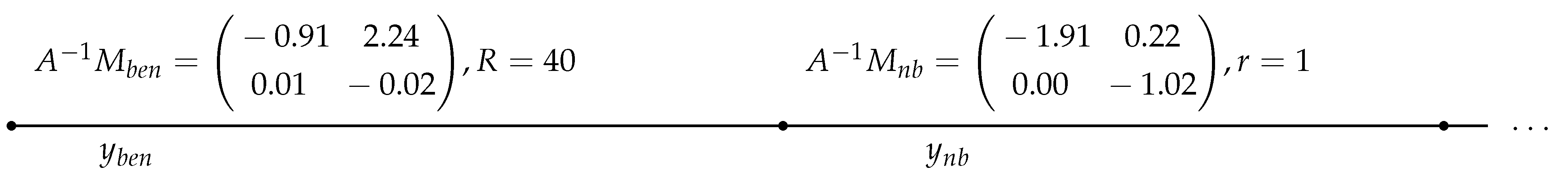
Therefore $|{\mu }_1|$ must be larger than about $0.64$. This condition yields the corresponding estimates for the required ${\tilde{m}}_j,{\tilde{b}}_j$. This setting is given schematically on Figure 3.

On the other hand,

$$\frac{1}{2}(A^{-1}M+M^T{A}^{-1})=\left(\begin{array}{c}-0.911.125\hfill \\ 1.125-0.02\hfill \end{array}\right).$$

Consequently, one obtains for the highest eigenvalue ${\lambda }_1$ of this symmetrized matrix that ${\sqrt{\lambda }}_1\approx 0.86$. Therefore

$$R_c^{sym}=\pi /0.863\approx 3.64.$$

(38)

This value is much less than values (32) and (34). This corroborates the idea that the results of Theorem 8, which are very natural, theoretically, must be used cautiously in situations with highly nonsymmetric birth-and-death matrixes, as the symmetrization leads to strong distortions for such data.

Remark 5. 

One of the ways to enhance the practical application of Theorem 8 might be the introduction of additional life stages (increasing dimension) that would make the birth-and-death matrix more symmetric.

4. Simulations

Many insightful simulations (numeric solutions of Equations (2) and (19)) can be performed to support our findings and to observe the details of ticks’ population decay under various assumptions, boundary conditions and initial data. As illustrations we give three graphs related to real numeric data of the previous section. Everywhere the Dirichlet boundary conditions are assumed. The space and time coordinates are denoted by x and t, respectively.

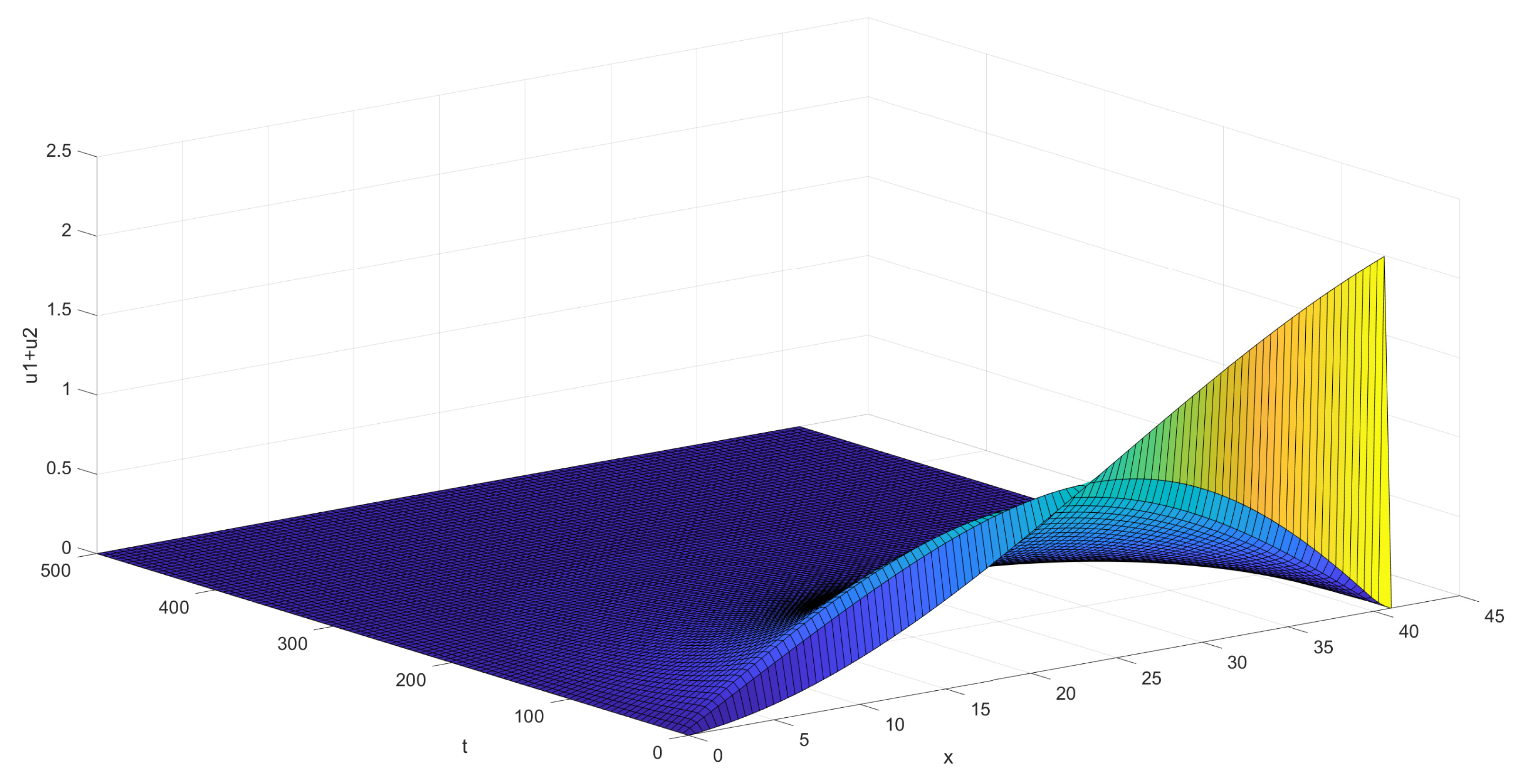
The first graph, Figure 4 below, shows the behavior of the sum of the coordinates of the solution $u_1+u_2$ for the situation given visually on Figure 3, in the case of just one pair of background and control zones. The initial function was taken as having both coordinates $sin(x/45)$.

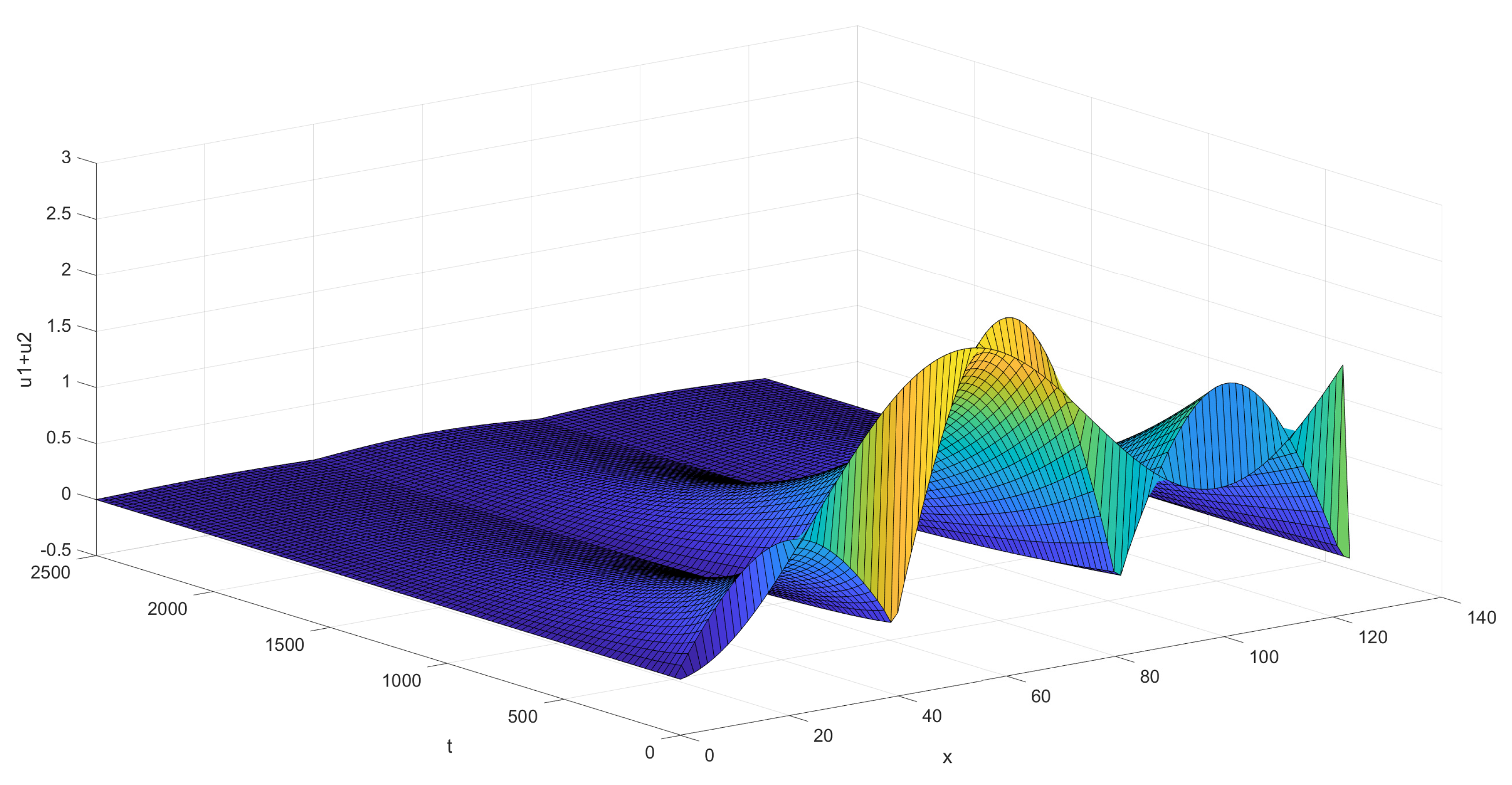
The second graph, Figure 5 below, shows the behavior of the sum of the coordinates of the solution $u_1+u_2$ for the situation given visually on Figure 3, in the case of three pairs of background and control zones. The process of dying out is seen to be slower on this much larger territory. Nevertheless the decay is seen to start rapidly after a short period of initial perturbations.

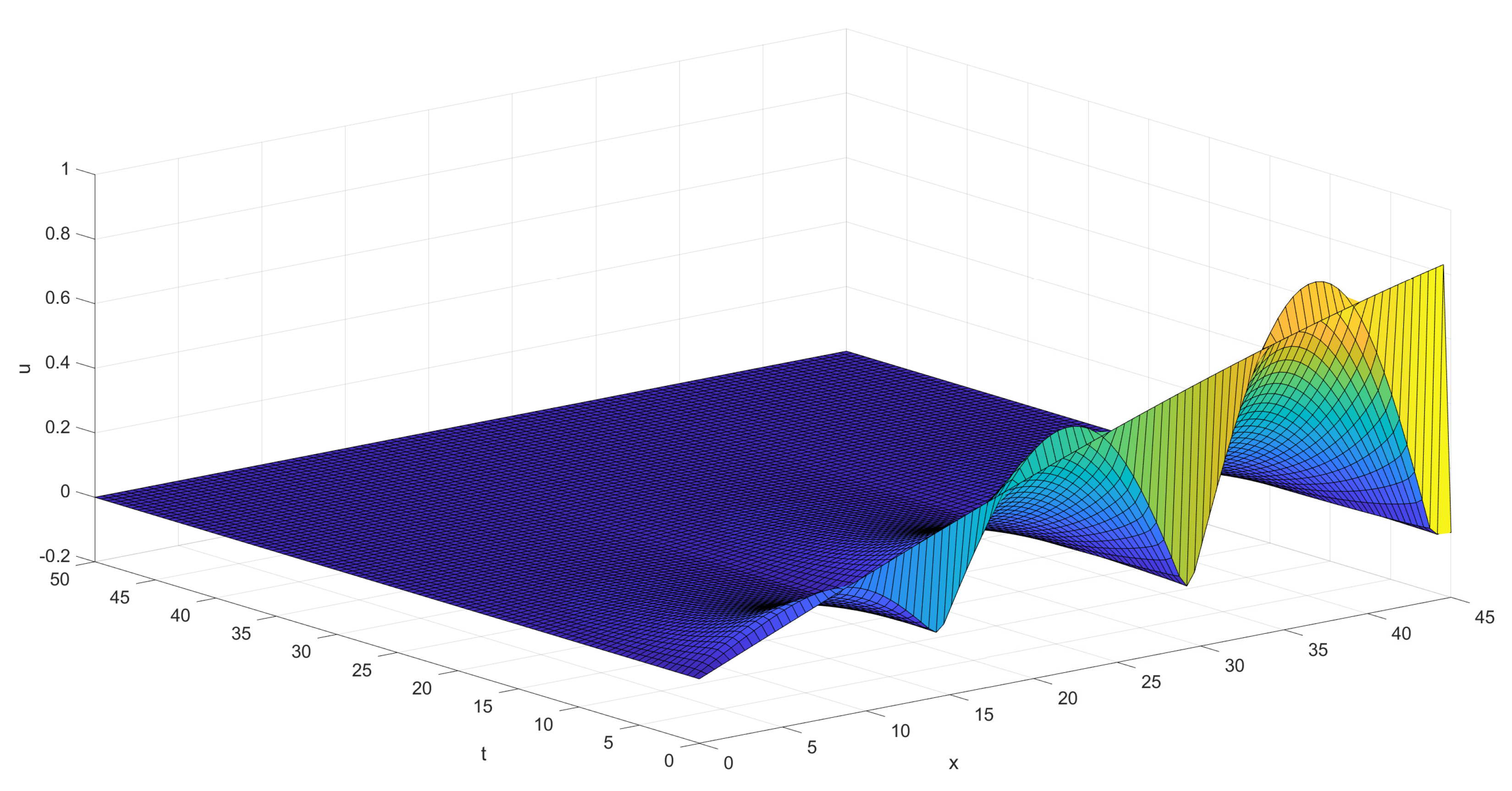
Finally we give a picture, Figure 6 below, illustrating the decay of ticks’ population in the simple model with all generations averaged out, which is visually presented on Figure 2. Again three pairs of background and control zones are used. The decay is seen to occur almost monotone and rather fast in this situation of rather poor complexity.

5. Proofs

Proof Theorem 1. 

Negativity of the operator L means that L has no non-negative eigenvalues. If such an eigenvalue E exists, then it solves the stationary problem $Ly=Ey$. Since the operator $y\to y^{″}$ with Dirichlet boundary conditions is negative, it follows that $E\in [0,\lambda )$. Then the general solutions in the two domains are

$$y_{ben}=Csin\left(\sqrt{\frac{\lambda -E}{a}}x\right)+Dcos\left(\sqrt{\frac{\lambda -E}{a}}x\right),x\in (0,R),$$

(39)

$$y_{nb}=Aexp\{\sqrt{\frac{\mu +E}{b}}x\}+Bexp\{-\sqrt{\frac{\mu +E}{b}}x\},x\in (R,R+r).$$

(40)

The Dirichlet boundary condition $y_{ben}\left(0\right)=0$ implies that $D=0$. Since eigenfunctions are defined up to a multiplicative constant, we can set $C=1$, so that

$$y_{ben}=sin\left(\sqrt{\frac{\lambda -E}{a}}x\right).$$

The Dirichlet boundary condition $y_{nb}(R+r)=0$ yields

$$B=-Aexp\{2\sqrt{\frac{\mu +E}{b}}(R+r)\}.$$

By the gluing conditions $y_{ben}\left(R\right)=y_{nb}\left(R\right)$ and $a{y}_{ben}^{\prime }\left(R\right)=b{y}_{nb}^{\prime }\left(R\right)$ on the interface,

$$sin\left(\sqrt{\frac{\lambda -E}{a}}R\right)=Aexp\{\sqrt{\frac{\mu +E}{b}}R\}+Bexp\{-\sqrt{\frac{\mu +E}{b}}R\},$$

$$\sqrt{a(\lambda -E)}cos\left(\sqrt{\frac{\lambda -E}{a}}x\right)=A\sqrt{b(\mu +E)}exp\{\sqrt{\frac{\mu +E}{b}}R\}-B\sqrt{b(\mu +E)}exp\{-\sqrt{\frac{\mu +E}{b}}R\}.$$

Thus

$$sin\left(\sqrt{\frac{\lambda -E}{a}}R\right)=A\left[exp\{\sqrt{\frac{\mu +E}{b}}R\}-exp\{\sqrt{\frac{\mu +E}{b}}(R+2r)\}\right],$$

$$\sqrt{a(\lambda -E)}cos\left(\sqrt{\frac{\lambda -E}{a}}x\right)$$

$$=A\sqrt{b(\mu +E)}\left[exp\{\sqrt{\frac{\mu +E}{b}}R\}+exp\{\sqrt{\frac{\mu +E}{b}}(R+2r)\}\right],$$

or

$$-\frac{tanh\left(r\sqrt{\frac{\mu +E}{b}}\right)}{\sqrt{b(\mu +E)}}=\frac{tan\left(\sqrt{\frac{\lambda -E}{a}}R\right)}{\sqrt{a(\lambda -E)}}.$$

Changing to $x=(\lambda -E)/a\in (0,\lambda /a]$ yields

$$-\frac{tanh\left(r\sqrt{(\lambda +\mu -ax)/b}\right)}{\sqrt{b(\lambda +\mu -ax)}}=\frac{tan\left(R\sqrt{x}\right)}{a\sqrt{x}}.$$

(41)

The l.h.s. is negative decreasing on $[0,\lambda /a]$. Thus, if $\lambda /a\le {\pi }^2/\left(4R^2\right)$, there are no solutions $x\in (0,\lambda /a]$, because the r.h.s. is positive on this interval.

Moreover, the l.h.s. is decreasing on $[0,\lambda /a]$ from

$$-\frac{tanh\left(r\sqrt{(\lambda +\mu )/b}\right)}{\sqrt{b(\lambda +\mu )}}\mathrm{to}-\frac{tanh\left(r\sqrt{\mu /b}\right)}{\sqrt{b\mu }}.$$

Thus, if $\lambda /a\ge {\pi }^2/R^2$, there is a solution $x\in (0,\lambda /a]$, because the l.h.s. necessarily intersects with the part of the r.h.s. increasing from $-\infty$ to 0. Finally, if

$$\frac{{\pi }^2}{4R^2}<\lambda /a<\frac{{\pi }^2}{R^2},$$

a solution exists if and only if the value of the l.h.s of (41) at $x=\lambda /a$ lies below the graph of the r.h.s. yielding condition (6). □

Proof of Theorem 2. 

Similar calculations to Theorem 1 show that the condition for $E\in [0,\lambda )$ to be an eigenvalue writes down as the equation

$$\sqrt{a(\lambda -E)}tan\left(\sqrt{\frac{\lambda -E}{a}}R\right)=\sqrt{b(\mu +E)}tanh\left(\sqrt{\frac{\mu +E}{b}}r\right),$$

(42)

or, in terms of $x=(\lambda -E)/a$, as

$$\sqrt{(\mu +\lambda -ax)b}tanh\left(r\sqrt{\frac{\mu +\lambda -ax}{b}}\right)=a\sqrt{x}tan\left(R\sqrt{x}\right).$$

(43)

The r.h.s. is positive increasing from 0 to ∞ on $[0,{\pi }^2/4R^2)$. The l.h.s. is positive decreasing on $[0,\lambda ]$ between two positive values (or between a positive value and 0 if $\mu =0$). Hence if

$$\lambda /a\ge {\pi }^2/{\left(2R\right)}^2,$$

there is a positive eigenvalue for any $\mu ,r$. Otherwise, a positive eigenvalue does not exist if and only (7) holds. □

Proof of Theorem 3. 

We again look at the system of equations

$${\dot{y}}_{ben}=a{y}_{ben}^{″}+\lambda y_{ben},{\dot{y}}_{nb}=b{y}_{nb}^{″}-\mu y_{nb}.$$

It is convenient to choose coordinates so that the first equation holds for $x\in (-R/2,R/2)$ and the second for $x\in (R/2,R/2+r)$. Here the key point for the analysis is the symmetry. Namely, our system writes down as the equation $\dot{y}=Ly$ on the torus $y\in [-(R+r)/2,(R+r)/2]$ with the identified right and left points. Alternatively one can think of y as periodic functions (with period $R+r$) on the whole $\mathbf{R}$. Here L is the linear operator such that $L\mathcal{R}=\mathcal{R}L$, where $\mathcal{R}$ is the reflection operator: $\mathcal{R}f\left(x\right)=f(-x)$. Hence if y is an eigenfunction of L, then so is also the function $\mathcal{R}y$. However, L is an operator of the Schrödinger type, and it is well known from quantum mechanics (and actually very easy to prove, see, e.g., [39]) that the eigenvalues of one-dimensional Scrödinger operators are non-degenerate, i.e., there may exist only one eigenfunction to each eigenvalue, up to a multiplier. Hence $\mathcal{R}y=\pm y$. However, the minus sign would contradict the continuity and thus $\mathcal{R}y=y$. Thus, an eigenfunction of L, which is the solution to the equation $LY=Ey$ must be an even function. Similarly it has to be symmetric under the reflection with respect to the point $(R+r)/2$.

The equation $Ly=Ey$ writes down more explicitly as the system

$$a{y}_{ben}^{″}+\lambda y_{ben}=E{y}_{ben},b{y}_{nb}^{″}-\mu y_{nb}=E{y}_{nb},$$

or equivalently

$$y_{ben}^{″}+\frac{\lambda -E}{a}{y}_{ben}=0,y_{nb}^{″}-\frac{\mu +E}{b}{y}_{nb}=0.$$

As usual we are looking for the solutions with $E\in [0,\lambda ]$. Then the functions $y_1$ and $y_2$ are of type (39) and (40) (now on intervals $(-R/2,R/2)$, $(-R/2,r+R/2)$).

However, it is easy to show that if

$$Asin\left(\sqrt{\lambda }(\xi +x)\right)+Bcos\left(\sqrt{\lambda }(\xi +x)\right)$$

is an even function of x, then it is of the form $Ccos\left(\sqrt{\lambda }x\right)$ (and the same holds for the linear combinations of sinh and cosh). Consequently, by the symmetry mentioned above, we can conclude that

$$y_{ben}=Acos\left(\sqrt{\frac{\lambda -E}{a}}x\right),y_{nb}=Bcosh\left(\sqrt{\frac{\mu +E}{b}}(x-(R+r)/2)\right).$$

Gluing the functions and their derivatives on the interface $x=R/2$ (recall (3)) yields

$$Acos\left(\sqrt{\frac{\lambda -E}{a}}\frac{R}{2}\right)=Bcosh\left(\sqrt{\frac{\mu +E}{b}}\frac{r}{2}\right),$$

$$Aa\sqrt{\frac{\lambda -E}{a}}sin\left(\sqrt{\frac{\lambda -E}{a}}\frac{R}{2}\right)=Bb\sqrt{\frac{\mu +E}{b}}sinh\left(\sqrt{\frac{\mu +E}{b}}\frac{r}{2}\right),$$

and thus

$$\sqrt{a(\lambda -E)}tan\left(\sqrt{\frac{\lambda -E}{a}}\frac{R}{2}\right)=\sqrt{b(\mu +E)}tanh\left(\sqrt{\frac{\mu +E}{b}}\frac{r}{2}\right),$$

which is the same as (42) but with $R/2$ and $r/2$ instead of R ad r. Hence the proof is completed as in Theorem 2. □

Proof of Theorem 4. 

Now a solution y to the eigenvalue problem $Ly=Ey$ is obtained by gluing solutions $y_{odd}$ and $y_{even}$ defined by formulas such as (39) and (40) on odd and even subintervals. The key point is, that under the periodic condition the operator L commutes with the shift operator $Tf\left(x\right)=f(x+R+r)$, where the addition is understood modulo $R+r$. This means that for any eigenfunction y of L, the function $Ty$ is also an eigenfunction with the same eigenvalue. Using the nondegeneracy of eigenvalues of L (as in the proof of the previous theorem) we can conclude that $Ty=\omega y$ for some $\omega$. However, $T^k$ is the identity operator, so that ${\omega }^k=1$. Since our eigenfunctions are real it follows that $\omega =\pm 1$. Again the multiplication by $-1$ would contradict the continuity and thus only $\omega =1$ is allowed. Hence we are directly in the setting of Theorem 3 and the proof is complete. □

Proof of Theorems 5 and 6. 

Under the conditions of the Theorems, there exists an invertible matrix C such that $CM{C}^{-1}=D$ is diagonal with the elements ${\mathrm{\Lambda }}_j$ on the diagonal. Then in the variables $z=Cy$ all equations and boundary conditions remain the same, but with M substituted by D. Hence our system decomposes into n independent equations for the coordinates $z^j$ of the vector-valued function z. For all $z^j$ with $j>1$ there can be no positive eigenvalues, because all operators involved are strictly negative. Furthermore, the equations for $z^1$ (and all boundary conditions) become identical to the equations for y of the one-dimensional case, with ${\mathrm{\Lambda }}_1$ instead of $\lambda$ and the new $\mu$ being equal to $\lambda +\mu$ of the one-dimensional case. □

Proof of Theorem 7. 

The eigenvalue problem to Equation (18) with the Dirichlet boundary condition writes down as $A{y}^{″}+My=Ey$ subject to $y\left(0\right)=y\left(R\right)=0$. Equivalently this equation rewrites as

$$y^{″}+(A^{-1}M-A^{-1}E)y=0.$$

(44)

It is easy to see that the highest real eigenvalue of the matrix $A^{-1}M-A^{-1}E$ decreases with the increase of E. Hence, according to Theorem 5, Equation (44) is solvable for some positive E if and only if the highest real eigenvalue ${\mathrm{\Lambda }}_1$ of the matrix $A^{-1}M$ satisfies the condition ${\mathrm{\Lambda }}_1>{\pi }^2/R^2$ implying the claim of the theorem. □

Proof of Theorem 8. 

Change the variable in (20) to z so that to $z_{ben}=A_{ben}y$, $z_{nb}=A_{nb}y$. Then we obtain

$$\begin{array}{cc}\hfill & z_{ben}^{″}+(M_{ben}-E)A_{ben}^{-1}{z}_{ben}=0\hfill \\ \hfill & z_{nb}^{″}+(M_{nb}-E)A_{nb}^{-1}{z}_{nb}=0,\hfill \end{array}$$

(45)

and the gluing condition for z is the continuity of z and $z^{\prime }$ on the interfaces.

Let $L\left(E\right)$ denote the operator on the r.h.s. of (45), so that system (45) can be concisely written as $L\left(E\right)z=0$. We are interested in a criterion that ensures that this equation has no solution with $E\ge 0$. This would be the case, if one could show that $(z,L(E\left)z\right)<0$ for all z. However, $(z,L\left(E\right)z)=(z,L^S\left(E\right)z)$, where $L^S\left(E\right)=(L\left(E\right)+L^T\left(E\right))/2$ is the symmetrization. Thus, it is sufficient to show that $L^S\left(E\right)$ is a negative symmetric operator for any positive E. However, $L^S\left(E\right)$ decreases with the increase of E. Thus it is sufficient to show that $L=L\left(0\right)$ is negative, i.e., $Lz=Pz$ has no solutions with non-negative P.

Furthermore, this means that there are no solutions to the system

$$\begin{array}{cc}\hfill & z_{ben}^{″}+(M_{ben}^S-P)z_{ben}=0\hfill \\ \hfill & z_{nb}^{″}+(M_{nb}^S-P)z_{nb}=0,\hfill \end{array}$$

(46)

with $P\ge 0$ and $M_{ben}^S=(M_{ben}{A}_{ben}^{-1}+A_{ben}^{-1}{M}_{ben}^T)/2$, $M_{nb}^S=(M_{nb}{A}_{nb}^{-1}+A_{nb}^{-1}{M}_{nb}^T)/2$.

It is clear that the required sufficient condition is sufficient to show for the case when all eigenvalues of $M_{ben}^S$ and $M_{nb}^S$ are different, as the general case is obtained by a straightforward limiting procedure.

For simplicity, let us assume that $M_{ben}^S$ has one positive eigenvalue (i.e., $k=1$) and all other are negative: ${\lambda }_1>0\ge {\lambda }_2>\cdots >{\lambda }_n$.

Clearly $P\ge {\lambda }_1$ are impossible in (46), so that only $P\in [0,{\lambda }_1]$ have to be analyzed.

Due to the periodic conditions, solutions to (46) are given by the formulas (see beginning of the proof of Theorem 3)

$$z_{ben}=A_{1}cos\left(\sqrt{{\lambda }_1-P}x\right)v_1+\sum _{j=2}^n{A}_{j}cosh\left(\sqrt{P-{\lambda }_j}x\right)v_j,$$

$$z_{nb}=\sum _{j=1}^n{B}_{j}cosh\left(\sqrt{P-{\mu }_j}(x-(R+r)/2)\right)w_j,$$

where $v_j$ and $w_j$ are orthonormal spectral bases for $M_{ben}^S$ and $M_{nb}^S$.

Let $w_j={\sum }_k{c}_{jk}{v}_k$ with an orthogonal matrix $C=\left(c_{ij}\right)$. Then

$$z_{nb}=\sum B_{k}cosh\left(\sqrt{P-{\mu }_k}(x-(R+r)/2)\right)c_{kj}{v}_j.$$

Thus, gluing $z_{ben}$ and $z_{nb}$ at $x=R/2$ yields

$$A_{1}cos(\sqrt{{\lambda }_1-P}R/2)=\sum _j{B}_{j}cosh(\sqrt{P-{\mu }_j}r/2)c_{j1},$$

and

$$A_{i}cosh(\sqrt{P-{\lambda }_j}R/2)=\sum _j{B}_{j}cosh(\sqrt{P-{\mu }_j}r/2)c_{ji},i>1.$$

Next, since

$${\int }_{-R/2}^{r+R/2}(z\left(x\right),z^{″}\left(x\right))dx=-{\int }_{-R/2}^{r+R/2}(z^{\prime }\left(x\right),z^{\prime }\left(x\right))dx,$$

which follows from the integration by parts and the gluing (and periodic) conditions, we have that, for a solution to (46),

$$0\le {\int }_{ben}(z_{ben},(M_{ben}^S-P)z_{ben})dx+{\int }_{nb}(z_{nb},(M_{nb}^S-P)z_{nb})dx$$

$$=A_1^2({\lambda }_1-P){\int }_{ben}{cos}^2\left(\sqrt{{\lambda }_1-P}x\right)dx+\sum _{j>1}{A}_j^2({\lambda }_j-P){\int }_{ben}{cosh}^2\left(\sqrt{P-{\lambda }_j}x\right)dx$$

$$+\sum _{j\ge 1}{B}_j^2({\mu }_j-P){\int }_{nb}{cosh}^2\left(\sqrt{P-{\mu }_j}(x-(R+r)/2)\right)dx.$$

Since $cos\left(2x\right)=2{cos}^{2}x-1$ and $cosh\left(2x\right)=2{cosh}^{2}x-1$,

$${\int }_{\xi }^{\xi }{cos}^2\left(\alpha x\right)dx=\xi +\frac{1}{2}{\int }_{\xi }^{\xi }cos\left(2\alpha x\right)dx=\xi +\frac{sin\left(2\alpha \xi \right)}{2\alpha },$$

and thus

$$A_1^2({\lambda }_1-P)\left(\frac{R}{2}+\frac{sin\left(R\sqrt{{\lambda }_1-P}\right)}{2\sqrt{{\lambda }_1-P}}\right)\ge \sum _{j\ge 1}{B}_j^2(P-{\mu }_j)\left(\frac{r}{2}+\frac{sinh\left(r\sqrt{P-{\mu }_j}\right)}{2\sqrt{P-{\mu }_j}}\right).$$

(47)

In particular,

$$A_1^2\ge B_j^2\frac{P-{\mu }_j}{{\lambda }_1-P}\frac{\left(\frac{r}{2}+\frac{sinh\left(r\sqrt{P-{\mu }_j}\right)}{2\sqrt{P-{\mu }_j}}\right)}{\left(\frac{R}{2}+\frac{sin\left(R\sqrt{{\lambda }_1-P}\right)}{2\sqrt{{\lambda }_1-P}}\right)}$$

for any j.

One could work with this estimate, but it makes the final result more transparent (though a bit rougher), if one simplifies this estimate to the following one:

$$A_1^2\ge B_j^2\frac{\sqrt{P-{\mu }_j}sinh\left(r\sqrt{P-{\mu }_j}\right)}{2R({\lambda }_1-P)}.$$

On the other hand,

$$|A_1|cos\left(\sqrt{{\lambda }_1-P}\frac{R}{2}\right)\le \sum _j\left|B_j\right|cosh\left(\sqrt{P-{\mu }_j}\frac{r}{2}\right)c_{j1},$$

and thus

$$A_1^2{cos}^2\left(\sqrt{{\lambda }_1-P}\frac{R}{2}\right)\le n\sum _j{B}_j^2{cosh}^2\left(\sqrt{P-{\mu }_j}\frac{r}{2}\right)c_{j1}^2\le n\underset{j}{max}{B}_j^2{cosh}^2\left(\sqrt{P-{\mu }_j}\frac{r}{2}\right),$$

or

$$A_1^2(1+cos\left(\sqrt{{\lambda }_1-P}R\right))\le n\underset{j}{max}{B}_j^2(1+cosh\left(\sqrt{P-{\mu }_j}r\right)).$$

Thus, for a j realizing the maximum we have

$$n\frac{1+cosh\left(\sqrt{P-{\mu }_j}r\right)}{1+cos\left(\sqrt{{\lambda }_1-P}R\right)}\ge \frac{\sqrt{P-{\mu }_j}sinh\left(r\sqrt{P-{\mu }_j}\right)}{2R({\lambda }_1-P)},$$

or

$$\frac{R({\lambda }_1-P)}{(1+cos\left(R\sqrt{{\lambda }_1-P}\right))}\ge \frac{\sqrt{P-{\mu }_j}sinh\left(r\sqrt{P-{\mu }_j}\right)}{2n(1+cosh\left(r\sqrt{P-{\mu }_j}\right))}.$$

(48)

This can be rewritten as

$$\frac{1}{R}{g}_1\left(R\sqrt{{\lambda }_1-P}\right)\ge \frac{1}{2nr}{g}_2\left(r\sqrt{P-{\mu }_j}\right)$$

(49)

with

$$g_1\left(x\right)=\frac{x^2}{1+cosx},g_2\left(x\right)=\frac{xsinhx}{1+coshx}.$$

(50)

In order to make (49) impossible (and thus to ensure the negativity of our operator) it is sufficient to assume that

$$\frac{1}{R}{g}_1\left(R\sqrt{x}\right)<\frac{1}{2nr}{g}_2\left(r\sqrt{{\lambda }_1-{\mu }_1-x}\right)$$

(51)

for $x\in [0,{\lambda }_1]$, where $x={\lambda }_1-P$. For ${\lambda }_1\ge {\pi }^2/R$, this cannot be true. Hence assume ${\lambda }_1<{\pi }^2/R$.

Since it is straightforward to check that the function

$$\frac{g_1\left(R\sqrt{x}\right)}{g_2\left(r\sqrt{{\lambda }_1-{\mu }_1-x}\right)}$$

is increasing for $x\in [0,{\lambda }_1]$, condition (51) is equivalent to this condition on the endpoint:

$$\frac{1}{R}{g}_1\left(R\sqrt{{\lambda }_1}\right)<\frac{1}{2nr}{g}_2\left(r\sqrt{|{\mu }_1|}\right),$$

(52)

or explicitly

$$\frac{2Rn{\lambda }_1}{1+cos\left(R\sqrt{{\lambda }_1}\right))}<\frac{\sqrt{|{\mu }_1|}sinh\left(r\sqrt{|{\mu }_1|}\right)}{1+cosh\left(r\sqrt{|{\mu }_1|}\right)},$$

(53)

which coincides with (22) for $k=1$.

Modifications required for arbitrary k are straightforward, and we omit them. □

Proof of Theorem 9. 

The eigenvalue Equation (25) can be written as

$$\begin{array}{cc}\hfill & y_{ben}^{″}+N_{ben}\left(E\right)y_{ben}=0\hfill \\ \hfill & y_{nb}^{″}+N_{nb}\left(E\right)y_{nb}=0.\hfill \end{array}$$

(54)

As above we can write

$$y_{ben}=Acos\left(\sqrt{{\mathrm{\Lambda }}_1}x\right)v_1+Bcosh\left(\sqrt{|{\mathrm{\Lambda }}_2|}x\right)v_2,$$

$$y_{nb}=Ccosh\left(\sqrt{|{\mu }_1|}(x-(R+r)/2)\right)w_1+Dcosh\left(\sqrt{|{\mu }_2|}(x-(R+r)/2)\right)w_2.$$

The last equation is rewritten as

$$y_{nb}=Ccosh\left(\sqrt{|{\mu }_1|}(x-(R+r)/2)\right)(c_{11}{v}_1+c_{12}{v}_2)+Dcosh\left(\sqrt{|{\mu }_2|}(x-(R+r)/2)\right)(c_{21}{v}_1+c_{22}{v}_2).$$

Evidently, all terms here depend on E.

Furthermore, in order to shorten the formulas, we shall write sin, cos, tan if the argument is $\sqrt{{\mathrm{\Lambda }}_1}R/2$ and sinh, cosh, tanh if the argument is $\sqrt{|{\mathrm{\Lambda }}_2|}R/2$. Gluing the solutions at the interface $x=R$ yields

$$Acos=Ccosh(\sqrt{|{\mu }_1|}r/2)c_{11}+Dcosh(\sqrt{|{\mu }_2|}r/2)c_{21},$$

$$Bcosh=Ccosh(\sqrt{|{\mu }_1|}r/2)c_{12}+Dcosh(\sqrt{|{\mu }_2|}r/2)c_{22}.$$

and

$$-A\sqrt{{\mathrm{\Lambda }}_1}sin=-a(C\sqrt{|{\mu }_1|}sinh(\sqrt{|{\mu }_1|}r/2)c_{11}+D\sqrt{|{\mu }_2|}sinh(\sqrt{|{\mu }_2|}r/2)c_{21}),$$

$$B\sqrt{{\mathrm{\Lambda }}_1}sinh=-a(C\sqrt{|{\mu }_1|}sinh(\sqrt{|{\mu }_1|}r/2)c_{12}+D\sqrt{|{\mu }_2|}sinh(\sqrt{|{\mu }_2|}r/2)c_{22}).$$

Equalising A from the 1st equations yields

$$\sqrt{{\mathrm{\Lambda }}_1}tan[Ccosh(\sqrt{|{\mu }_1|}r/2)c_{11}+Dcosh(\sqrt{|{\mu }_2|}r/2)c_{21}]$$

$$=a[C\sqrt{|{\mu }_1|}sinh(\sqrt{|{\mu }_1|}r/2)c_{11}+D\sqrt{|{\mu }_2|}sinh(\sqrt{|{\mu }_2|}r/2)c_{21}].$$

Equalising B from the 2nd equations yields

$$\sqrt{|{\mathrm{\Lambda }}_2|}tanh[Ccosh(\sqrt{|{\mu }_1|}r/2)c_{12}+Dcosh(\sqrt{|{\mu }_2|}r/2)c_{22}]$$

$$=-a[C\sqrt{|{\mu }_1|}sinh(\sqrt{|{\mu }_1|}r/2)c_{12}+D\sqrt{|{\mu }_2|}sinh(\sqrt{|{\mu }_2|}r/2)c_{22}].$$

The condition for the existence of a solution to this system of two equations with two unknown $C,D$ writes down as the equation

$$c_{11}{c}_{22}[\sqrt{{\mathrm{\Lambda }}_1}tan-a\sqrt{|{\mu }_1|}tanh(\sqrt{|{\mu }_1|}r/2)][\sqrt{|{\mathrm{\Lambda }}_2|}tanh+a\sqrt{|{\mu }_2|}tanh(\sqrt{|{\mu }_2|}r/2)]$$

$$-c_{12}{c}_{21}[\sqrt{{\mathrm{\Lambda }}_1}tan-a\sqrt{|{\mu }_2|}tanh(\sqrt{|{\mu }_2|}r/2)][\sqrt{|{\mathrm{\Lambda }}_2|}tanh+a\sqrt{|{\mu }_1|}tanh(\sqrt{|{\mu }_1|}r/2)]=0,$$

or as ${\sqrt{\mathrm{\Lambda }}}_{1}tan=aB/A$ with

$$A=c_{11}{c}_{22}[\sqrt{|{\mathrm{\Lambda }}_2|}tanh+a\sqrt{|{\mu }_2|}tanh(\sqrt{|{\mu }_2|}r/2)]$$

$$-c_{12}{c}_{21}[\sqrt{|{\mathrm{\Lambda }}_2|}tanh+a\sqrt{|{\mu }_1|}tanh(\sqrt{|{\mu }_1|}r/2)],$$

$$B=c_{11}{c}_{22}\sqrt{|{\mu }_1|}tanh(\sqrt{|{\mu }_1|}r/2)[\sqrt{|{\mathrm{\Lambda }}_2|}tanh+a\sqrt{|{\mu }_2|}tanh(\sqrt{|{\mu }_2|}r/2)]$$

$$-c_{12}{c}_{21}\sqrt{|{\mu }_2|}tanh(\sqrt{|{\mu }_2|}r/2)][\sqrt{|{\mathrm{\Lambda }}_2|}tanh+a\sqrt{|{\mu }_1|}tanh(\sqrt{|{\mu }_1|}r/2)].$$

Since $c_{12}{c}_{21}\le 0$ and $c_{11}{c}_{22}\ge 0$ (and $|{\mu }_2|\ge |{\mu }_1\left|\right)$, it follows that

$$B\ge detc[a\sqrt{|{\mu }_2|}tanh(\sqrt{|{\mu }_2|}r/2)+\sqrt{{\mathrm{\Lambda }}_2}tanh]\sqrt{|{\mu }_1|}tanh(\sqrt{|{\mu }_1|}r/2),$$

$$0<A<detc[\sqrt{|{\mathrm{\Lambda }}_2|}tanh+a\sqrt{|{\mu }_2|}tanh(\sqrt{|{\mu }_2|}r/2)],$$

so that

$$aB/A\ge a\sqrt{|{\mu }_1|}tanh(\sqrt{|{\mu }_1|}r/2).$$

(55)

Hence

$$\sqrt{{\mathrm{\Lambda }}_1}tan(\sqrt{{\lambda }_1}R/2)\ge a\sqrt{|{\mu }_1|}tanh(\sqrt{|{\mu }_1|}r/2).$$

Consequently, if (27) holds, this is impossible. It remains to notice that, by monotonicity, this condition holds for all E if and only if it holds for $E=0$. □

Proof of Theorem 10. 

As is easily seen, if inequalities (30) hold for $N_{ben}\left(0\right)$ and $N_{nb}\left(0\right)$, then they hold for $N_{ben}\left(E\right)$ and $N_{nb}\left(E\right)$ with all positive E. Hence it is sufficient to check condition (26) for $E=0$.

For a matrix

$$A=\left(\begin{array}{c}-m_1{b}_1\hfill \\ b_2-m_2\hfill \end{array}\right),$$

the eigenvalues are

$${\mathrm{\Lambda }}_{1,2}=\frac{1}{2}\left[-(m_1+m_2)\pm \sqrt{{(m_1-m_2)}^2+4b_1{b}_2}\right].$$

Thus, ${\mathrm{\Lambda }}_2<0$ and ${\mathrm{\Lambda }}_1>0$.

Looking for eigenvectors $v_{1,2}$, let us choose $v_1^1=1,v_2^2=1$. Then

$$v_1^2=\frac{{\mathrm{\Lambda }}_1+m_1}{b_1}=\frac{b_2}{{\mathrm{\Lambda }}_1+m_2},$$

$$v_2^1=\frac{b_1}{{\mathrm{\Lambda }}_2+m_1}=\frac{{\mathrm{\Lambda }}_2+m_2}{b_2}.$$

Thus

$$V=\left(\begin{array}{c}1v_2^1\hfill \\ v_1^{2}1\hfill \end{array}\right),W=\left(\begin{array}{c}1w_2^1\hfill \\ w_1^{2}1\hfill \end{array}\right).$$

Consequently,

$$C=W{V}^{-1}=\frac{1}{detV}\left(\begin{array}{c}1-v_2^1{w}_1^2{w}_2^1-v_2^1\hfill \\ -v_1^2+w_1^{2}1-v_1^2{w}_2^1\hfill \end{array}\right).$$

Assuming $m_1>m_2$, we see that

$$v_2^1=-\frac{(m_1-m_2)+\sqrt{{(m_1-m_2)}^2+4b_1{b}_2}}{2b_2}<0,$$

$$v_1^2=\frac{(m_1-m_2)+\sqrt{{(m_1-m_2)}^2+4b_1{b}_2}}{2b_1}<0.$$

Similarly, $w_2^1<0$ and $w_1^2>0$. They have the same expression, but with ${\tilde{m}}_j$ and ${\tilde{b}}_j$ instead of $m_j,b_j$. Hence $c_{11},c_{22}\ge 1>0$. Moreover,

$$c_{12}{c}_{21}=-(w_1^2-v_1^2)\left(\right|w_2^1|-|v_2^1\left|\right).$$

Under (28) and (29), it follows that, for any $\omega \in (0,1)$,

$$w_1^2\ge v_1^2,|w_2^1|\ge |v_2^1|,$$

and thus $c_{12}{c}_{21}<0$, which completes the proof. □

6. Conclusions

In this paper, we developed the diffusion model for the propagation of ticks with variable discontinuous diffusion coefficients. We extended the famous KISS model (originated in plankton research) to describe the dynamics on patchy territories with intermittent background (beneficial) and control (non-beneficial) zones and gave conditions for the control parameters that ensure the eradication of ticks’ population. Mathematically, these conditions imply the negativity of the corresponding diffusion operator. We started with rather trivial (though complete) results for the scalar case (one-stage populations) and then presented some advanced theorems for the vector-valued non-symmetric diffusions stressing serious theoretical difficulties that arise in this extension. Finally we used various published resources reporting on the concrete observations of ticks in order to extract some concrete numeric values for the parameters of background zones and thus to provide approximate numeric values to the required parameters of the control zones. In particular, we found that the roughest scalar model yields closer values of about 16 km for the KISS critical patch sizes related to both the lone star and the taiga ticks. On the other hand, using more detailed information combined with a more detailed multi-stage model can provide quite different output parameters. Furthermore, concrete numeric data showed that the estimates based on the symmetrization of the birth-and-death matrix (vary natural from the theoretical point of view) can underestimate strongly the lower bounds for the KISS scales.

Let us note some further perspectives. We used in this paper a one-dimensional diffusion model aiming at the approximate description of the propagation in a certain direction. Evidently, it would be natural to extend the results to a more realistic (for ticks and many other species) two-dimensional diffusion model. On the other hand, we discussed the solutions in a global closed territory. Of interest would be a more local analysis of the solutions in a (possibly intermittent) small territory placed in contact with a large reservoir of an expanding background population. Such solutions could be possibly analyzed based on the Fokas method, see [38,40], or via the method of estimating the heat content, see, e.g., [41]. It would be also of interest to see whether the results of Theorem 9 have any reasonable extensions beyond the restrictive assumptions (26) and whether one can obtain some multi-dimensional analogs. Furthermore, Remark 5 can be used for practical calculations with multi-dimensional models. A realistic vector-valued diffusion model can include not only ticks in various stages, but also the hosts.

Practically, the main goal of this paper was to give exact recommendations on the properties of control zones needed for the eradication of ticks. However, the numbers obtained in our analysis are based on very rough estimates, and our calculations show that they are quite sensitive to the input data. A much more detailed program of concrete observations in various places is needed to make the estimates more precise and more specific for concrete regions.

In this paper, we only used the diffusion models. Further investigations are needed to see whether more appropriate approximations can be achieved using other models, such as the telegraph equations, or presently very popular sub-diffusions or super-diffusions.

Please note finally that our models with periodic intermittent beneficial/non-beneficial zones present much simplified versions of the parabolic Anderson models with random potentials, to which an immense number of studies were devoted, see, e.g., [42] and references therein.

References

- Gaff, H.D.; Gross, L.J. Modeling Tick-Borne Disease: A Metapopulation Model. Bull. Math. Biol. 2007, 69, 265–288. [Google Scholar] [CrossRef]
- White, A.; Schaefer, E.; Thompson, C.W.; Kribs, C.M.; Gaff, H. Dynamics of two pathogens in a single tick population. Lett. Biomath. 2019, 6, 50–66. [Google Scholar] [CrossRef]
- Nah, K.; Wu, J. Long-term transmission dynamics of tick-borne diseases involving seasonal variation and co-feeding transmission. J. Biol. Dyn. 2021, 15, 269–286. [Google Scholar] [CrossRef]
- Switkes, J.; Nannyonga, B.; Mugisha, J.Y.T.; Nakakawa, J. A mathematical model for Crimean-Congo haemorrhagic fever: Tick-borne dynamics with conferred host immunity. J. Biol. Dyn. 2016, 10, 59–70. [Google Scholar] [CrossRef] [Green Version]
- Zhang, X.; Sun, B.; Lou, Y. Dynamics of a periodic tick-borne disease model with co-feeding and multiple patches. J. Math. Biol. 2021, 82, 27. [Google Scholar] [CrossRef]
- dos Santos, J.P.C.; Cardoso, L.C.; Monteiro, E.; Lemes, N.H.T. A Fractional-Order Epidemic Model for Bovine Babesiosis Disease and Tick Populations. In Abstract and Applied Analysis; Hindawi: London, UK, 2015. [Google Scholar]
- Maliyoni, M.; Chirove, F.; Gaff, H.D.; Govinder, K.S. A Stochastic Tick-Borne Disease Model: Exploring the Probability of Pathogen Persistence. Bull. Math. Biol. 2017, 79, 1999–2021. [Google Scholar] [CrossRef]
- Gaff, H.D.; Schaefer, E.; Lenhart, S. Use of optimal control models to predict treatment time for managing tick-borne disease. J. Biol. Dyn. 2011, 5, 517–530. [Google Scholar] [CrossRef] [Green Version]
- Kashkynbayev, A.; Koptleuova, D. Global dynamics of tick-borne diseases. Math. Biosci. Eng. (MBE) 2020, 17, 4064–4079. [Google Scholar] [CrossRef]
- Shu, H.; Xu, W.; Wang, X.-S.; Wu, J. Complex dynamics in a delay differential equation with two delays in tick growth with diapause. J. Differ. Equ. 2020, 269, 10937–10963. [Google Scholar] [CrossRef]
- Vshivkova, O.A.; Komarov, A.S.; Frolov, P.V.; Khlebopros, R.G. The role of the heterogeneity of the habitat under the control of the ixode ticks number: Cellular-automaton model. Control Sci. 2013, 4, 57–63. (In Russian) [Google Scholar]
- Mwambi, H.G.; Baumgärtner, J.; Hadeler, K.P. Development of a stage-structured analytical population model for strategic decision making: The case of ticks and tick-borne diseases. Riv. Mat. Univ. Parma 2000, 3, 157–169. [Google Scholar]
- Tosato, M.; Nah, K.; Wu, J. Are host control strategies effective to eradicate tick-borne diseases (TBD)? J. Theor. Biol. 2021, 508, 110483. [Google Scholar] [CrossRef]
- Caraco, T.; Glavanakov, S.; Chen, G.; Flaherty, J.; Ohsumi, T.K.; Szymanski, B.K. Stage-structured infection transmission and a spatial epidemic: A model for Lyme disease. Am. Nat. 2002, 160, 348–359. [Google Scholar] [CrossRef]
- Caraco, T.; Gardener, G.; Maniatty, W.; Deelman, E.; Szymanski, B.K. Lyme Disease: Self regulation and Pathogen Invasion. J. Theor. Biol. 1998, 193, 561–575. [Google Scholar] [CrossRef]
- Zhao, X. Global dynamics of a reaction and diffusion model for Lyme disease. J. Math. Biol. 2012, 65, 787–808. [Google Scholar] [CrossRef]
- Holmes, E.E. Are diffusion models too simple? A comparison with telegraph models of invasion. Am. Nat. 1993, 142, 779–795. [Google Scholar] [CrossRef]
- Holmes, E.E.; Lewis, M.A.; Banks, J.E.; Veit, R.R. Partial differential equations in ecology: Spatial interactions and population dynamics. Ecology 1994, 75, 17–29. [Google Scholar] [CrossRef]
- Frassu, S.; Galván, R.R.; Viglialoro, G. Uniform in time L∞-estimates for an attraction-repulsion chemotaxis model with double saturation. Discret. Contin. Dyn. Syst. Ser. B 2022, 28, 1886–1904. [Google Scholar] [CrossRef]
- Frassu, S.; Li, T.; Viglialoro, G. Improvements and generalizations of results concerning attraction-repulsion chemotaxis models. Math. Methods Appl. Sci. 2022, 45, 11067–11078. [Google Scholar] [CrossRef]
- Kierstead, H.; Slobodkin, L.B. The Size of Water Masses Containing Plankton Bloom. J. Mar. Res. 1953, 12, 141–147. [Google Scholar]
- Skellam, J.G. Random Dispersal in theoretical biology. Bull. Math. Biol. 1991, 53, 135–165, Reprinted from Biometrika 1951, 38, 196–218. [Google Scholar] [CrossRef]
- Okubo, A. Critical patch size for plankton and patchiness. In Mathematical Ecology; Levin, S.A., Hallam, T.G., Eds.; Lecture Notes in Biomathematics 54; Springer: Berlin/Heidelberg, Germany, 1986; pp. 456–477. [Google Scholar]
- Murray, J.D. Mathematical Biology II: Spatial Models and Biomedical Applications, 3rd ed.; Springer: Berlin/Heidelberg, Germany, 2003. [Google Scholar]
- Baron, J.W.; Galla, T. Dispersal-induced instability in complex ecosystems. Nat. Commun. 2020, 11, 6032. [Google Scholar] [CrossRef]
- Gourley, S.A.; Britton, N.F.; Chaplain, M.A.J.; Byrne, H.M. Mechanisms for stabilisation and destabilisation of systems of reaction-diffusion equations. J. Math. Biol. 1996, 34, 857–877. [Google Scholar] [CrossRef]
- Mimura, M.; Murray, J.D. On a Diffusive Prey-Predator Model which Exhibits Patchiness. J. Theor. Biol. 1978, 75, 249–262. [Google Scholar] [CrossRef] [PubMed]
- Filippova, N.A. (Ed.) Taiga Tick Ixodes Persulcatus Schulze (Acarina, Ixodidae): Morphology, Systematics, Ecology, Medical Significance; Nauka: Moscow, Russia, 1985. (In Russian) [Google Scholar]
- Gaff, H.D.; White, A.; Leas, K.; Kelman, P.; Squire, J.C.; Livingston, D.L.; Sullivan, G.A.; Baker, E.W.; Sonenshine, D.E. TickBot: A novel robotic device for controlling tick populations in the natural environment. Ticks Tick-Borne Dis. 2015, 6, 146–151. [Google Scholar] [CrossRef] [PubMed]
- Mount, G.A.; Halle, D.G.; Barnard, D.R.; Daniels, E. New Version of LSTSIM for Computer Simulation of Amblyomma americanum (Acari: Ixodidae) Population Dynamics. J. Med. Entomol. 1993, 30, 843–857. [Google Scholar] [CrossRef] [PubMed]
- Ostfeld, R.S. The Ecology of Lyme-Disease Risk: Complex interactions between seemingly unconnected phenomena determine risks of exposure to this expanding disease. Am. Sci. 1997, 85, 338–346. [Google Scholar]
- Harris, G.W.; Burns, E.C. Predation on the lone star tick by the imported fire ant. Environ. Entomol. 1972, 1, 362–365. [Google Scholar] [CrossRef]
- Vshivkova, O.A. Mathematical simulation of ant influence on the ixode ticks number in Euroasian ecosystems. Izvestia Samarskogo Nauchnogo Cent. Russ. Acad. Sci. 2009, 11, 1631–1633. (In Russian) [Google Scholar]
- Fefferman, C.L. The uncertainty principle. Bulletin of the Americal Math. Society 1983, 9, 129–206. [Google Scholar]
- Sweezy, C. Relating different conditions for the positivity of the Schrödinger operator. Rocky Mt. J. Maths. 1993, 23, 353–366. [Google Scholar] [CrossRef]
- Mount, G.A.; Halle, D.G.; Daniels, E. Simulation of Blacklegged Tick (Acari: Ixodidae) Population Dynamics and Transmission of Borrelia burgdorferi. J. Med. Entomol. 1997, 34, 461–484. [Google Scholar] [CrossRef] [PubMed]
- Korotkov, U.S. Life cycle of the taiga tick Ixodes Persulcatus in the conifer forests of the bottom land of the East Sayan mountain range. Parasotologya 2014, 48, 20–36. (In Russuan) [Google Scholar]
- Sheils, N.E.; Deconinck, B. Initial-to-Interface Maps for the Heat Equation on Composite Domains. Stud. Appl. Math. 2016, 137, 140–154. [Google Scholar] [CrossRef] [Green Version]
- Landau, L.D.; Lifshitz, E.M. Quantum Mechanics, 2nd ed.; Pergamon Press: Oxford, UK, 1965. [Google Scholar]
- Fokas, A.S. A Unified Approach to Boundary Value Problems; SIAM: Philadelphia, PA, USA, 2008. [Google Scholar]
- Berg, M.v.; Gittins, K. Uniform bounds for the heat content of open sets in Euclidean space. Differ. Geom. Appl. 2015, 40, 67–85. [Google Scholar] [CrossRef]
- Makarova, Y.; Han, D.; Molchanov, S.; Yarovaya, E. Branching random walks with immigration. Lyapunov stability. Markov Process. Relat. Fields 2019, 25, 683–708. [Google Scholar]
Figure 1.
General scheme of periodic control zones.
Figure 2.
Parameters of control zones for lone star ticks under a simple model.
Figure 3.
Parameters of control zones for taiga ticks under a two-stage model.
Figure 4.
Decay of ticks in the case of one pair of background/control zones.
Figure 5.
Decay of ticks in the case of three pairs of background/control zones.
Figure 6.
Decay in the simplest one-stage model.
Disclaimer/Publisher’s Note: The statements, opinions and data contained in all publications are solely those of the individual author(s) and contributor(s) and not of MDPI and/or the editor(s). MDPI and/or the editor(s) disclaim responsibility for any injury to people or property resulting from any ideas, methods, instructions or products referred to in the content. |
© 2023 by the author. Licensee MDPI, Basel, Switzerland. This article is an open access article distributed under the terms and conditions of the Creative Commons Attribution (CC BY) license (https://creativecommons.org/licenses/by/4.0/).
Share and Cite
MDPI and ACS Style
Kolokoltsov, V.N. On the Control over the Distribution of Ticks Based on the Extensions of the KISS Model. Mathematics 2023, 11, 478. https://doi.org/10.3390/math11020478
AMA Style
Kolokoltsov VN. On the Control over the Distribution of Ticks Based on the Extensions of the KISS Model. Mathematics. 2023; 11(2):478. https://doi.org/10.3390/math11020478
Chicago/Turabian StyleKolokoltsov, Vassili N. 2023. "On the Control over the Distribution of Ticks Based on the Extensions of the KISS Model" Mathematics 11, no. 2: 478. https://doi.org/10.3390/math11020478
Note that from the first issue of 2016, this journal uses article numbers instead of page numbers. See further details here.