


Using Machine Learning in Predicting the Impact of Meteorological Parameters on Traffic Incidents

Abstract
:1. Introduction
2. Materials and Methods
2.1. Methods
- (1)
- Evaluation using the test suite-holdout method, whose technique divides the original data set into two disjoint subsets, for training and for classifier testing (e.g., in a ratio of 70:30). Then, the model of classification is obtained on the basis of training data, after which the performance model on test data is evaluated. Thus, the accuracy of the classification can be assessed based on the test data;
- (2)
- K-fold cross-validation is a classification model evaluation technique that is a better choice compared to evaluation using a test set. In general, it is performed by dividing the original data set into k equal subsets (layers). One subset is used for testing and all others for training. The resulting model makes predictions on the current layer. This procedure is repeated for k iterations using each subset exactly once for testing.
2.1.1. Classification Methodology
2.1.2. Logistic Regression
2.1.3. Future Selection Techniques
- Future selection methods can be realized using three groups of methods [92]:
- Filter, where the most known are Relief, Infogain, Gainratio, and so on.
- Wrapper, among which the most well-known are BestFirst, RankSearch, GeneticSerch, and so on.
Filter-Ranker Methods
Wrapper Methods
- I.
- Algorithms from the group of deterministic search wrapper methods
- I.1
- The first subgroup are those with full search, and these algorithms usually showed the good results.
- I.2
- The second subgroup of deterministic search wrapper methods is the group of algorithms with sequential search techniques which are the most-used wrapper algorithms, and because of that, the authors use primarily different algorithms from this subgroup in the proposed algorithm.
- II.
- Algorithms from the group of stochastic search of wrapper methods
2.1.4. Ensemble Method for Prediction of Meteorological Impact on Occurrence of TI
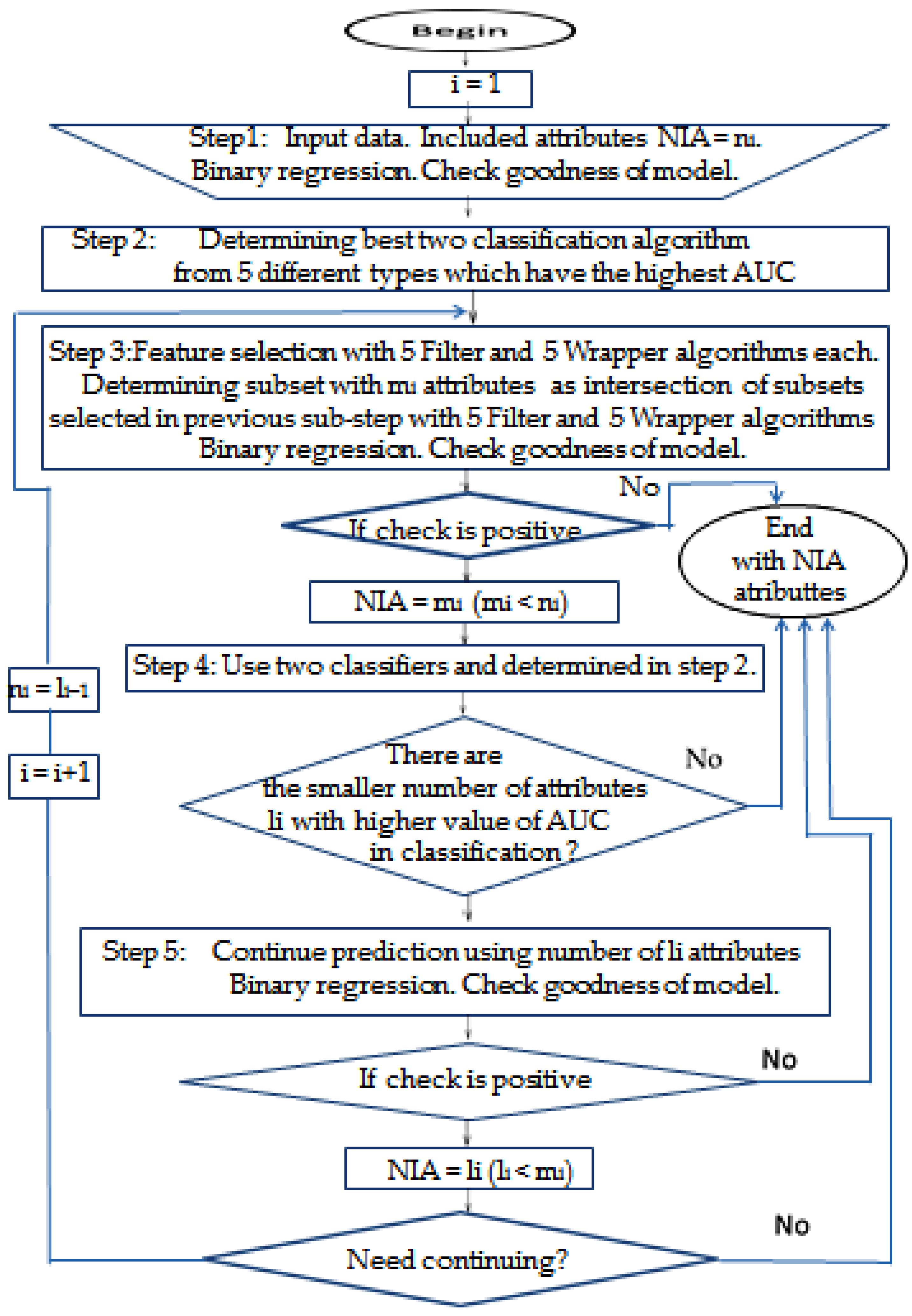
| Algorithm 1: Obtaining significant predictors of TI caused by atmospheric factors |
| 1. Perform a logistic-binary regression Enter method for a model in which n atmospheric factors are predictors and the dependent variable is the number of TI logically determined by a threshold, which could be a value greater than 150% of the average value of daily TI for considered case study, and has a nominal value 1 in that case and 0 in all others. We start the algorithm in first cycle i = 1 with referent value which represents the number of attributes which is in start step number noted as n1–in concrete case study n1 = 27. In the Enter method of binary regression used, all of the predictors will be included in the prediction; only in the possible presence of impermissible collinearity of certain predictors, they will be excluded from the model. After that, using the Cox and Snell R Square and Nagelkerke R Square test, the algorithm will determine the value of the percentage of the variance that is explained, i.e., the connection between the tested factors and the dependent variable, and using the Hosmer and Lemeshow tests, the algorithm will determine its goodness-of-fit, i.e., the adaptation of the model to the given data, i.e., calibration which will evaluate the goodness of the proposed ensemble model in this and in the later steps, including the most important last step of the proposed algorithm in order to use the AUC to determine the quality measure of the classification binary regression analysis model. 2. Apply a set of at least five methods of classification which belong to different types of classification (for example, how it is already mentioned in Weka software, so any five, each from different types—Decision trees, Bayes, Meta, Rules, Functions, MI, etc.) and find two classification algorithms from this set that has the highest value of AUC among other algorithms used (also other parameters such as precision, recall, and F-measure which are with good values). That classification algorithm will be used in the step that follows in which attribute selection is carried out to select the best of several used attribute selection algorithms from two different types of groups. The values of Hosmer and Lemeshow test and even more significant AUC values that determine the threshold of whether the desired level of goodness of the model has been reached—take the values determined in steps 1, i.e., step 2 of this algorithm, respectively. 3. Using five algorithms from each of both groups of feature selection methods is with the basic aim to use in this ensemble classification algorithms that are good and eliminate bad characteristics: 3.1. Using at least five of the mentioned attribute selection algorithms from both the wrapper and the filter groups more broadly explained in Section 2.1.3. of this paper, perform attribute classification in one class of the two possible classes of instances which are defined in step 1 of this algorithm and according to the criterion of whether the value of this attribute exceeds or does not exceed the daily TI threshold. 3.1.1. Classifiers for filter attribute selection could be any five different algorithms: for example Information-Gain Attribute evaluation, Gain-Ratio Attribute evaluation, Symmetrical Uncertainty Attribute evaluation, Chi-Square Attribute evaluation, Filtered Attribute Eval, Relief Attribute, Principal Components, etc. The authors used the first five of these in this paper. Those chosen algorithms are used to determine the feature subset of attribute A′ = {…, ai–1, ai} and their ranks from the starting set A = {a1, a2, …, an}, i ≤ n. It is necessary to remark that n is the starting number of attributes in such a way that the decision to exclude a particular attribute is made by the majority of exclusion decisions made individually by each of the algorithms. 3.1.2. Classifiers for wrapper attribute selection can be any five from this group of algorithms: for example Best First, Linear Forward Selection, Genetic Search, Greedy Stepwise, Subset Size Forward Selection, etc. The authors used the first five of these in this paper. Those chosen algorithms are used to compute a subset A″ = {…, aj–1, aj} from the starting set A = {a1, a2, …, an}, j ≤ n. It is necessary to remark that n is the starting number of attributes in such a way that the decision to exclude a particular attribute is made by the majority of exclusion decisions made individually by each of the algorithms. 3.2. Determine a subset A‴ = A′ ∩ A″ = {…, am–1, am} from the starting set A = {a1, a2, …, an}, m ≤ i, j, n, where n is the starting number of attributes and i and j values determined in the previous steps of the algorithm 3.1.1 and 3.1.2 We could have, at the end of this step, not only a different number of selected attributes using both groups of attribute selection algorithms considered as it is given in 3.1.1. and 3.1.2., possibly different notated attributes as well, and that is why we use the intersection operation for these obtained subsets A′ and A″, which determines only common attributes as those that will be removed from the initial, i.e., in later cycles from the observed set A. 3.3. If m<n exists, which is determined in the previous step 3.2., and Hosmer and Lemeshow test determined the goodness of the algorithm as positive, the algorithm continues with the next step 4 using set A‴ = {…, am–1, am} attributes; otherwise, finish with the prediction which determined the existing number of parameters which was in the observed set. 4. Choose one from five filter classifiers with the smallest number of attributes which has the highest AUC value using for that already determined two classification algorithms in step 2 of this algorithm. 5. Perform the binary regression Enter method again now with a smaller number of attributes li selected in step 4 of this algorithm, and if the values of Hosmer and Lemeshow tests are worse than those obtained in the previous test executed in step 3 of this algorithm or the obtained number of attributes satisfied value preset in advance, the procedure is finished; otherwise the procedure continues cyclically with step 3 of this algorithm with new set referent value. Preset value of the number of selected attributes on the specific need for each case separately and for the case study in this paper, the authors chose it at less than 15% from the starting number of attributes. |
2.2. Materials
3. Results and Findings
3.1. Application of Proposed Algorithm of Ensemble Learning
3.1.1. Filter
- (1)
- Information-Gain Attribute evaluation(IG),
- (2)
- Gain-Ratio Attribute evaluation (GR),
- (3)
- SymmetricalUncertAttributeEval (SU),
- (4)
- Chi-Square Attribute evaluation (CS),
- (5)
- Filtered Attribute Eval (FA).
3.1.2. Wrapper
- (1)
- Best First (BF),
- (2)
- Linear Forward Selection (LF),
- (3)
- Genetic Search (GS),
- (4)
- Greedy Stepwise (GST),
- (5)
- Subset Size Forward Selection (SSFS).
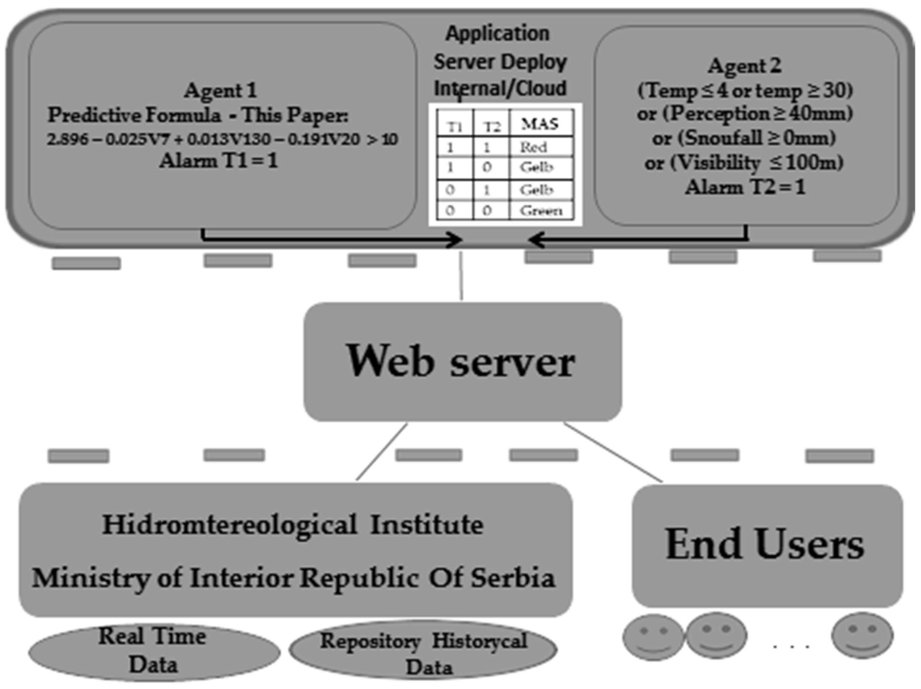
3.2. The Model of Emergent Intelligence as One Implementation of the Proposed Ensemble Method
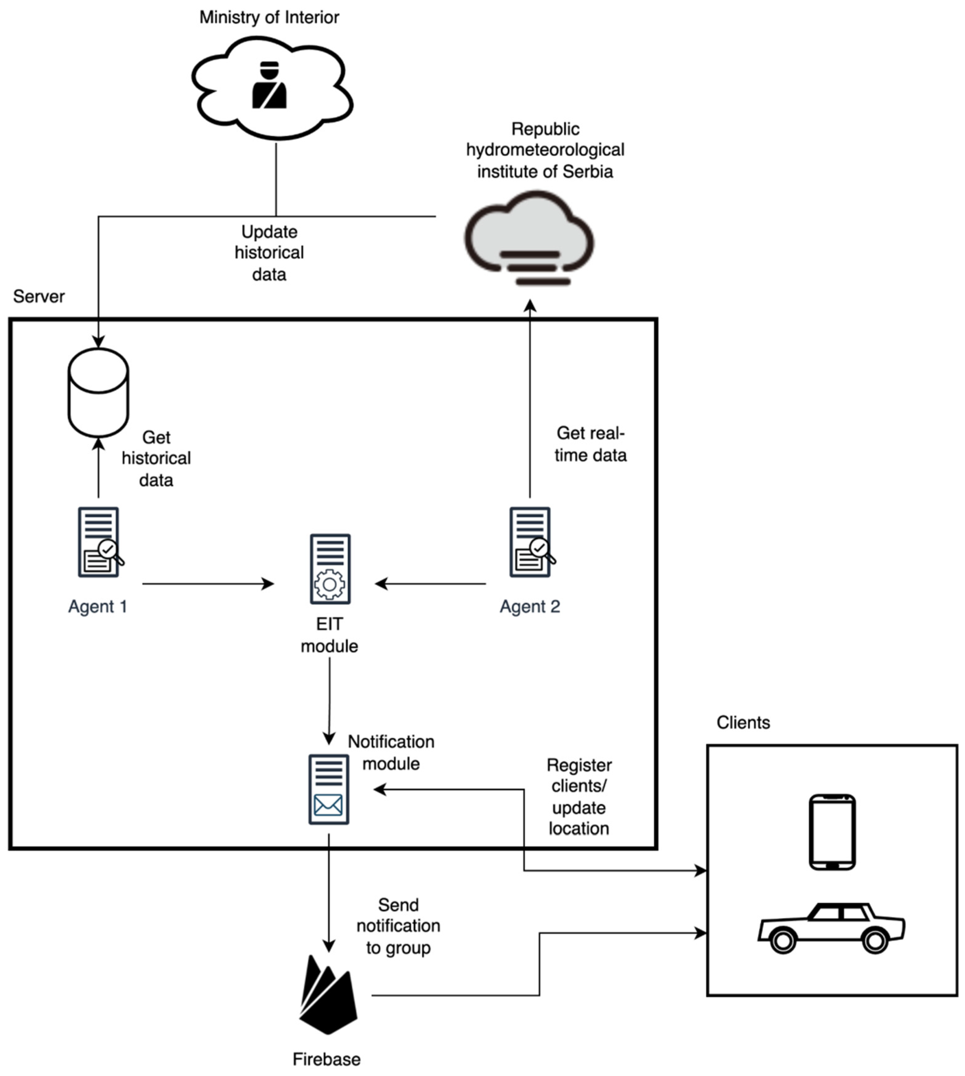
4. Technological Implementation of the Proposed Ensemble Model
4.1. The Architecture of the Proposed Technical Solution
4.2. The Implementation of Proposed Technical Solution
| Algorithm 2: Implementation of the EIT algorithm that generates alarm EITalarm |
| T1 and T 2 agent alarms |
| f (T1 = 1 and T2 = 1) |
| Red alarm |
| else |
| if (T1 = 1 or T2 = 1) |
| Yellow alarm |
| else |
| Green alarm-no alarm |
5. Conclusions
Supplementary Materials
Author Contributions
Funding
Data Availability Statement
Acknowledgments
Conflicts of Interest
References
- Gao, J.; Chen, X.; Woodward, A.; Liu, X.; Wu, H.; Lu, Y.; Li, L.; Liu, Q. The association between meteorological factors and road traffic injuries: A case analysis from Shantou city, China. Sci. Rep. 2016, 6, 37300. [Google Scholar] [CrossRef]
- Verster, T.; Fourie, E. The good, the bad and the ugly of South African fatal road accidents. S. Afr. J. Sci. 2018, 114. [Google Scholar] [CrossRef] [PubMed] [Green Version]
- Lankarani, K.B.; Heydari, S.T.; Aghabeigi, M.R.; Moafian, G.; Hoseinzadeh, A.; Vossoughi, M.J. The impact of environmental factors on traffic accidents in Iran. Inj Violence Res. 2014, 6, 64–71. [Google Scholar] [CrossRef] [Green Version]
- Dastoorpoor, M.; Idani, E.; Khanjani, N.; Goudarzi, G.; Bahrampour, A. Relationship Between Air Pollution, Weather, Traffic, and Traffic-Related Mortality. Trauma Mon. 2016, 21, e37585. [Google Scholar] [CrossRef] [Green Version]
- Chekijian, S.; Paul, M.; Kohl, V.P.; Walker, D.M.; Tomassoni, A.J.; Cone, D.C.; Vaca, F.E. The global burden of road injury: Its relevance to the emergency physician. Emerg. Med. Int. 2014, 2014, 139219. [Google Scholar] [CrossRef] [PubMed] [Green Version]
- Xie, S.H.; Wu, Y.S.; Liu, X.J.; Fu, Y.B.; Li, S.S.; Ma, H.W.; Zou, F.; Cheng, J.Q. Mortality from road traffic accidents in a rapidly urbanizing Chinese city: A 20-year analysis in Shenzhen, 1994–2013. Traffic Inj. Prev. 2016, 17, 3943. [Google Scholar] [CrossRef]
- Chan, C.T.; Pai, C.W.; Wu, C.C.; Hsu, J.C.; Chen, R.J.; Chiu, W.T.; Lam, C. Association of Air Pollution and Wheather Factors with Traffic Injuri Severity: A Study in Taiwan. Int. J. Environ. Res. Public Health 2022, 19, 7442. [Google Scholar] [CrossRef] [PubMed]
- Jalilian, M.M.; Safarpour, H.; Bazyar, J.; Keykaleh, M.S.; Malekyan, L.; Khorshidi, A. Environmental Related Risk Factors to Road Traffic Accidents in Ilam, Iran. Med. Arch. 2019, 73, 169–172. [Google Scholar] [CrossRef]
- Guyon, I.; Elisseeff, A. An Introduction to Variable and Feature Selection. J. Mach. Learn. Res. 2003, 3, 1157–1182. [Google Scholar]
- Lu, H.; Zhu, Y.; Shi, K.; Yisheng, L.; Shi, P.; Niu, Z. Using Adverse Weather Data in Social Media to Assist with City-Level Traffic Situation Awareness and Alerting. Appl. Sci. 2018, 8, 1193. [Google Scholar] [CrossRef] [Green Version]
- Trenchevski, A.; Kalendar, M.; Gjoreski, H.; Efnusheva, D. Prediction of Air Pollution Concentration Using Weather Data and Regression Models. In Proceedings of the 8th International Conference on Applied Innovations in IT, (ICAIIT), Koethen (Anhalt), Germany, 9 March 2020; pp. 55–61. [Google Scholar]
- Gupta, A.; Sharma, A.; Goel, A. Review of Regression Analysis Models. Int. J. Eng. Res. Technol. 2017, 6, 58–61. [Google Scholar]
- Theofilatos, A.; Yannis, G. A review of the effect of traffic and weather characteristics on road safety. Accid. Anal. Prev. 2014, 72, 244–256. [Google Scholar] [CrossRef]
- Qiu, L.; Nixon, W.A. Effects of adverse weather on traffic crashes: Systematic review and meta-analysis. Transp. Res. Rec. 2008, 2055, 139–146. [Google Scholar] [CrossRef]
- Edwards, J.B. The relationship between road accident severity and recorded weather. J. Saf. Res. 1998, 29, 249–262. [Google Scholar] [CrossRef]
- Malin, F.; Norros, I.; Innamaa, S. Accident risk of road and weather conditions on different road types. Accid. Anal. Prev. 2019, 122, 181–188. [Google Scholar] [CrossRef] [PubMed]
- Brijs, T.; Offermans, C.; Hermans, E.; Stiers, T. The Impact of Weather Conditions on Road Safety Investigated on an HourlyBasis. In Proceedings of the Transportation Research Board 85th Annual Meeting, Washington, DC, USA, 22–26 January 2006. [Google Scholar]
- Antoniou, C.; Yannis, G.; Katsochis, D. Impact of meteorological factors on the number of injury accidents. In Proceedings of the 13th World Conference on Transport Research (WCTR 2013), Rio de Janeiro, Brazylia, 15–18 July 2013; Volume 15. [Google Scholar]
- El-Basyouny, K.; Barua, S.; Islam, M.T. Investigation of time and weather effects on crash types using full Bayesian multivariate Poisson lognormal models. Accid. Anal. Prev. 2014, 73, 91–99. [Google Scholar] [CrossRef]
- Baker, C.; Reynolds, S. Wind-induced accidents of road vehicles. Accid. Anal. Prev. 1992, 24, 559–575. [Google Scholar] [CrossRef]
- Naik, B.; Tung, L.W.; Zhao, S.; Khattak, A.J. Weather impacts on single-vehicle truck crash injury severity. J. Saf. Res. 2016, 58, 57–65. [Google Scholar] [CrossRef] [PubMed]
- Mitra, S. Sun glare and road safety: An empirical investigation of intersection crashes. Saf. Sci. 2014, 70, 246–254. [Google Scholar] [CrossRef]
- Hagita, K.; Mori, K. The effect of sun glare on traffic accidents in Chiba prefecture, Japan. Asian Transp. Stud. 2014, 3, 205–219. [Google Scholar] [CrossRef]
- Buisán, S.T.; Earle, M.E.; Collado, J.L.; Kochendorfer, J.; Alastrué, J.; Wolff, M.; Smith, C.D.; López-Moreno, J.I. Assessment of snowfall accumulation underestimation by tipping bucket gauges in the Spanish operational network. Atmos. Meas. Tech. 2017, 10, 1079–1091. [Google Scholar] [CrossRef] [Green Version]
- Lio, C.F.; Cheong, H.H.; Un, C.H.; Lo, I.L.; Tsai, S.Y. The association between meteorological variables and road traffic injuries: A study from Macao. PeerJ 2019, 7, e6438. [Google Scholar] [CrossRef] [PubMed]
- Khan, G.; Qin, X.; Noyce, D. Spatial Analysis of Weather Crash Patterns. J. Transp. Eng. 2008, 134, 191–202. [Google Scholar] [CrossRef]
- Becker, N.; Rust, H.W.; Ulbrich, U. Predictive modeling of hourly probabilities for weather-related road accidents. Nat. Hazards Earth Syst. Sci. 2020, 20, 2857–2871. [Google Scholar] [CrossRef]
- Song, X.; Zhao, X.; Zhang, Y.; Li, Y.; Yin, C.; Chen, J. The effect of meteorological factors on road traffic injuries in Beijing. Appl. Ecol. Environ. Res. 2019, 17, 9505–9514. [Google Scholar] [CrossRef]
- Matthew, G.K.; Yannis, G. Weather Effects on Daily Traffic Accidents and Fatalities: Time Series Count Data Approach. In Proceedings of the Transportation Research Board 89th Annual Meeting, Washington, DC, USA, 10–14 January 2010; p. 17. [Google Scholar]
- Bergel-Hayat, R.; Depire, A. Climate, road traffic and road risk—An aggregate approach. In Proceedings of the 10th WCTR (World Conference on Transport Research Society), Istanbul, Turkey, 4–8 July 2004. [Google Scholar]
- Bergel-Hayat, R.; Debbarh, M.; Antoniou, C.; Yannis, G. Explaining the road accident risk: Weather effects. Accid. Anal. Prev. 2013, 60, 456–465. [Google Scholar] [CrossRef] [Green Version]
- Zheng, L.; Lin, R.; Wang, X.; Chen, W. The Development and Application of Machine Learning in Atmospheric Environment Studies. Remote Sens. 2021, 13, 4839. [Google Scholar] [CrossRef]
- Yuan, Q.; Shen, H.; Li, T.; Li, Z.; Li, S.; Jiang, Y.; Xu, H.; Tan, W.; Yang, Q.; Wang, J. Deep learning in environmental remote sensing: Achievements and challenges. Remote Sens. Environ. 2020, 241, 111716. [Google Scholar] [CrossRef]
- Medina-Salgado, B.; Sánchez-DelaCruz, E.; Pozos-Parra, P.; Sierra, J.E. Urban traffic flow prediction techniques: A review. Sustain. Comput. Inform. Syst. 2022, 35, 100739. [Google Scholar] [CrossRef]
- Shaik, M.E.; Islam, M.M.; Hossain, Q.S. A review on neural network techniques for the prediction of road traffic accident severity. Asian Transp. Stud. 2021, 7, 100040. [Google Scholar] [CrossRef]
- Moghaddam, F.R.; Afandizadeh, S.; Ziyadi, M. Prediction of accident severity using artificial neural networks. Int. J. Civ. Eng. 2011, 9, 41–49. [Google Scholar]
- Pradhan, B.; Sameen, M.I. Review of traffic accident predictions with neural networks. In Laser Scanning Systems in Highway and Safety Assessment, Technology & Innovation (IEREK Interdisciplinary Series for Sustainable Development); Springer: Cham, Switzerland, 2020; pp. 97–109. [Google Scholar]
- Profillidis, V.A.; Botzoris, G.N. Chapter 8—Artificial intelligence—Neural network methods. In Modeling of Transport Demand Analyzing, Calculating, and Forecasting Transport Demand; Elsevier: St. Louis, MO, USA, 2019; pp. 353–382. [Google Scholar] [CrossRef]
- Yuan, J.; Abdel-Aty, M.; Gong, Y.; Cai, Q. Real-time crash risk prediction using long short-term memory recurrent neural network. Transport. Res. Rec. J. Transport. Res. Board 2019, 2673, 1–13. [Google Scholar] [CrossRef]
- Rezapour, M.; Nazneen, S.; Ksaibati, K. Application of deep learning techniques in predicting motorcycle crash severity. Eng. Rep. 2020, 2, e12175. [Google Scholar] [CrossRef]
- Sameen, M.I.; Pradhan, B.; Shafri, H.Z.M.; Hamid, H.B. Applications of deep learning in severity prediction of traffic accidents. In Global Civil Engineering Conference; Springer: Singapore, 2019; pp. 793–808. [Google Scholar]
- Zheng, M.; Li, T.; Zhu, R.; Chen, J.; Ma, Z.; Tang, M.; Cui, Z.; Wang, A.Z. Traffic accident’s severity prediction: A deep-learning approach-based CNN network. IEEE Access 2019, 7, 39897–39910. [Google Scholar] [CrossRef]
- Sameen, M.I.; Pradhan, B. Severity prediction of traffic accidents with recurrent neural networks. Appl. Sci. 2017, 7, 476. [Google Scholar] [CrossRef] [Green Version]
- Soto, B.G.; Bumbacher, A.; Deublein, M.; Adey, B.T. Predicting road traffic accidents using artificial neural network models. Infrastruct. Asset Manag. 2018, 5, 132–144. [Google Scholar] [CrossRef] [Green Version]
- Ebrahim, S.; Hossain, Q.S. An Artificial Neural Network Model for Road Accident Prediction: A Case Study of Khulna Metropolitan City, Bangladesh. In Proceedings of the Fourth International Conference on Civil Engineering for Sustainable Development (ICCESD 2018), Khulna, Bangladesh, 9–11 February 2018; KUET: Khulna, Bangladesh, 2018. [Google Scholar]
- Jadaan, K.S.; Al-Fayyad, M.; Gammoh, H.F. Prediction of road traffic accidents in Jordan using artificial neural network (ANN). J. Traffic Log. Eng. 2014, 2, 92–94. [Google Scholar] [CrossRef] [Green Version]
- Moslehi, S.; Gholami, A.; Haghdoust, Z.; Abed, H.; Mohammadpour, S.; Moslehi, M.A. Predictions of traffic accidents based on wheather coditions in Gilan provice using artificial neuran network. J. Health Adm. 2021, 24, 67–78. [Google Scholar]
- Liu, Y. Weather Impact on Road Accident Severity in Maryland. Ph.D. Thesis, Faculty of Graduate School, Maryland University, College Park, MD, USA, 2013. [Google Scholar]
- Zou, X. Bayesian network approach to causation analysis of road accidents using Netica. J. Adv. Transp. 2017, 2017, 2525481. [Google Scholar] [CrossRef] [Green Version]
- Ogwueleka, F.N.; Misra, S.; Ogwueleka, T.C.; Fernandez-Sanz, L. An artificial neural network model for road accident prediction: A case study of a developing country. Acta Polytech. Hung. 2014, 11, 177–197. [Google Scholar]
- Kunt, M.M.; Aghayan, I.; Noii, N. Prediction for traffic accident severity: Comparing the artificial neural network, genetic algorithm, combined genetic algorithm and pattern search methods. Transport 2011, 26, 353–366. [Google Scholar] [CrossRef] [Green Version]
- Taamneh, M.; Taamneh, S.; Alkheder, S. Clustering-based classification of road traffic accidents using hierarchical clustering and artificial neural networks. Int. J. Inj. Control Saf. Promot. 2017, 24, 388–395. [Google Scholar] [CrossRef]
- Ghasedi, M.; Sarfjoo, M.; Bargegol, I. Prediction and Analysis of the Severity and Number of Suburban Accidents Using Logit Model, Factor Analysis and Machine Learning: A case study in a developing country. SN Appl. Sci. 2021, 3, 13. [Google Scholar] [CrossRef]
- Mondal, A.R.; Bhuiyan, M.A.; Yang, F. Advancement of weather-related crash prediction model using nonparametric machine learning algorithms. SN Appl. Sci. 2020, 2, 1372. [Google Scholar] [CrossRef]
- Liang, M.; Zhang, Y.; Yao, Z.; Qu, G.; Shi, T.; Min, M.; Ye, P.; Duan, L.; Bi, P.; Sun, Y. Meteorological Variables and Prediction of Road Traffic Accident Severity in Suzhou city of Anhui Province of China. 2020. Available online: https://www.researchgate.net/publication/340197416MeteorologicalVariables_and_Prediction____Road_Traffic_Accident_Severity_in_Suzhou_city_of_Anhui_Province_of_China (accessed on 20 November 2022). [CrossRef]
- Olutayo, V.A.; Eludire, A.A. Traffic accident analysis using decision trees and neural networks. Int. J. Inf. Technol. Comput. Sci. 2014, 6, 22–28. [Google Scholar]
- Silva, H.C.E.; Saraee, M.H. Predicting road traffic accident severity using decision trees and time-series calendar heat maps. In Proceedings of the 6th IEEE Conference on Sustainbility Utilization and Development in Engineering and Technology, Penang, Malaysia, 7–9 November 2019. [Google Scholar]
- Chong, M.; Abraham, A.; Paprzycki, M. Traffic Accident Analysis Using Decision Trees and Neural Networks. arXiv 2004, arXiv:cs/0405050. [Google Scholar]
- Bahiru, T.K.; Kumar Singh, D.; Tessfaw, E.A. Comparative study on Data Mining Classification Algorithms for Predicting Road Traffic Accident Severity. In Proceedings of the 2018 Second Inernational Conference on Inventive Communication and Computational Technologies ICICCT, Coimbatore, India, 20–21 April 2018; pp. 1655–1660. [Google Scholar] [CrossRef]
- Al-Turaiki, I.; Aloumi, M.; Aloumi, N.; Alghamdi, K. Modeling traffic accidents in Saudi Arabia using classification techniques. In Proceedings of the 2016 4th Saudi International Conference on Information Technology (Big data aNALYSIS) KACSTIT, Ryadh, Saudi Arabia, 6–9 November 2016; pp. 1–5. [Google Scholar] [CrossRef]
- Lepperod, A.J. Air Quality Prediction with Machine Learning. Master’s Thesis, Norwegian University of Science and Technology, Oslo, Norway, 2019. [Google Scholar]
- Dong, S.; Khattak, A.; Ullah, I.; Zhou, J.; Hussain, A. Predicting and Analyzing Road Traffic Injury Severity Using Boosting-Based Ensemble Learning Models with SHAPley Additive exPlanations. Int. J. Environ. Res. Public Health 2022, 19, 2925. [Google Scholar] [CrossRef] [PubMed]
- Kim, J.H.; Kim, J.; Lee, G.; Park, J. Machine Learning-Based Models for Accident Prediction at a Korean Container Port. Sustainability 2021, 13, 9137. [Google Scholar] [CrossRef]
- Gutierrez-Osorio, C.; González, F.A.; Pedraza, C.A. Deep Learning Ensemble Model for the Prediction of Traffic Accidents Using Social Media Data. Computers 2022, 11, 126. [Google Scholar] [CrossRef]
- Yuexu, Z.; Wei, D. Prediction in Traffic Accident Duration Based on Heterogeneous Ensemble Learning. Appl. Artif. Intell. 2022, 36, 2018643. [Google Scholar] [CrossRef]
- Chang, L.Y.; Wang, H.W. Analysis of traffic injury severity: An application of non-parametric classification tree techniques. Accid. Anal. Prev. 2006, 38, 1019–1027. [Google Scholar] [CrossRef] [PubMed]
- Yang, G.; Wang, Y.; Yu, H.; Ren, Y.; Xie, J. Short-Term Traffic State Prediction Based on the Spatiotemporal Features of Critical Road Sections. Sensors 2018, 18, 2287. [Google Scholar] [CrossRef] [Green Version]
- Li, G.; Knoop, V.L.; Van Lint, H. Estimate the limit of predictability in short-term traffic forecasting: An entropy-based approach. Transp. Res. Part C Emerg. Technol. 2022, 138, 103607. [Google Scholar] [CrossRef]
- Min, W.; Wynter, L. Real-time road traffic prediction with spatio-temporal correlations. Transp. Res. Part C Emerg. Technol. 2011, 19, 606–616. [Google Scholar] [CrossRef]
- Paz, A.; Veeramisti, N.; De la Fuente-Mella, H. Forecasting Performance Measures for Traffic Safety Using Deterministic and Stochastic Models. In Proceedings of the IEEE 18th International Conference on Intelligent Transportation Systems, Gran Canaria, Spain, 15–18 September 2015; pp. 2965–2970. [Google Scholar] [CrossRef] [Green Version]
- Pang, Y.; Zhao, X.; Yan, H.; Liu, Y. Data-driven trajectory prediction with weather uncertainties: A bayesian deep learning approach. Transp. Res. Part C Emerg. Technol. 2021, 130, 103326. [Google Scholar] [CrossRef]
- Pang, Y.; Zhao, X.; Hu, J.; Yan, H.; Liu, Y. Bayesian spatio-temporal graph transformer network(b-star) for multi-aircraft trajectory prediction. Knowl. Based Syst. 2022, 249, 108998. [Google Scholar] [CrossRef]
- Pang, Y.; Guo, Z.; Zhuang, B. Prospectnet: Weighted conditional attention for future interaction modeling in behavior prediction. arXiv 2022, arXiv:2208.13848. [Google Scholar]
- Romero, C.; Ventura, S.; Espejo, P.; Hervas, C. Data mining algorithms to classify students. Proceedings for the 1st IC on Educational Data Mining (EDM08), Montreal, QC, Canada, 20–21 June 2008; pp. 20–21. [Google Scholar]
- Fawcett, T. ROC Graphs: Notes and Practical Considerations for Data Mining Researchers; Technical Report HP Laboratories: Palo Alto, CA, USA, 2003. [Google Scholar]
- Vuk, M.; Curk, T. ROC curve, lift chart and calibration plot. Metod. Zv. 2006, 3, 89–108. [Google Scholar] [CrossRef]
- Dimić, G.; Prokin, D.; Kuk, K.; Micalović, M. Primena Decision Trees i Naive Bayes klasifikatora na skup podataka izdvojen iz Moodle kursa. In Proceedings of the Conference INFOTEH, Jahorina, Bosnia and Herzegovina, 21–23 March 2012; Volume 11, pp. 877–882. [Google Scholar]
- Witten, H.; Eibe, F. Data Mining: Practical Machine Learning Tools and Techniques, 2nd ed.; Morgan Kaufmann Series in Data Management Systems; Elsevier: Cambridge, MA, USA, 2005. [Google Scholar]
- Benoit, G. Data Mining. Annu. Rev. Inf. Sci. Technol. 2002, 36, 265–310. [Google Scholar] [CrossRef]
- Weka (University of Waikato: New Zealand). Available online: http://www.cs.waikato.ac.nz/ml/weka (accessed on 20 November 2022).
- Berrar, D. Bayes’ Theorem and Naive Bayes Classifier. Encycl. Bioinform. Comput. Biol. 2018, 1, 403–412. [Google Scholar] [CrossRef]
- Zhang, H. The Optimality of Naive Bayes, FLAIRS Conference; AAAI Press: Miami Beach, FL, USA, 2004. [Google Scholar]
- Friedman, J.; Hastie, T.; Tibshirani, R. Additive Logistic Regression: A Statistical View of Boosting. Ann. Stat. 2000, 28, 337–407. [Google Scholar] [CrossRef]
- Rokach, L.; Maimon, O. Decision Trees. In The Data Mining and Knowledge Discovery Handbook; Springer: Boston, MA, USA, 2005; pp. 165–192. [Google Scholar] [CrossRef]
- Xiaohu, W.; Lele, W.; Nianfeng, L. An Application of Decision Tree Based on ID3. Phys. Procedia 2012, 25, 1017–1021. [Google Scholar] [CrossRef]
- Quinlan, J.R. C4.5: Programs for Machine Learning; Morgan Kaufmann: San Mateo, CA, USA, 1993. [Google Scholar]
- Bella, A.; Ferri, C.; Hernández-Orallo, J.; Ramírez-Quintana, M.J. Calibration of machine learning models. In Handbook of Research on Machine Learning Applications; IGI Global: Hershey, PA, USA, 2009. [Google Scholar]
- SPSS Statistics 17.0 Brief Guide. Available online: http://www.sussex.ac.uk/its/pdfs/SPSS_Statistics_Brief_Guide_17.0.pdf (accessed on 20 November 2022).
- Liu, H.; Motoda, H. Feature Selection for Knowledge Discovery and Data Mining; Kluwer Academic: Boston, MA, USA, 1998. [Google Scholar]
- Dash, M.; Liu, H.; Motoda, H. Consistency based feature selection. In Proceedings of the Fourth Pacific Asia Conference on Knowledge Discovery and Data Mining, Kyoto, Japan, 18–20 April 2000; pp. 98–109. [Google Scholar]
- Hall, M.A. Correlation-Based Feature Selection for Discrete and Numeric Class Machine Learning. In Proceedings of the 17th IEEE Int’l Conf. Machine Learning, Orlando, FL, USA, 17–20 December 2000; pp. 359–366. [Google Scholar]
- Novaković, J. Rešavanje klasifikacionih problema mašinskog učenja. In Bussines Process Reeingineering; Faculty of Technical sciences Čačak, University of Kragujevac: Kragujevac, Serbia, 2013; Volume 4. [Google Scholar]
- Daelemans, W.; Hoste, V.; Meulder, F.D.; Naudts, B. Combined Optimization of Feature Selection and Algorithm Parameter Interaction in Machine Learning of Language. In Proceedings of the 14th European Conference on Machine Learning (ECML-2003), Lecture Notes in Computer Science 2837, Cavtat-Dubrovnik, Croatia, 22–26 September 2003; pp. 84–95. [Google Scholar]
- Hall, M.A.; Smith, L.A. Practical feature subset selection for machine learning. In Proceedings of the 21st Australian Computer Science Conference, Perth, Australia, 4–6 February 1998; pp. 181–191. [Google Scholar]
- Moriwal, R.; Prakash, V. An efficient info-gain algorithm for finding frequent sequential traversal patterns from web logs based on dynamic weight constraint. In Proceedings of the CUBE International Information Technology Conference (CUBE ’12), Pune, India, 3– 6September 2012; ACM: New York, NY, USA, 2012; pp. 718–723. [Google Scholar]
- Salzberg, L.S. Book Review: C4.5: By J. Ross Quinlan. Inc., 1993. Programs for Machine Learning Morgan Kaufmann Publishers. Mach. Learn. 1994, 16, 235–240. [Google Scholar] [CrossRef] [Green Version]
- Thakur, D.; Markandaiah, N.; Raj, D.S. Re optimization of ID3 and C4.5 decision tree. In Proceedings of the 2010 International Conference on Computer and Communication Technology (ICCCT 2010), Allahabad, Uttar Pradesh, India, 17–19 September 2010; pp. 448–450. [Google Scholar]
- Available online: https://www.programiz.com/dsa/greedy-algorithm (accessed on 15 November 2022).
- Girish, S.; Chandrashekar, F. A survey on feature selection methods. Comput. Electr. Eng. 2014, 40, 16–28. [Google Scholar]
- Moore, S.; Notz, I.; Flinger, A. The Basic Practice of Statistics; W.H. Freeman: New York, NY, USA, 2013. [Google Scholar]
- Ilin, V. The Models for Identification and Quantification of the Determinants of ICT Adoption in Logistics Enterprises. Ph.D. Thesis, Faculty of Technical Sciences University Novi Sad, Novi Sad, Serbia, 2018. [Google Scholar]
- Hair, J.F.; Anderson, R.E.; Tatham, R.L.; Black, W.C. Multivariate Data Analysis; Prentice-Hall, Inc.: New York, NY, USA, 1998. [Google Scholar]
- Yang, T.; Ying, Y. AUC Maximization in the Era of Big Data and AI: A Survey. ACM Comput. Surv. 2022, 37. [Google Scholar] [CrossRef]


| Predicted Label | |||
|---|---|---|---|
| Positive | Negative | ||
| Actual label | Positive | TP(true positive) | FN(false negative) |
| Negative | FP(false positive) | TN(true negative) | |
| Variable | Parameter |
|---|---|
| 1-V1 | Air pressure at 7 o’clock (mbar) |
| 2-V2 | Air pressure at 14 o’clock (mbar) |
| 3-V3 | Air pressure at 21 o’clock (mbar) |
| 4-V4 | Mean daily air pressure (mbar) |
| 5-V5 | Maximum daily temperature (°C) |
| 6-V6 | Minimum daily temperature (°C) |
| 7-V7 | Daily temperature amplitude (°C) |
| 8-V8 | Temperature at 7 o’clock (°C) |
| 9-V9 | Temperature at 14 o’clock (°C) |
| 10-V10 | Temperature at 21 o’clock (°C) |
| 11-V11 | Mean daily temperature (°C) |
| 12-V12 | Relative humidity at 7 o’clock -percent |
| 13-V13 | Relative humidity at 14 o’clock -percent |
| 14-V14 | Relative humidity at 21 o’clock -percent |
| 15-V15 | Mean daily relative humidity-percent |
| 16-V16 | Water vapour saturation at 7 o’clock (mbar) |
| 17-V17 | Water vapour saturation at 14 o’clock (mbar) |
| 18-V18 | Water vapour saturation at 21 o’clock (mbar) |
| 19-V19 | Mean daily water vapour saturation (mbar) |
| 20-V20 | Mean daily wind speed (m/sec) |
| 21-V21 | Insolation (h) |
| 22-V22 | Cloudiness at 7 o’clock (in tenths of the sky) |
| 23-V23 | Cloudiness at 14 o’clock (in tenths of the sky) |
| 24-V24 | Cloudiness at 21 o’clock (in tenths of the sky) |
| 25-V25 | Mean daily cloudiness (in tenths of the sky) |
| 26-V26 | Snowfall (cm) |
| 27-V27 | Rainfall (mm) |
| 28-V28 | Number of daily traffic accidents |
| Binary Regression | |||||||||
|---|---|---|---|---|---|---|---|---|---|
| B | S.E. | Wald | Df | Sig. | Exp (B) | ||||
| 1-V1 | −0.076 | 0.061 | 1.583 | 1 | 0.208 | 0.927 | |||
| 2-V2 | −0.057 | 0.073 | 0.610 | 1 | 0.435 | 0.945 | |||
| 3-V3 | −0.129 | 0.061 | 4.508 | 1 | 0.034 | 0.879 | |||
| 4-V4 | 0.265 | 0.148 | 3.199 | 1 | 0.074 | 1.303 | |||
| 5-V5 | 0.078 | 0.095 | 0.661 | 1 | 0.416 | 1.081 | |||
| 6-V6 | −0.045 | 0.097 | 0.215 | 1 | 0.643 | 0.956 | |||
| 7-V7 | −0.020 | 0.092 | 0.050 | 1 | 0.824 | 0.980 | |||
| 8-V8 | −0.018 | 0.067 | 0.077 | 1 | 0.782 | 0.982 | |||
| 9-V9 | −0.094 | 0.065 | 2.088 | 1 | 0.148 | 0.910 | |||
| 10-V10 | −0.137 | 0.085 | 2.572 | 1 | 0.109 | 0.872 | |||
| 11-V11 | 0.229 | 0.143 | 2.557 | 1 | 0.110 | 1.257 | |||
| 12-V12 | 0.083 | 0.057 | 2.072 | 1 | 0.150 | 1.086 | |||
| 13-V13 | 0.092 | 0.058 | 2.527 | 1 | 0.112 | 1.096 | |||
| 14=V14 | 0.068 | 0.058 | 1.368 | 1 | 0.242 | 1.070 | |||
| 15-V15 | −0.220 | 0.170 | 1.672 | 1 | 0.196 | 0.802 | |||
| 16-V16 | 0.018 | 0.078 | 0.053 | 1 | 0.817 | 1.018 | |||
| 17-V17 | −0.069 | 0.069 | 1.005 | 1 | 0.316 | 0.933 | |||
| 18-V18 | 0.072 | 0.082 | 0.759 | 1 | 0.384 | 1.074 | |||
| 19-V19 | −0.031 | 0.149 | 0.045 | 1 | 0.832 | 0.969 | |||
| 20-V20 | −0.162 | 0.075 | 4.640 | 1 | 0.031 | 0.850 | |||
| 21-V21 | −0.020 | 0.031 | 0.402 | 1 | 0.526 | 0.981 | |||
| 22-V22 | −0.023 | 0.064 | 0.132 | 1 | 0.716 | 0.977 | |||
| 23-V23 | −0.050 | 0.065 | 0.584 | 1 | 0.445 | 0.951 | |||
| 24-V24 | 0.028 | 0.063 | 0.194 | 1 | 0.660 | 1.028 | |||
| 25-V25 | −0.004 | 0.182 | 0.000 | 1 | 0.984 | 0.996 | |||
| Constant | 0.057 | 0.033 | 3.098 | 1 | 0.078 | 1.059 | |||
| Classification Table a,b | |||||||||
| Observed | Predicted | Percentage Correct | |||||||
| Number of daily traffic accidents > 10 | |||||||||
| 0 | 1 | ||||||||
| Step 0 | Number of daily traffic accidents > 10 | 0 | 3522 | 0 | 100.0 | ||||
| 1 | 468 | 0 | 0.0 | ||||||
| Overall Percentage | 88.3 | ||||||||
| a. Constant is included in the model. b. The cut value is 0.500. | |||||||||
| Model Summary | |||||||||
| Step | −2 Log likelihood | Cox–Snell R Square | Nagelkerke R Square | ||||||
| 1 | 2833.054 c | 0.013 | 0.025 | ||||||
| c. Estimation terminated at iteration 5 because parameter estimates changed by less than 0.001. | |||||||||
| Hosmer and Lemeshow Test. | |||||||||
| Step | Chi-square | Df | Sig. | ||||||
| 1 | 12.187 | 8 | 0.143 | ||||||
| Accuracy | Recall | F1 Measure | ROC | |
|---|---|---|---|---|
| J48 | 0.794 | 0.881 | 0.828 | 0.496 |
| Naive Bayes | 0.809 | 0.827 | 0.817 | 0.541 |
| Logit Boost | 0.779 | 0.881 | 0.827 | 0.547 |
| PART | 0.815 | 0.882 | 0.829 | 0.524 |
| SMO | 0.779 | 0.883 | 0.828 | 0.500 |
| SU | GR | IG | CS | FA | |
|---|---|---|---|---|---|
| 13-V13 | 1/0.0063 | 1/0.0054 | 1/0.0038 | 1/23.13 | 1/0.0038 |
| 7-V7 | 2/0.0055 | 2/0.0051 | 2/0.0031 | 2/19.29 | 2/0.0031 |
| 20-V20 | 3/0.0039 | 3/0.0034 | 4/0.0023 | 4/11.89 | 4/0.0023 |
| 15-V15 | 4/0.0038 | 4/0.0029 | 3/0.0029 | 3/16.32 | 3/0.0029 |
| 4-V4 | 5/0 | 5/0 | 5/0 | 5/0 | 5/0 |
| 10-V10 | 6/0 | 6/0 | 9/0 | 9/0 | 9/0 |
| 3-V3 | 7/0 | 7/0 | 14/0 | 14/0 | 14/0 |
| 11-V11 | 8/0 | 8/0 | 7/0 | 7/0 | 7/0 |
| 9-V9 | 9/0 | 9/0 | 8/0 | 8/0 | 8/0 |
| 8-V8 | 10/0 | 10/0 | 10/0 | 10/0 | 10/0 |
| 2-V2 | 11/0 | 11/0 | 6/0 | 6/0 | 6/0 |
| 5-V5 | 12/0 | 12/0 | 11/0 | 11/0 | 11/0 |
| 6-V6 | 13/0 | 13/0 | 12/0 | 12/0 | 12/0 |
| 12-V12 | 14/0 | 14/0 | 13/0 | 13/0 | 13/0 |
| 27-V27 | 15/0 | 15/0 | 15/0 | 15/0 | 15/0 |
| 14-V14 | 16/0 | 16/0 | 16/0 | 16/0 | 16/0 |
| 26-V26 | 17/0 | 17/0 | 17/0 | 17/0 | 17/0 |
| 24-V24 | 18/0 | 18/0 | 18/0 | 18/0 | 18/0 |
| 25-V25 | 19/0 | 19/0 | 19/0 | 19/0 | 19/0 |
| 22-V22 | 20/0 | 20/0 | 20/0 | 20/0 | 20/0 |
| 23-V23 | 21/0 | 21/0 | 21/0 | 21/0 | 21/0 |
| 21-V21 | 22/0 | 22/0 | 22/0 | 22/0 | 22/0 |
| 16-V16 | 23/0 | 23/0 | 23/0 | 23/0 | 23/0 |
| 17-V17 | 24/0 | 24/0 | 24/0 | 24/0 | 24/0 |
| 18-V18 | 25/0 | 25/0 | 25/0 | 25/0 | 25/0 |
| 19-V19 | 26/0 | 26/0 | 26/0 | 26/0 | 26/0 |
| 1-V1 | 27/0 | 27/0 | 27/0 | 27/0 | 27/0 |
| BF | LF | GS | GST | SSFS | |
|---|---|---|---|---|---|
| 7-V7 | ✓ | ✓ | ✓ | ✓ | ✓ |
| 13-V13 | ✓ | ✓ | ✓ | ✓ | ✓ |
| 20-V20 | ✓ | ✓ | ✓ | ✓ | ✓ |
| 15-V15 | ✓ | ✓ | ✓ | ✓ | ✓ |
| Binary Regression Enter Method | ||||||||
|---|---|---|---|---|---|---|---|---|
| B | S.E. | Wald | Df | Sig. | Exp (B) | |||
| V7 | 0.025 | 0.017 | 2.039 | 1 | 0.153 | 1.025 | ||
| V13 | 0.013 | 0.008 | 3.002 | 1 | 0.083 | 1.013 | ||
| V15 | 0.003 | 0.010 | 0.068 | 1 | 0.794 | 1.003 | ||
| V20 | −0.184 | 0.078 | 5.601 | 1 | 0.018 | 0.832 | ||
| Constant | 0.003 | 0.010 | 0.068 | 1 | 0.794 | 1.003 | ||
| Classification Table a,b | ||||||||
| Observed | Predicted | Percentage Correct | ||||||
| Number of daily traffic accidents > 10 | ||||||||
| 0 | 1 | |||||||
| Step 0 | Number of daily traffic accidents > 10 | 0 | 3522 | 0 | 100.0 | |||
| 1 | 468 | 0 | 0.0 | |||||
| Overall Percentage | 88.3 | |||||||
| a. Constant is included in the model. b. The cut value is 0.500. | ||||||||
| Model Summary | ||||||||
| Step | −2 Log likelihood | Cox–Snell R Square | Nagelkerke R Square | |||||
| 1 | 2860.403 c | 0.006 | 0.012 | |||||
| c. Estimation terminated at iteration number 4 because parameter estimates changed by less than 0.001. | ||||||||
| Hosmer and Lemeshow Test | ||||||||
| Step | Chi-square | Df | Sig. | |||||
| 1 | 11.234 | 8 | 0.189 | |||||
| Accuracy | Recall | F1 Measure | ROC | |
|---|---|---|---|---|
| Naive Bayes | 0.809/0.779 | 0.827/0.883 | 0.817/0.828 | 0.541/0.565 |
| Logit Boost | 0.779/0.897 | 0.881/0.883 | 0.827/0.828 | 0.547/0.610 |
| Accuracy | Recall | F1 Measure | ROC | |
|---|---|---|---|---|
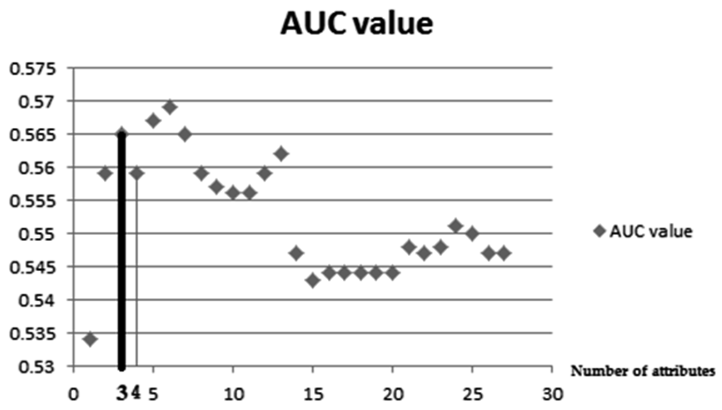
| 27 parameters | 0.779 | 0.881 | 0.827 | 0.547 |
| 4 parameters | 0.897 | 0.883 | 0.828 | 0.610 |
| 3 parameters | 0.897 | 0.883 | 0.828 | 0.613 |
| Binary Regression | |||||||||
|---|---|---|---|---|---|---|---|---|---|
| B | S.E. | Wald | Df | Sig. | Exp (B) | ||||
| V7 | 0.025 | 0.017 | 2.120 | 1 | 0.145 | 1.025 | |||
| V13 | 0.015 | 0.004 | 11.002 | 1 | 0.001 | 1.015 | |||
| V20 | −0.191 | 0.073 | 6.877 | 1 | 0.009 | 0.826 | |||
| Constant | −2.896 | 0.457 | 40.170 | 1 | 0.000 | 0.055 | |||
| Classification Table a,b | |||||||||
| Observed | Predicted | Percentage Correct | |||||||
| Number of daily traffic accidents > 10 | |||||||||
| 0 | 1 | ||||||||
| Step 0 | Number of daily traffic accidents > 10 | 0 | 3522 | 0 | 100.0 | ||||
| 1 | 468 | 0 | 0.0 | ||||||
| Overall Percentage | 88.3 | ||||||||
| a. Constant is included in the model. b. The cut value is 0.500. | |||||||||
| Model Summary | |||||||||
| Step | −2 Log likelihood | Cox–Snell R Square | Nagelkerke R Square | ||||||
| 1 | 2860.472 c | 0.006 | 0.012 | ||||||
| c. Estimation terminated at iteration number 4 because parameter estimates changed by less than 0.001. | |||||||||
| Hosmer and Lemeshow Test | |||||||||
| Step | Chi-square | Df | Sig. | ||||||
| 1 | 10.469 | 8 | 0.234 | ||||||
| T1 | T2 | EITalarm |
|---|---|---|
| 1 | 1 | Red |
| 1 | 0 | Gelb |
| 0 | 1 | Gelb |
| 0 | 0 | Green |
Disclaimer/Publisher’s Note: The statements, opinions and data contained in all publications are solely those of the individual author(s) and contributor(s) and not of MDPI and/or the editor(s). MDPI and/or the editor(s) disclaim responsibility for any injury to people or property resulting from any ideas, methods, instructions or products referred to in the content. |
© 2023 by the authors. Licensee MDPI, Basel, Switzerland. This article is an open access article distributed under the terms and conditions of the Creative Commons Attribution (CC BY) license (https://creativecommons.org/licenses/by/4.0/).
Share and Cite
Aleksić, A.; Ranđelović, M.; Ranđelović, D. Using Machine Learning in Predicting the Impact of Meteorological Parameters on Traffic Incidents. Mathematics 2023, 11, 479. https://doi.org/10.3390/math11020479
Aleksić A, Ranđelović M, Ranđelović D. Using Machine Learning in Predicting the Impact of Meteorological Parameters on Traffic Incidents. Mathematics. 2023; 11(2):479. https://doi.org/10.3390/math11020479
Chicago/Turabian StyleAleksić, Aleksandar, Milan Ranđelović, and Dragan Ranđelović. 2023. "Using Machine Learning in Predicting the Impact of Meteorological Parameters on Traffic Incidents" Mathematics 11, no. 2: 479. https://doi.org/10.3390/math11020479