Multi-Step Ahead Ex-Ante Forecasting of Air Pollutants Using Machine Learning

Abstract

In this study, a novel general multi-step ahead strategy is developed for forecasting time series of air pollutants. The values of the predictors at future moments are gathered from official weather forecast sites as independent ex-ante data. They are updated with new forecasted values every day. Each new sample is used to build- a separate single model that simultaneously predicts future pollution levels. The sought forecasts were estimated by averaging the actual predictions of the single models. The strategy was applied to three pollutants—PM₁₀, SO₂, and NO₂—in the city of Pernik, Bulgaria. Random forest (RF) and arcing (Arc-x4) machine learning algorithms were applied to the modeling. Although there are many highly changing day-to-day predictors, the proposed averaging strategy shows a promising alternative to single models. In most cases, the root mean squared errors (RMSE) of the averaging models (aRF and aAR) for the last 10 horizons are lower than those of the single models. In particular, for PM₁₀, the aRF’s RMSE is 13.1 vs. 13.8 micrograms per cubic meter for the single model; for the NO₂ model, the aRF exhibits 21.5 vs. 23.8; for SO_2, the aAR has 17.3 vs. 17.4; for NO₂, the aAR’s RMSE is 22.7 vs. 27.5, respectively. Fractional bias is within the same limits of (−0.65, 0.7) for all constructed models.

1. Introduction

Air pollution is a major and worsening environmental problem in many countries worldwide. The systematic accumulation of harmful aerosols in the air in populated areas is the cause of many diseases among their inhabitants. It leads to undesirable changes in the climate, forest, land, and all vital ecological systems [1,2]. Particulate matter, in particular, is dangerous for human health, examples include PM₁₀ (with a diameter of less than 10 microns), PM_2.5 (with a diameter of less than 2.5 microns), nitrogen dioxide (NO₂), sulfur dioxide (SO₂), ground-level ozone (O₃), and others. Numerous studies have established the harmful influence of elevated concentrations of pollutants in ambient air, leading to heart disease, acute respiratory infection, chronic obstructive pulmonary disease, allergic dysfunction, lung cancer, and more [3,4]. Even at low concentrations, the presence of a constant background of polluted air is dangerous, primarily for small children and the elderly, as well as for the chronically ill [5]. The leading causes of poor quality air in populated areas can be conditionally divided into two large groups. On the one hand, low-quality air is a product of the anthropogenic sources of increased concentrations of pollutants due to human activity, such as production facilities, power plants, car traffic, household combustion, and others [1,6]. This type of air pollution source has a relatively constant character. Weather and atmospheric conditions are the other major factors affecting air quality. With the adverse trend of climate change, they are becoming increasingly chaotic and unsustainable.

Air pollution forecasting is a non-trivial task in which the atmospheric pollution concentrations for a given location and time are expected to be predicted based on existing data measurements of various factors. For research purposes, they are divided into global, regional, and local. From the point of view of the individual in the society, what is of practical value is the impact of local factors, more specifically, a given settlement, and taking into account the local climatic, geographical, industrial and other types of characteristics and factors affecting the degree of pollution and the consequences related to human health [7]. Standard solutions for this task produce computer numerical models for simulating atmospheric chemical composition and atmospheric dispersion modeling systems based on mathematical and chemical equations describing pollutant transport and diffusion chemical processes [8,9,10,11]. The practical implementation of this type of numerical model presupposes the presence of detailed input information on current air quality, monitored by local stations, remote sensing, forecasted weather conditions, data on the geographical terrain, and others. These models are complex, and their creation requires significant computing resources.

A promising alternative to numerical modeling is a large group of methods for environmental pollution modeling inspired by machine learning (ML). ML allows the construction of effective predictive models that can be easily implemented into mobile applications. Popular classical statistical methods for linear type time series include multiple linear regression (MLR), nonlinear regression, parametric type stochastic methods, Auto-Regressive Moving Average (ARIMA), GARCH, and many of their variants [12,13,14,15,16,17,18,19,20]. A recent large-scale, extensive study using spatial interpolation and MLR found close air pollutant-meteorological interactions in China [12]. Another study also focused on the importance of meteorological conditions on air pollution [13]. In one study [14], univariate SARIMA models were built with intervention variables to reflect the outliers for PM_2.5 and PM₁₀. The MLR is implemented in [15] for PM₁₀, depending on temperature changes. In another study [16], the MLR, Loess seasonal and trend decomposition with ARIMA, and SARIMA models are built and compared in the forecast of PM₁₀. Other studies have incorporated the influence of atmospheric factors and pollutant modeling with MLR, ARIMA, and integrated ARFIMA [17,18]. The hybrid ARIMA-GARCH models of PM₁₀ concentrations were used in another study [19]. It should be noted that in the presence of the linear nature of the studied time series, linear methods can provide adequate and sufficiently good prediction without yielding to advanced ML algorithms.

In recent years, more and more studies have used high-performance ML techniques capable of extracting the hidden relationship between the input data and the regression prediction target as well as predicting with great accuracy empirical data of any kind. The main methods of this class are Neural Network (NN) regression, Recurrent Neural Network (RNN), Multilayer Perception (MLP), Deep Learning, Random Forest (RF), Classification and Regression Trees (CART), Multivariate Adaptive Regression Splines (MARS), Support Vector Machine (SVM), Genetic algorithm (GA), and more, including hybrid ones. The complex relationships among air pollutants and meteorology are quantitatively revealed in [21] using RF analysis. Additionally, RNN-based accurate forecasts of pollutants, including SO₂, NO₂, CO, PM_2.5, PM₁₀, and O₃, were obtained. An ensemble approach is applied in [22] for predicting fine particulate matter (PM_2.5) in the greater London area. Many models, including ensemble RF, bagging, and additive regression, were built and compared to single models with SVM, MLP, linear regression, and regression trees [23] to predict NO₂ concentration levels. It has been shown that ensemble models statistically outperform other models. Four ANN ensemble models and an innovative Fuzzy Inference Ensemble (FIE) model were proposed in [24] and are capable of estimating the concentration levels of O₃, CO, NO, NO₂, SO₂, PM₁₀, and PM_2.5. In [25], a stacked ensemble model is developed for forecasting the daily average concentrations of PM_2.5 in Beijing, China, based on levels of other pollutants and meteorological data. The base models in the stacking strategy are built with LASSO, AdaBoost, XgBoost, and GA-MLP. Their predictions are stacked using SVM. It has been shown that the resulting stacked model outperforms all base models.

In [26], a hybrid forecasting model was developed by incorporating the Taylor expansion to correct the residuals of traditional ANN and SVM models based only on the local meteorological data used as input variables. The experimental results of forecasting the average daily concentrations of PM₁₀ and SO₂ have shown that the forecasting accuracy of the proposed model is very satisfactory. Other studies in the class of ML methods considered are [27,28,29,30]. There are other approaches to improving regression models’ accuracy, particularly residual correction using ARIMA, as described in [31]. This approach is also suitable for ML predictive models, as demonstrated in [32,33]. Additional information on ML approaches and algorithms in the field can be found in review papers [34,35].

The primary purpose and application of regression models is to use them to forecast for a period of time called forecasting horizon. That is, the forecasting horizon is the length of time into the future for which forecasts are to be determined. They compare the preponderance of research extracts from known historical data outside of the working samples. The criteria for the accuracy and other qualities of the forecast for the selected horizon are different—here, there are no generally accepted established standards or theoretical results. In short-term prediction, the tested and selected model is usually used once to predict the level of concentrations for a fixed short horizon. Multi-step ahead forecasting (long-term) strategies are much less often applied. In this case, forecasting is done in successive steps, with the forecasting horizon shifted forward in time, either step by step or all at once with several steps.

However, in an actual situation, the researcher usually does not have the necessary information and the exact values of the independent factors (predictors) for the regression models since they will be measured in the future. When forecast data is used for the predictors, we talk about ex-ante ahead forecasting. It is natural to expect that the model’s predictions will be affected by the corresponding uncertainty of these data. Evaluating the capabilities of ex-ante forecasting models is an open research problem, particularly for advanced ML approaches, to which this paper is devoted.

This study aims to develop a new multi-step ex-ante forecasting strategy for multivariate time series based on ML methods. The goal is to build and analyze models for predicting future pollution based on historical data and standard weather forecasts for h-days horizons. Moreover, for each subsequent day of a given horizon, the values of the pollutants and meteorological time series are replaced with the actually measured ones. Also, the weather forecasts are updated for the entire next horizon. Another main objective is to statistically investigate and compare the predictive abilities of two powerful ensemble tree machine learning methods—RF and Arcing (Arc-x4). The proposed real-type prediction approach can be classified as a generalization of the multi-input multi-output (MIMO) strategy, extending it in several aspects. This includes a new formula for calculating the final forecasts by averaging the forecasted values from the current single MIMO model and actual previous single models, the use of independent external forecasts for the predictors and lagged variables, and the implementation of five different statistical measures for evaluating and comparing the obtained results and the accuracy of models.

The main advantage of the developed strategy is the averaging of already obtained forecasts, which, to some extent, models directly existing relationships between the members of the forecasted time series. This refers to lagged variable-type relationships and internal dependencies that characterize each real-world time series. Another advantage is the minimal computation costs after the ML models are built. A drawback of the proposed approach is the possible accumulation of errors when summing the predictions of single MIMO models from the current and previous horizons. Besides, in our case, the great randomness of the predictors compensates for such types of errors, which are intended for real-world settings and do not significantly affect the good final results. Also, the bias is stable. Another difference with the standard MIMO strategy is that it uses all historical time series data, not just some fixed sliding data window.

The rest of the paper is organized as follows: Section 2 briefly introduces the concepts and reviews the literature on multi-step ahead forecasting strategies. Section 3 describes the framework of the proposed multi-step ahead forecasting approach, the model assumptions, and brief information on the methods and statistical measures used. The next section presents the study area, experiment data, the results of the application of the approach for three real-world air pollutants, data preprocessing, construction, investigation, and comparison of models. The last section discusses the study’s main findings and draws conclusions.

This research is a part of the cloud Internet of Things (IoT) platform EMULSION [36].

2. Concepts of Multi-Step Ahead Strategies and Literature Review

The purpose of multi-step-ahead prediction is to forecast h values $\left\{{\widehat{y}}_{N+1},\hspace{0.17em}\dots ,\hspace{0.17em}{\widehat{y}}_{N+h}\right\},$ where h is a forecast horizon (h > 1), based on known historical data $\left\{y_1,y_2,\hspace{0.17em}\dots ,\hspace{0.17em}{y}_N\right\}\hspace{0.17em}$ of the target time series $Y$. According to [37], three types of multi-step ahead strategies can be classified: multi-stage or recursive prediction, direct or independent value prediction, and parameter prediction. However, in more recent publications, this classification has been updated to five types [38,39,40]. All these strategies use a fixed number of historical data D, where D is called the embedding size. These strategies are Recursive, Direct, direct Recursive (DirRec), multi-input multi-output (MIMO), and direct MIMO (DIRMO) [38,39,40]. Some generalizations of these strategies are also discussed in [38], including lazy earning and some averaging algorithms for models built with these five strategies for the same horizon. The latter can be considered stacking models.

• Recursive Strategy

One of the most common approaches is recursive prediction (Rec). In the Rec strategy, the constructed time series model is applied h times sequentially as a one-step-ahead forecast procedure. Initially, the time series $Y$ data used are $\left\{y_{N+1-D},\hspace{0.17em}\dots ,\hspace{0.17em}{y}_N\right\}$ to predict ${\widehat{y}}_{N+1}$. To predict the next value ${\widehat{y}}_{N+2}$, data $\left\{y_{N+2-D},\hspace{0.17em}\dots ,\hspace{0.17em}{y}_N,{\widehat{y}}_{N+1}\right\}$ are used, etc. It is known that this strategy can produce accumulated errors and is therefore appropriate for relatively short forecasts (3–7 steps ahead). This is because the bias and variance from previous time steps are propagated into future prediction, as established in [37] for ARIMA-type models. However, the recursive strategy has been successfully applied to real-world time series with different ML algorithms (see [38]).

• Direct Strategy

In the direct prediction strategy, a separate model is built for each subsequent prediction ${\widehat{y}}_{N+i},\hspace{0.17em}\hspace{0.17em}i=1,2,\hspace{0.17em}\mathrm{\dots }\hspace{0.17em},\hspace{0.17em}h$ using the identical observations $\left\{y_{N+1-D},\hspace{0.17em}\dots ,\hspace{0.17em}{y}_N\right\}$. So the number of models equals the number of prediction steps on the horizon. The Rec and Dir strategies are applied and compared for MLR, RNN, and hybrid HMM/MLR models in [37] for many different datasets. The authors concluded that the most accurate results were obtained using the direct prediction strategy.

• DirRec Strategy

DirRec is a combination of the Dir and Rec approaches. A separate model based on $\left\{y_{N+1-D},\hspace{0.17em}\dots ,\hspace{0.17em}{y}_N,{\widehat{y}}_{N+1},\hspace{0.17em}\mathrm{\dots }\hspace{0.17em},\hspace{0.17em}{y}_{N+i-1}\right\}$ data is generated to predict each new ${\widehat{y}}_{N+i},\hspace{0.17em}\hspace{0.17em}i=1,2,\hspace{0.17em}\mathrm{\dots }\hspace{0.17em},\hspace{0.17em}h$ value from horizon h. Note that the size D is different from other strategies.

• MIMO Strategy

The multi-input multi-output (MIMO) strategy involves building a single model with data $\left\{y_{N+1-D},\hspace{0.17em}\dots ,\hspace{0.17em}{y}_N\right\}$ to predict $\left\{{\widehat{y}}_{N+1},\hspace{0.17em}\dots ,\hspace{0.17em}{\widehat{y}}_{N+h}\right\}\hspace{0.17em}$ at a time. Thus, the forecasts are obtained with only one step for the entire horizon.

• DIRMO Strategy

Direct-MIMO (DIRMO) is a combination of the Dir and MIMO approaches. For this purpose, the horizon h is decomposed into several parts (blocks), and a MIMO strategy is applied to each block. The same $\left\{y_{N+1-D},\hspace{0.17em}\dots ,\hspace{0.17em}{y}_N\right\}$ data is used.

The five strategies described above have diverse applications with many ML methods. Various US economic time series were modeled in [41] using the Rec and Dir strategies. A hybrid system to generate multi-step deterministic and probabilistic forecasting is proposed in [42]. A complex of five different ML algorithms is utilized: wavelet packet decomposition (WPD), gradient-boosted regression tree (GBRT), linear programming boosting (LPBoost), MLP, and the Dirichlet process mixture model. The models were used to predict PM_2.5 concentrations from 1 to h interval data. The Dir strategy used for 1-, 2-, and 3-steps ahead is applied based on historical type test values. Similar results were obtained in [30], where, in addition, the 1 to h interval results were aggregated to a lower resolution of 1 day, which naturally improved the predictive ability of the models. In one study, the Rec versus Dir prediction strategy with RF models is compared for a period of 1 to 6 hours ahead in the case of wind speed [43]. The Dir approach is employed in [44] for predicting Spanish electricity consumption data for 10 years measured with a 10-minute frequency. The forecasts have been obtained using decision trees, GBRT, and RF algorithms with subsequent stacking.

The five commonly used methods described above, along with ARIMA and MLP for preliminary forecasting of the independent time series, have been applied and compared for daily PM_2.5 forecasts for the next 10 days [39]. A recent study [40] developed a complex ensemble multi-step ahead forecasting system based on the same five methods. Least Square Support Vector Regression (LSSVR) and Long Short-Term Memory neural network (LSTM) are employed as the prediction tools. These are combined separately and compared with the Ensemble Empirical Mode Decomposition (EEMD) technique, boosting and stacking to obtain forecasts from 1-day-ahead to 10-day-ahead. In [38,45], more results and a literature review on multi-step ahead forecasting are presented.

3. Materials and Methods

3.1. Proposed Approach

3.1.1. Single Models

The objective of time series analysis and forecasting is to identify dependencies in its values and build a model able to predict the next values. A time series is an ordered, finite sequence of time-dependent data of the type

$$Z=\left\{z_1,z_2,\hspace{0.17em}\mathrm{\dots }\hspace{0.17em}.z_t,\hspace{0.17em}\mathrm{\dots },\hspace{0.17em}{z}_n\right\},\hspace{0.17em}\hspace{0.17em}\hspace{0.17em}{z}_t\in ℝ.$$

(1)

where $t$ is the temporal index and $n$ is the number of observations. Usually, the data are equidistant, with a different resolution scale (high-level—hourly and daily, or low-level—monthly, annual, or other types). The time series can be univariate or multivariate when it depends on other series determined in the same time period. In general, many time series are characterized by a complex structure and contain trends, seasonality, jumps, outliers, and other nonlinearities that complicate the task of building an adequate model.

This paper uses the following time series representation of the dependent variable to be predicted:

$$Y=\left\{y_1,y_2,\hspace{0.17em}\dots ,\hspace{0.17em}{y}_t,\hspace{0.17em}\mathrm{\dots },\hspace{0.17em}{y}_N{}_{{}_0},y_{N_0+1},\hspace{0.17em}\mathrm{\dots }\hspace{0.17em},y_{N_0+s}\right\},\hspace{0.17em}\hspace{0.17em}\hspace{0.17em}s=1,2,\hspace{0.17em}\mathrm{\dots }\hspace{0.17em}.$$

(2)

where $y_t\in ℝ$, $N_0$ is the number of observations at some starting moment, and $s$ stands for period step ahead in a multi-step procedure, which values are updated with the measured values at each increase of $t=s$ by 1. That is, a successive updating horizon is applied. In a real situation, for forecasting with a regression model with a horizon $h,$ future values of $r$ independent variables $X_t=\left(X_{1,t},X_{2,t},\hspace{0.17em}\mathrm{\dots },\hspace{0.17em}{X}_{r,t}\right)$ should be available. To reflect this, in the multi-step modeling, we assume that each of these is given as a dynamically changing time series:

$$\begin{array}{l}{X}_j^{(s)}=\left\{x_{j,1},x_{j,2},\dots ,\hspace{0.17em}{x}_{j,N},{\tilde{x}}_{j,N+1},{\tilde{x}}_{j,N+2},\mathrm{\dots }\hspace{0.17em},{\tilde{x}}_{j,N+h}\right\},\hspace{0.17em}\\ N=N_0+s-1,\hspace{0.17em}\hspace{0.17em}\hspace{0.17em}\hspace{0.17em}\hspace{0.17em}j=1,2,\hspace{0.17em}\mathrm{\dots },r;\hspace{0.17em}\hspace{0.17em}\hspace{0.17em}\hspace{0.17em}\hspace{0.17em}s=1,2,\hspace{0.17em}\mathrm{\dots }\hspace{0.17em},S\end{array}$$

(3)

where $N$ is a calibration data end of known target values, $x_{j,k}$ are measured values, and ${\tilde{x}}_{j,k}$ are unmeasured forecasted future values, which are updated with the new measured values at each increase of $s$ by 1.

We will consider the simultaneous prediction of $h$ future values of $Y$ at prediction step $s$ by assuming the following general type of dependence:

$$\begin{array}{l}{Y}_t^{(s)}=\left(Y_{N+1},\hspace{0.17em}{Y}_{N+2},\hspace{0.17em}\mathrm{\dots },\hspace{0.17em}\hspace{0.17em}{Y}_{N+h}\right)=\\ \hspace{0.17em}\hspace{0.17em}\hspace{0.17em}\hspace{0.17em}\hspace{0.17em}\hspace{0.17em}\hspace{0.17em}{F}_t\left(Y_{t-p^{\prime }},Y_{t+1-p^{\prime }},\dots \hspace{0.17em},Y_{t-1},Y_t;X_{t-q^{\prime }},X_{t+1-q^{\prime }},\hspace{0.17em}\mathrm{\dots },\hspace{0.17em}{X}_{t-1},X_t;\hspace{0.17em}{\tilde{X}}_{N+1},\hspace{0.17em}\mathrm{\dots }\hspace{0.17em},{\tilde{X}}_{N+h}\right)+{\epsilon }_t,\\ \hspace{0.17em}\hspace{0.17em}\hspace{0.17em}\hspace{0.17em}\hspace{0.17em}\hspace{0.17em}\hspace{0.17em}t=1,2,\hspace{0.17em}\mathrm{\dots }\hspace{0.17em},N+h\end{array}$$

(4)

where $F_t$ is a non-linear real-valued function dependent on the values of the dependent variable $Y$ in some previous moments $t-p^{\prime },\hspace{0.17em}\mathrm{\dots },\hspace{0.17em}\hspace{0.17em}t-1,\hspace{0.17em}t$, $X_t=\left(X_{1,t},X_{2,t},..,\hspace{0.17em}{X}_{r,t}\right)$ are the predictors in the previous and/or current time $t-q^{\prime },\hspace{0.17em}\mathrm{\dots },\hspace{0.17em}\hspace{0.17em}t,$ the terms ${\tilde{X}}_{N+1},\hspace{0.17em}\mathrm{\dots }\hspace{0.17em},{\tilde{X}}_{N+h}$ denote the $h$ forecasted ahead predictor values, and ${\epsilon }_t\in N(0,{\sigma }^2)$ is supposed to be a white noise process. The forecasted values are denoted by

$${\widehat{Y}}_t^{(s)}=\left({\widehat{Y}}_{N+1},\hspace{0.17em}{\widehat{Y}}_{N+2},\hspace{0.17em}\mathrm{\dots },\hspace{0.17em}\hspace{0.17em}{\widehat{Y}}_{N+h}\right)={\widehat{F}}_t$$

(5)

To determine them for every step $s=1,2,\hspace{0.17em}\mathrm{\dots }$ a single predictive model ${\widehat{G}}_t^{(s)}$ of type (5) with forecasts is first built:

$$\left({\widehat{g}}_{N+1}^{(s)},\hspace{0.17em}{\widehat{g}}_{N+2}^{(s)},\hspace{0.17em}\mathrm{\dots },{\widehat{g}}_{N+h}^{(s)}\right),\hspace{0.17em}\hspace{0.17em}\hspace{0.17em}\hspace{0.17em}N=N_0+s-1$$

(6)

Our study will consider that these single models are constructed with the same method as the successive rolling procedure. However, they could be generated using different methods and algorithms since they are independent.

3.1.2. Averaging Models

To extend the multi-step ahead forecasting strategies known in the literature, we propose the following approach. We will define the sought predictions (5) for each horizon step s by averaging the already calculated and actual predictions of the single models ${\widehat{g}}_t^{(i)}$ up to step $i$ by the expressions

$${\left({\widehat{Y}}_{t+1},\hspace{0.17em}{\widehat{Y}}_{t+2},\hspace{0.17em}\mathrm{\dots },\hspace{0.17em}\hspace{0.17em}{\widehat{Y}}_{t+h}\right)}^{(s)}=\left\{\begin{array}{cc}\left({\widehat{g}}_{t+1}^{(1)},\hspace{0.17em}\hspace{0.17em}{\widehat{g}}_{t+2}^{(1)},\hspace{0.17em}\hspace{0.17em}{\widehat{g}}_{t+h}^{(1)}\right)\hfill & s=1\hfill \\ \left(\frac{1}{2}{\displaystyle \sum _{i=1}^2{\widehat{g}}_{t+2}^{(i)}},\hspace{0.17em}\hspace{0.17em}\frac{1}{2}{\displaystyle \sum _{i=1}^2{\widehat{g}}_{t+3}^{(i)}},\hspace{0.17em}\hspace{0.17em}\mathrm{\dots },\hspace{0.17em}\frac{1}{2}{\displaystyle \sum _{i=1}^2{\widehat{g}}_{t+h}^{(i)}},\hspace{0.17em}\hspace{0.17em}{\widehat{g}}_{t+h+1}^{(2)}\right)\hfill & s=2\hfill \\ \dots \hfill & \dots \hfill \\ \left(\frac{1}{s}{\displaystyle \sum _{i=1}^s{\widehat{g}}_{t+s}^{(i)}},\hspace{0.17em}\hspace{0.17em}\frac{1}{s}{\displaystyle \sum _{i=1}^s{\widehat{g}}_{t+s+1}^{(i)}},\hspace{0.17em}\hspace{0.17em}\mathrm{\dots },\hspace{0.17em}\frac{1}{s-1}{\displaystyle \sum _{i=2}^s{\widehat{g}}_{t+h+2-s}^{(i)}},\hspace{0.17em}\frac{1}{s-2}{\displaystyle \sum _{i=3}^s{\widehat{g}}_{t+h+3-s}^{(i)}},\hspace{0.17em}\mathrm{\dots },\hspace{0.17em}\hspace{0.17em}{\widehat{g}}_{t+s+h-1}^{(s)}\right)\hfill & s<h\hfill \\ \dots \hfill & \dots \hfill \\ \left(\frac{1}{h}{\displaystyle \sum _{i=s-h+1}^s{\widehat{g}}_{t+s}^{(i)}},\hspace{0.17em}\hspace{0.17em}\frac{1}{h-1}{\displaystyle \sum _{i=s-h+2}^s{\widehat{g}}_{t+s+1}^{(i)}},\hspace{0.17em}\hspace{0.17em}\mathrm{\dots }\frac{1}{2}{\displaystyle \sum _{i=s-1}^s{\widehat{g}}_{t+s+h-2}^{(i)}},\hspace{0.17em}\hspace{0.17em}{\widehat{g}}_{t+s+h-1}^{(h)}\right)\hfill & s\ge h\hfill \end{array}\right.$$

(7)

where $t=N$

For example,

Table 1. Forecasts for the case $h=5$ .

	s, Model (s)	(s = 1)	(s = 2)	(s = 3)	(s = 4)	(s = 5)	(s = 6)	(s = 7)	(s = 8)	(s = 9)	(s = 10)
t
t + 1		${\widehat{g}}_{t+1}^{(1)}$
t + 2		${\widehat{g}}_{t+2}^{(1)}$	${\widehat{g}}_{t+2}^{(2)}$
t + 3		${\widehat{g}}_{t+3}^{(1)}$	${\widehat{g}}_{t+3}^{(2)}$	${\widehat{g}}_{t+3}^{(3)}$
t + 4		${\widehat{g}}_{t+4}^{(1)}$	${\widehat{g}}_{t+4}^{(2)}$	${\widehat{g}}_{t+4}^{(3)}$	${\widehat{g}}_{t+4}^{(4)}$
t + 5		${\widehat{g}}_{t+h}^{(1)}$	${\widehat{g}}_{t+h}^{(2)}$	${\widehat{g}}_{t+h}^{(3)}$	${\widehat{g}}_{t+h}^{(4)}$	${\widehat{g}}_{t+h}^{(h)}$
t + 6			${\widehat{g}}_{t+h+1}^{(2)}$	${\widehat{g}}_{t+h+1}^{(3)}$	${\widehat{g}}_{t+h+1}^{(4)}$	${\widehat{g}}_{t+h+1}^{(h)}$	${\widehat{g}}_{t+h+1}^{(h+1)}$
t + 7				${\widehat{g}}_{t+h+2}^{(3)}$	${\widehat{g}}_{t+h+2}^{(4)}$	${\widehat{g}}_{t+h+2}^{(h)}$	${\widehat{g}}_{t+h+2}^{(h+1)}$	${\widehat{g}}_{t+h+2}^{(h+2)}$
t + 8					${\widehat{g}}_{t+h+3}^{(4)}$	${\widehat{g}}_{t+h+3}^{(h)}$	${\widehat{g}}_{t+h+3}^{(h+1)}$	${\widehat{g}}_{t+h+3}^{(h+2)}$	${\widehat{g}}_{t+h+3}^{(h+3)}$
t + 9						${\widehat{g}}_{t+h+4}^{(h)}$	${\widehat{g}}_{t+h+4}^{(h+1)}$	${\widehat{g}}_{t+h+4}^{(h+2)}$	${\widehat{g}}_{t+h+4}^{(h+3)}$	${\widehat{g}}_{t+h+4}^{(h+4)}$
t + 10							${\widehat{g}}_{t+2h}^{(h+1)}$	${\widehat{g}}_{t+2h}^{(h+2)}$	${\widehat{g}}_{t+2h}^{(h+3)}$	${\widehat{g}}_{t+2h}^{(\mathrm{h}+4)}$	${\widehat{g}}_{t+2h}^{(2h)}$
…								…	…	…	…	…

shows the sequential symbolic forecasts for the horizon $h=5$. Every single model with starting day s, according to (6), is a vector of dimension h in column s. To calculate the averaging model according to (7), we use the currently available forecasts from the current and previous single models for each day, starting from t + s. For instance, at s = 1, the prediction (7) is equal to the first single model (the vector in the first column (s = 1) of Table 1). For the next day, s = 2, we have the first two single models in the first two columns from t + 2, so we can average over these predictions in Table 1 to predict the horizon from t + 2 to t + 6, etc. After s = h, we will have the complete vectors of predictions according to the last formula from (7). For example, in Table 1, for the case s = 5, the regions covering the terms that are averaged by (7) to obtain the predictions in a new h-dimensional vector from t + 5 to t + 9 are marked with dashed lines.

3.1.3. Framework of the Proposed Strategy

Our proposed strategy involves two main stages:

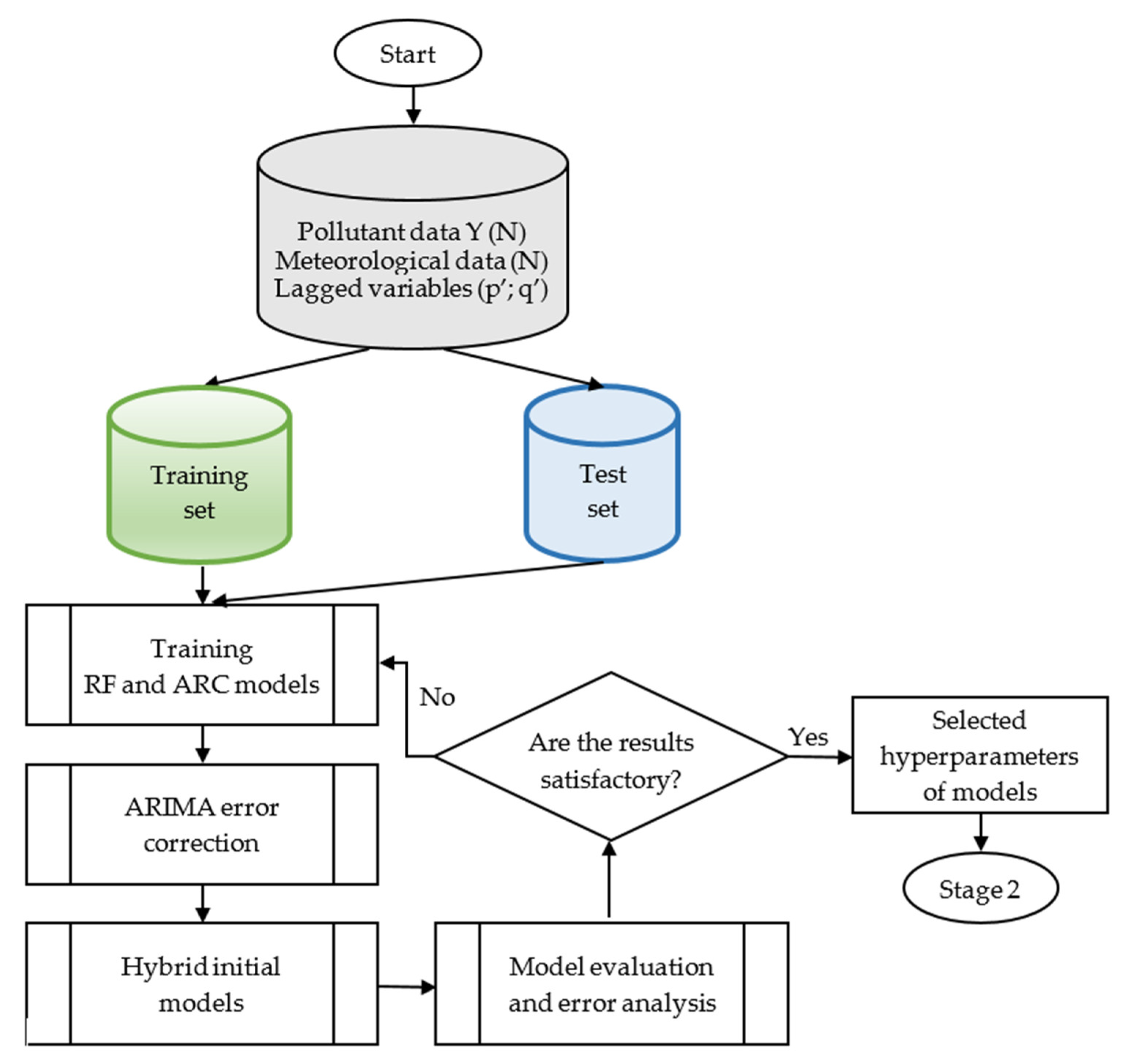
• Stage 1: Generating Initial Models

This is a procedure for building, calibrating, and selecting an initial model based on historical data of type (1) using a dataset of size $N=N_0$. For this purpose, we use known measured values for the dependent $\mathrm{Y}$ and independent variables $\mathrm{X}$. The first part of the data for $t=1,2,\hspace{0.17em}\mathrm{\dots }\hspace{0.17em},N_0-v$ will serve to train and validate the models, and the last $v$ values are for independent “out of sample” testing. This study uses $v=31$ or the test sample data for one month. The main result of this stage is the determination of optimal hyperparameters after evaluation of the data from testing and error correction using ARIMA. In this case, the models will become hybrids. A general scheme of the generation of the initial models in stage 1 is shown in Figure 1.

When this approach is applied over a long period of time, stage 1 may be periodically initialized to update the hyperparameters.

• Stage 2: Multi-Step Ahead Forecasting

This is the core of the proposed approach, which includes the following:

• Construction of single independent models and determining their predictions;
• Calculating averaged predictions (averaging models);
• Evaluation and comparison of the results.

The single independent models are built using the hyperparameters of the ML initial models, obtained in stage 1. The predictors are the measured data for air pollutants and independent time series, their values at previous moments (lagged variables), and forecasted (unmeasured) data for independent variables. For each given time period of horizons $s=1,2,\hspace{0.17em}\mathrm{\dots },\hspace{0.17em}S$, a separate single model is built and evaluated that predicts $h$ values as described in (4), (6). This is followed by a statistical evaluation of the models and residual diagnostics, including possible error correction with an appropriate ARIMA model.

The corresponding averaging models (5) are obtained by using the known forecasts of single models (6) in (7) up to a given horizon s (see also Table 1). The details of stage 2 are shown in Figure 2.

3.2. Model Assumptions

Each model is built on clearly defined assumptions that determine its limitations for practical application. It complies with

• using the ML regression-type method to construct forecasting models for multivariate time series dependent on predictors;
• predictor variables of qualitative and quantitative type;
• fixed forecasting horizon $h$.

In our implementation, only a limited number of factors affecting air pollutants are used, limited to those measured by state-certified automatic measuring stations in the Republic of Bulgaria, synchronized with European criteria [46]. In this study, time series of three pollutants and eight meteorological variables were used. In order to account for the influence of the remaining unmeasured factors, lagged variables containing deterministic and stochastic information on unmeasured factors were used. Predicted and unmeasured weather forecasts in the predictor variables are recorded by us day by day for the selected time period. However, such types of forecasts can be freely retrieved from multiple sources on the Internet for any major population location over 3-, 5-, and 10-day weather forecast time intervals.

As can be seen from (4), the approach enables the use of arbitrary predictors and is not limited to meteorological ones as in this study.

3.3. Methods

We will use two ensemble tree methods: RF and Arcing (variant arc-x4) (ARC). ARIMA will also be applied for residual correction to improve model accuracy and adequacy. Ensemble methods are presented and discussed, for example, in [47,48].

• Ensemble Model

An ensemble model is called the linear combination:

$$\overline{f}\left(x\right)={\displaystyle \sum _{j=1}^M{w}_j{f}_j\left(x\right)}.$$

(8)

with weights $w_j$ satisfying the conditions

$${\displaystyle \sum _{j=1}^M{w}_j=1,\hspace{0.17em}}\hspace{0.17em}\hspace{0.17em}\hspace{0.17em}\hspace{0.17em}\hspace{0.17em}\hspace{0.17em}0<w_j\le 1,\hspace{0.17em}\hspace{0.17em}j=1,2,\mathrm{\dots },M.$$

(9)

where $f_j\left(x\right),\hspace{0.17em}\hspace{0.17em}\hspace{0.17em}j=1,2,\mathrm{\dots },M$ are singular models created with the same algorithm for different perturbed samples $x$. In this paper, we will consider methods for which:

$$w_j=\frac{1}{M}.$$

(10)

In the case of regression, the final ensemble model is the arithmetic mean of the predictions of its constituent component models.

• Random Forest

The RF algorithm was developed by Leo Breiman in his well-known paper from 2001 [49], after combining his bagging idea with the random subspace method created by Tin Kam Ho in 1995 [50]. It can be briefly characterized as a bagged tree classifier using a majority vote. RF is a high-performance ensemble method with tens or hundreds of unpruned decision trees. Generally, RF applies to regression and classification for cross-sectional and time-series datasets with any type of variable. The same procedure is applied for the construction and training of each individual model (tree) $f_j\left(x\right)$ from the ensemble (8). Given an initial sample of size $n$, the RF algorithm selects a random sub-sample, called out-of-bag (OOB), comprising about one-third of all data to test the model. From the remaining up to $n$ instances onward, perturbed (randomized) samples are formed by subtraction with replacement using bagging [49]. A component tree is built using a recursive binary procedure with the formed sample. The resulting trees $f_j\left(x\right)$ are different and independent of each other. An important aspect of the RF algorithm is the random selection of a subset of all available predictors, called mtry (typically mtry = 3 to 5), when dividing the cases at each current node of the tree. The final RF model of mtree = $M$ is found by (8), (10). RF’s ability to calculate variable importance for each component tree and the composed ensemble model is useful for regression practice. It should be noted that RF is not particularly sensitive to the phenomenon of multicollinearity and is applicable even with highly correlated variables [51].

The main control hyperparameters set before the start of the RF algorithm are: mtree—the number of trees in an ensemble; nodesize—the size of the smallest allowable parent node; and mtry—the number of predictors randomly selected for splitting at each node. The last of these hyperparameters does not significantly affect the model’s results.

• Arcing

In this paper, we will apply the Arcing method (adaptively resample and combine), also known in the literature as Arc-x4. It was proposed and studied by Leo Breiman [52]. The algorithm is classified in the group of boosting methods, but it is relatively rarely used, and its predictive properties have not been sufficiently studied. This applies in particular to its ability to forecast time series. By the way, in [53], the authors show empirically that Arc-x4 outperforms all other algorithms from the boosting class for classification applied to real binary databases.

The algorithm induces an ensemble of sequentially dependent classifiers (models) $C_1,\hspace{0.17em}{C}_2,\hspace{0.17em}\mathrm{\dots }\hspace{0.17em},C_k,\hspace{0.17em}\mathrm{\dots },\hspace{0.17em}{C}_T$ for a number of trials $T$. At the k-th step, the classifier $C_k$ is training on the current resampled set $T_k$, and runs the original training set $T$ down $C_k$ by updating the probabilities $P^{(k+1)}$ for the next classifier $C_{k+1}$ by the expression

$$P^{(k+1)}(i)=\frac{1+m{(i)}^4}{{\displaystyle \sum \left(1+m{(i)}^4\right)}}.$$

(11)

where $m(i)$ is the total number of misclassifications of case $i$ by the previous classifiers $C_1,\hspace{0.17em}{C}_2,\hspace{0.17em}\mathrm{\dots }\hspace{0.17em},\hspace{0.17em}{C}_k.$ Unlike AdaBoost [54], classification is performed with unweighted voting, and in the case of regression, the prediction is averaged with equal weights according to (10). It is established that Arc-x4 reduced both the bias and variance of unstable models [52,53,55].

• Autoregressive Moving Average with Transfer Functions

The autoregressive moving average (ARIMA) is a linear type method, also known as the Box-Jenkins methodology [56], widely used for time series analysis and forecasting in statistics and econometrics. The main requirements for its application are the normality of data and stationarity, i.e., a constant mean and variance of the involved time series. However, in large sample sizes (e.g., where the number of observations per variable is greater than 10), violations of the normality assumption often do not noticeably impact the results [57]. In the more general case, the time series (1) may not be stationary and show a deterministic trend of some order (linear, quadratic, etc., up to some order $d).$ Let us denote the back-shift operator $B{Z}_t=Z_{t-1}$ with $\left(1-B\right)Z_t$. The transition to a stationary time series could be performed with a preliminary calculation of $d$ finite differences of the series with an operator of this type ${\left(1-B\right)}^d$. The one-dimensional (univariate) time series ARIMA (p, d, and q) model has the following form:

$$\left(1-{\displaystyle \sum _{j=1}^p{\varphi }_j{B}^j}\right){\left(1-B\right)}^d{Z}_t=\left(1-{\displaystyle \sum _{j=1}^q{\theta }_j{B}^j}\right)\hspace{0.17em}{a}_t+c,$$

(12)

where p, d, and q are model parameters, with constant non-negative integers for each $t$. Here, p is the number of autoregressive (AR) terms, $d$ is the order of differencing, q is the number of moving average (MA) terms $a_t$, and $c$ is an additive constant [56]. In Equation (12), ${\varphi }_1,{\varphi }_2,\mathrm{\dots },{\varphi }_p$ are estimates of the autoregressive part (AR) and ${\theta }_1,{\theta }_2,\mathrm{\dots },{\theta }_q$ are estimates of the moving average (MA).

When predictor time series (called transfer functions (TF)) are also used in the modeling, the method is called ARIMA/TF. Predictors are set with parameters (p, d, and q) of the same type. Model (12) takes the form:

$${\Delta }^d{Z}_t=\frac{MA}{AR}{a}_t+{\displaystyle \sum _{i=1}^k\left(\frac{Nu{m}_i}{De{n}_i}{\Delta }_i^{d_i}{B}^{b_i}{X}_{it}\right)+}\mu .$$

(13)

where $X_i,\hspace{0.17em}i=1,2,\hspace{0.17em}\mathrm{\dots }\hspace{0.17em},k$ are the predictor time series, ${\Delta }^d={\left(1-B\right)}^d,\hspace{0.17em}\hspace{0.17em}{\Delta }^{d_i}={\left(1-B\right)}^{d_i}$, $B^{b_i}$ is a delay term of positive integer order $b_i$, $MA,\hspace{0.17em}AR,\hspace{0.17em}Nu{m}_i,\hspace{0.17em}De{n}_i$ are difference polynomials, dependent on the predictor’s parameters, and $\mu$ is a constant [56].

• Hybrid method

Let us denote the generated and validated RF and ARC models at each prediction step s by Bs and their residuals by res_Bs with values

$$res\_B{s}_t=Y_t-B{s}_t.$$

(14)

If the corresponding ARIMA/TF model of res_Bs is Ar_res, built with the actual observations to forecast the entire considered period, then the hybrid model hBs and its residuals are calculated by

$$hBs=Bs+Ar\_res, res\_h=Y-h\_Bs.$$

(15)

3.4. Evaluation Measures

Let $Y$ be the observed true time series (target) and $P$ be the model prediction, $Y_i$ and $P_i$ $(i=1,2,\hspace{0.17em}\mathrm{\dots }\hspace{0.17em},n)$ are their values, respectively, $\overline{P},\hspace{0.17em}\hspace{0.17em}\overline{Y}$ are mean values, and $n$ is the sample size. The following well-known statistical measures of accuracy are considered to evaluate the prediction performance of the constructed ML models: Root mean squared error (RMSE), normalized relative mean squared error (NMSE), fractional bias (FB), Theil’s forecast accuracy coefficient $U_{II}$ [58], coefficient of determination ($R^2$), and index of agreement (IA) [59], given by the expressions:

$$RMSE=\hspace{0.17em}\sqrt{\frac{1}{n}{\displaystyle \sum _{i=1}^n{\left(Y_i-P_i\right)}^2}},\hspace{1em}\hspace{1em}\hspace{1em}NMSE=\hspace{0.17em}\frac{{\displaystyle \sum _{i=1}^n{\left(Y_i-P_i\right)}^2}}{{\displaystyle \sum _{i=1}^n{\left(Y_i-\overline{Y}\right)}^2}}$$

(16)

$$FB=\hspace{0.17em}2\frac{\overline{Y}-\overline{P}}{\overline{Y}+\overline{P}}\hspace{0.17em},\hspace{1em}\hspace{1em}\hspace{1em}{U}_{II}=\hspace{0.17em}\frac{\sqrt{{\displaystyle \sum _{i=1}^n{\left(Y_i-P_i\right)}^2}}}{\sqrt{{\displaystyle \sum _{i=1}^n{Y}_i^2}}}$$

(17)

$$R^2=\frac{{\left\{{\displaystyle \sum _{i=1}^n\left(P_i-\overline{P}\right)\left(Y_i-\overline{Y}\right)}\right\}}^2}{{\displaystyle \sum _{i=1}^n{\left(P_i-\overline{P}\right)}^2.}\hspace{0.17em}{\displaystyle \sum _{i=1}^n{\left(Y_i-\overline{Y}\right)}^2}},\hspace{1em}\hspace{1em}\hspace{1em}IA=1-\frac{{\displaystyle \sum _{i=1}^n{\left(P_i-Y_i\right)}^2}}{{\displaystyle \sum _{i=1}^n{\left(\left|P_i-\overline{Y}\right|+\left|Y_i-\overline{Y}\right|\right)}^2}}$$

(18)

RMSE and NMSE are used to assess the model’s accuracy. The FB index measures the tendency of a model to over-predict with values close to 2 and under-predict with values close to −2. IA is a dimensionless and bounded measure in $[0,\hspace{0.17em}1]$ with values closer to 1, indicating better agreement between the model and the target variable. The coefficient $U_{II}$ is dimensionless and is used to compare models obtained by different methods and to identify large values. The model is considered to be of good quality when $U_{II}$ is less than 1. A good predictive model should have a value close to 0 for RMSE, NMSE, and FB and a value close to 1 for $R^2$ and IA. It should be noted that using the RMSE and coefficient of determination $R^2$ to compare models and forecasts should be interpreted with care, as this may result in misleading conclusions ([60], Ch. 14). Also, statistical significance may be useful for small validation samples to judge whether accuracy differs among reasonable forecasting methods. For construct validity, the accuracy measures should agree ([60], Ch. 14).

Models and statistical analyses were performed using Salford Predictive Modeler 8.2 (SPM) [61] and IBM SPSS statistics software, version 28.0 [62,63] on a laptop (Acer, Intel Core i7, CPU 1.8 GHz).

3.5. Study Area and Data

The proposed approach from Section 3 was applied to predict the air pollutants in Pernik, a typical medium-sized city in Bulgaria. Pernik is located in western Bulgaria, about 20 km (12 miles) southwest of the capital Sofia, with a population of 70,000 as of 2021. The city is at an altitude between 700 and 850 m (2297 and 2789 feet), has a length of 22 km (14 miles), and is surrounded by three low mountains. Through the city flows the river Struma. The city’s territory is crossed by major roads, including Pan-European Corridors VIII and IV, which connect Central Europe and Greece. The climate of Pernik is moderately continental. Economically, the city is an industrial zone with steel production, heavy machinery (mining and industrial equipment), brown coal, building materials, and textiles. The location of Pernik is 42°36′ N 23°02′ E.

A dataset was collected for the concentration of three air pollutants (PM₁₀, SO₂, and NO₂) in the city of Pernik. Figure 3 shows the sequence plots of the pollutants. Daily data are modeled from 1 January 2015 to 9 February 2019. In the first stage, the training set is taken from 1 January 2015 to 21 December 2018 (1450 days), and the test period covers the next 31 days until 21 January 2019. The independent meteorological variables are eight: maximum air temperature (maxT, °C), minimum air temperature (minT, °C), wind speed (speed, m/s), wind direction (direction$), atmospheric pressure (press, mbar), cloud cover (cloud, %), relative humidity (humidity, %), and precipitation (precipi, mm). All measured data have been gathered from the official site of the automatic measuring station in Pernik [64,65] and the forecast weather data from the official site Sinoptik.bg.

4. Results

4.1. Preliminary Statistical Processing

The preliminary statistical processing of the data includes descriptive statistics, treatment of outliers and missing data, research on the multicollinearity of variables, and examination for sequence autocorrelation.

Descriptive statistics for the initial sample of n = 1481 cases are given in

Table 2. Summary statistics of the initial data for pollutants and meteorological variables.

	Variable	PM10 (μg/m3)	SO2 (μg/m3)	NO2 (μg/m3)	MaxT (°C)	MinT (°C)	Speed (m/s)	Humidity (%)	Pressure (mbar)	Cloud (%)	Precipi (mm)
Statistics
Valid		1411	1431	1434	1481	1481	1481	1481	1481	1481	1481
Missing		70	50	47	0	0	0	0	0	0	0
Mean		36.49	27.06	41.58	17.77	10.04	2.0004	0.694	1017.67	0.3197	1.759
Median		27.00	17.00	35.00	19.00	10.00	1.9400	0.700	1017.00	0.2500	0.000
Std. Deviation		30.309	45.114	28.920	10.527	10.243	0.8576	0.142	7.068	0.2629	4.0538
Variance		918.626	2035.244	836.351	110.815	104.914	0.736	0.020	49.957	0.069	16.433
Skewness		2.623	10.198	1.543	−0.151	−0.186	1.382	−0.088	0.248	0.707	4.284
Kurtosis		8.384	158.460	4.456	−0.925	−0.666	4.127	−0.747	0.463	−0.536	26.605
Minimum		2	1	0	−13	−27	0.28	0.31	990	0.00	0.0
Maximum		219	916	262	38	30	7.50	0.98	1039	1.00	44.0

. Of these, pollutant data for the last 31 days was used as an independent test sample in building the initial models. This part of the data can be seen in Figure 3 on the right side of the vertical blue lines on 22 December 2018. Missing data are below 5% for all samples. In the analyses, they are replaced by the method of linear interpolation. Also, Table 2 shows large values of the skewness and kurtosis for the three pollutants, speed and precipi. This is a sign that the distribution of these variables is not normal. This could affect the direct application of classical regression methods but not the ML techniques. In Table 2, large values are observed, particularly for PM₁₀ and SO₂. To reduce the influence of single spikes, available outliers of less than six cases are replaced by the values of their next largest value. We denote the obtained working variables for the pollutants as YPM10 (PM₁₀), YSO2 (SO₂), and YNO2 (NO₂). Their statistics are presented in the first three columns of Table 2. Figure 4 shows the boxplots of the distributions of these variables, used hereafter as dependents.

It is known that the accuracy of regression models could be affected by the presence of multicollinearity between variables. Statistical analysis was performed to check for bicorrelation in the data using the non-parametric Spearman’s Rho test. The Rho coefficients were the largest in absolute value only for (minT, maxT), equal to 0.969. All other Rho coefficients are less than 0.7. Since only 3 to 4 randomly selected predictors are used in the RF and ARC algorithms for each tree node splitting, we can assume that our data have no problematic multicollinearity.

Moreover, the autocorrelation functions (ACF) and partial ACF (PACF) plots of all considered time series showed that they do not exhibit trends. The ACF and PACF of YPM10 indicated large PACF coefficients for the first 2 to 3 lags, for YSO2 and YNO2—to the second lag, and for meteorological variables, an influence was found only for lag 1. Thus, in the general model (4), in our case, it is obtained $p^{\prime }\le 2,\hspace{0.17em}\hspace{0.17em}{q}^{\prime }\le 1$. That is, we will use lagged variables of the dependent variables up to the second order and for all predictors up to the first order.

In addition, in Figure 5 and

Table 3. Example data for measured values of wind direction and corresponding weather forecasts.

Day	Direction$	Direction$_f	Day	Direction$	Direction$_f
1	ESE	ESE	6	SW	SE
2	SE	SSE	7	S	SE
3	WSW	NNE	8	S	SSW
4	NE	NNE	9	ESE	W
5	NNW	N	10	SSW	S

, we give an example of a comparison of the measured values and forecasted weather conditions for one horizon of $h=10$ days used in this study. There are some pretty big inaccuracies in these weather forecasts, except for those about relative humidity.

4.2. Construction and Evaluation of the Initial Hybrid Models

A basic principle of forecasting is the construction of a model that well explains large historical variations in the dataset [60]. This is our first task. At this stage, the dependent variables YPM10, YSO2, and YNO2 of air pollutants PM₁₀, SO₂, and NO₂, respectively, and the eight meteorological variables are used. They cover a period of n = 1481 days from 1 January 2015 to 21 January 2019. Of these, the data for the first N1 = N-v = 1450 were used for training and validation, and the last v = 31 days were used as a hold-out (out-of-sample) test sample. Two lagged variables each were used for YPM10, YSO2, and YNO2, and one lagged variable each for all predictors was used for all initial ML models.

Multiple RF models were built and tuned varying for different selections of hyperparameters: number of trees in the model (mtree) from 100, 200, and 300; minimum number of cases for nodesize (5 and 10); and mtry = 3 and 4 for the random selection of predictors for splitting from a pool of 19 predictors. The models are trained with OOB procedures. Arcing models (denoted AR or ARC) were selected among models with 20, 30, 40, and 50 trees; a minimum number of cases in parents to child nodes was m1:m2 = 10:5, mtry = 3. ARC models were cross-validated (CV) with standard 5-fold and 10-fold CV. Here we follow the recommendation of [66] to use k-fold cross-validation over hold-out validation. Along with this, for greater precision, the initial models were also tested with a separate hold-out test sample of v = 31 days.

The hyperparameters for the RF models for the three pollutants showed close values: mtree = 300, nodesize = 5, and mtry = 3, OOB validation. The ARC models with the best statistics are ensembles with 50 trees, m1:m2 = 10:5, mtry = 3, 10-fold CV scheme.

From the built RF models, three models were selected, labeled TRF_P, TRF_S, and TRF_N, for PM₁₀, SO₂, and NO₂, respectively. Similarly, three ARC models were selected: TAR_P, TAR_S, and TAR_N. After a detailed examination of their residuals, it was found that there were weak autocorrelations. To ensure a lack of fit, ARIMA/TF models of the residuals were built for correction. All predictors were used as transfer functions. The corrections are added to the initial models to construct the hybrid test models using (14)–(15). They are denoted by hTRF_P, hTRF_S, etc. The basic descriptive statistics of the dependent variables YPM10, YSO2, and YNO2 were compared with these hybrid models in

Table 4. Descriptive statistics of the initial hybrid models for the test sample vs. measured values ^a.

Statistic	Pollutant Variables			Initial Hybrid Models
	YPM10	YSO2	YNO2	hTRF_P	hTAR_P	hTRF_S	hTAR_S	hTRF_N	hTAR_N
Mean	36.1249	25.4146	41.3707	36.046	36.306	25.377	25.730	41.283	42.244
Median	27.00	17.00	35.00	28.540	28.056	17.859	17.422	37.640	37.615
Std. Dev.	29.562	29.064	27.973	25.996	27.792	25.190	27.295	23.217	24.390
Variance	873.913	844.717	782.463	675.8	772.38	634.548	745.001	539.031	594.885
Skewness	2.551	2.932	1.281	2.412	2.632	2.355	2.892	1.058	1.241
Kurtosis	7.694	11.985	2.183	6.806	8.178	6.905	11.324	1.562	2.141
Minimum	2	1	0	6.311	8.295	0.379	0.457	0	0
Maximum	190	215	160	176.071	185.111	171.522	202.785	142.038	149.649

^a. the standard error of skewness for all variables is 0.064; the standard error of kurtosis for all variables is 0.127.

. Reasonably good agreement of the relevant descriptive statistics is observed for the RF and ARC models with YPM10, YSO2, and YNO2, respectively.

The following

Table 5. Performance statistics of the hybrid RF-ARIMA/TF and ARC_ARIMA/TF initial models.

Statistic	Initial Hybrid Models
	hTRF_P	hTAR_P	hTRF_S	hTAR_S	hTRF_N	hTAR_N
Variable	YPM10	YPM10	YSO2	YSO2	YNO2	YNO2
ARIMA/TF	(2,0,14)	(1,0,3)	(1,0,5)	(0,0,11)	(1,0,21)	(2,0,21)
Ljung-Box Sig.	0.231	0.454	0.905	0.304	0.360	0.154
RMSE	8.3182	6.0339	8.9356	7.2069	10.0499	8.9468
NMSE	0.0792	0.0417	0.0946	0.0615	0.1292	0.1024
FB	−0.0006	−0.005	0.001	−0.0123	0.0013	−0.0209
Uii	0.0046	0.0034	0.006	0.0049	0.0052	0.0047
IA	0.99998	0.99999	0.99998	0.99999	0.99997	0.99998
R2	0.932	0.960	0.932	0.966	0.884	0.905

presents the main performance results of the initial hybrid models. In row 4 the parameters of the ARIMA/TF models of the residuals are given. In their estimation, insignificant variables and lags were removed at the significance level $\alpha =0.05$ In row 5 are the estimated Ljung-Box test statistics for lack of fit applied to the residuals of the ARIMA/TF models [67]. All Ljung-Box statistics are insignificant at level $\alpha =0.05$, which allows to reject the null hypothesis, indicating that the models exhibit significant autocorrelations. For the six hybrid models in Table 5, the Ljung-Box test was applied to the 24 lags [68]. The last six rows of Table 5 present the statistics from (16)–(18). These show that all hybrid test models perform very well, with the ARC models outperforming the RF models with the exception of fractional bias.

Figure 6 illustrates the behavior of Ljung-Box coefficient significance values where the underlying process assumed independence (white noise).

Based on the performed diagnostics, we can conclude that the initial hybrid models are adequate and can be used to predict future pollutant values [33,68].

In particular, separately for all three dependent variables (YPM10, YSO2, and YNO2), the corresponding variable importance was established. In all three cases, the results indicated that the lagged variables of the targets, minimal air temperature, and wind speed are among the most important predictor variables for the training process.

4.3. Results from Stage 2—Multi-Step Forecasting

Following the algorithm in Figure 2, the built and calibrated initial models are extended step by step to calculate the h-day forecasts of the unknown concentrations of the three pollutants. All models use the already established hyperparameters from stage 1. A separate model is built according to (6) to predict each future horizon h.

For completeness, in Figure 7, we present the measured values of air pollutants for 17 days, which we further seek to predict. Some outliers are observed in the first seven days.

4.3.1. Construction and Evaluation of the Single Models

For each of the three pollutants, two single hybrid models were built-with RF and ARC. The models are labeled RF_P and AR_P (for PM₁₀), RF_S and AR_S (for SO₂), and RF_N and AR_N (for NO₂), respectively, at each horizon step $s,\hspace{0.17em}\hspace{0.17em}s=1,2,\hspace{0.17em}\mathrm{\dots },\hspace{0.17em}17$. The first prediction horizon (s = 1) starts from 15 January 2019 and uses data from 1 January 2015 to 14 January 2019 with known data plus 10 days ahead with forecasted meteorological data. This sets the value of the initial calibration data, where N₀ = 1474. The total number of single models needed to forecast 10 days ahead, performing s = 17 period steps, is 102.

From the obtained results, Figure 8 (in the left side Figure 8a,c,e,g,i) illustrate the evaluation statistics (16)–(18) of the horizon forecasts from all created single models. It is seen from Figure 8a that the RMSEs of model RF_P are smaller than those of model AR_P. The same ratios are observed for RF_N and AR_N. Similar are the results for RF_S and AR_S, at s > 6. The larger error values for s < 7 are probably due to the more difficult prediction of large outliers in the original data illustrated in Figure 7. In the case of NMSE in Figure 8c, we have similar results. Even here, the differences are larger in favor of RF models. In Figure 8f, the values of all FBs are in the interval (−0.65, 0.70) without large deviations and with a decreasing trend. The largest range is observed in FB for model AR_S. Figure 8g shows for Uii the same ratios as for NMSE. All of Theil’s Uii coefficients are less than 1. This indicates the models’ very good predictive performance (see also Section 3.4). The last figure in Figure 8i shows the IAs of the forecasts that vary strongly in the interval (0.1, 0.8). Here, the IA values of the RF models outperform, although less so than the corresponding values of the AR models. We have an exception for RF_N at s > 10. The overall conclusion is that, despite the better statistical performance of the initial AR models, the RF models do slightly better in predicting ex ante pollutant concentrations, and that is performed with highly changeable predictors.

4.3.2. Construction and Evaluation of the Averaging Models

After computing the 102 single models for each period step s, each with a horizon h, forecasts are obtained. They are averaged for each day by (7). The predictive averaging models are labeled aRF_P and aAR_P (for PM₁₀), aRF_S and aAR_S (for SO₂), and aRF_N and aAR_N (for NO₂). In our case, for horizon h = 10, we have calculated the forecast values for S = 17 periods.

From the obtained results, Figure 8b,d,f,h,j (right column) illustrate the corresponding evaluation accuracy statistics (16)–(18) for all created averaging models. Figure 8b shows RMSE behavior almost identical to that of single models. Especially for the last 10 horizons, in most cases, the RMSEs of the averaging models are smaller than the corresponding RMSEs of the single models. In particular, for PM₁₀ the aRF’s RMSE is equal to 13.1 μg/m³ vs. 13.8 μg/m³. For the NO₂ model, aRF shows 21.5 μg/m³ vs. 23.8 μg/m³. For SO₂, aAR has RMSE = 17.3 vs. 17.4, and for NO₂, the aAR model has RMSE = 22.7 vs. 27.5 for the single model, respectively. In Figure 8d, at s > 5 NMSEs, the averaging models appear more smoothed compared to the corresponding values of single models in Figure 8c. Here there is an exception for s = 17 in model AR_P. Fractional bias is within the same limits of [−0.65, 0.70] for all constructed models, as shown in Figure 8e,f. Also, all of Theil’s Uii coefficients are less than 1, which indicates a very good predictive ability for averaging models.

Although to a lesser extent, the other comparisons lead to the same general conclusion as for single models: a slightly pronounced superiority of RF models over AR. In the following two subsections, we will conduct statistical tests to check if there are statistically significant differences.

4.4. Comparison of the Accuracy Measures of the Forecasts

In this section, we compare the estimates of the statistical indicators (16)–(18) between the obtained final forecasts of the three pollutant targets (YPM10, YSO2, and YNO2) for the two methods and for the two multi-step-ahead prediction approaches. This does not include $R^2$ as noted in Section 3.4. For this purpose, we use Kendall tau-b rank correlation for paired samples, a nonparametric measure of the association between two sets of rankings. This statistic is useful for comparing methods when the number of forecasts is small, the distribution of the errors is unknown, or outliers (extreme errors) exist [60]. A higher positive correlation indicates better agreement between methods or models. The statistical significance of the coefficients is at level 0.05.

4.4.1. Comparison among the Two ML Methods

Table 6. Kendall’s correlations for comparison of the forecast accuracy, calculated using the two methods, RF and Arc-x4, for 17 period steps, each one for a prediction horizon of h = 10 steps ahead.

Statistic	RF_P, AR_P	RF_S, AR_S	RF_N, AR_N	aRF_P, aAR_P	aRF_S, aAR_S	aRF_N, aAR_N
RMSE	0.897	0.676	0.676	0.912	0.676	0.603
NMSE	0.838	0.382	0.397	0.926	0.368	0.412
FB	0.853	0.941	0.824	1.000	0.926	0.926
Uii	0.662	0.029 a	0.368	0.750	0.091 a	0.809
IA	0.618	0.471	0.574	0.706	0.647	0.029 a

^a Insignificant coefficients.

presents Kendall’s tau-b correlations of accuracy indicators for the pairs of models obtained with RF and Arcing methods. Good agreement among the methods for calculating accuracy measures (RMSE) with coefficients from 0.6 to 0.8 is observed. For NMSE, the correlations are high for PM₁₀ predictions (0.838 and 0.926); for the rest of the pairs, they are lower—around 0.4. The highest correlations are for FB for all model pairs (from 0.85 to 1.000). The correlations for AI are also high within the interval 0.5–0.7, except for the NO₂ models. For Uii, medium and high correlation values are obtained for the PM₁₀ and NO₂ models. The lower Uii correlations for some models of SO₂ (with low and insignificant correlations) can be explained by the few large outliers (see Figure 7). In general, following [60], it can be concluded that the correlations agree well, so the two methods exhibit almost equal predictive quality.

4.4.2. Comparison among the Two Multi-Step Ahead Strategies

In

Table 7. Kendall’s correlations for comparison of the forecast accuracy of single and averaging models for 17 period steps, each one for a prediction horizon of h = 10 steps ahead.

Statistic	RF_P, aRF_P	AR_P, aAR_P	RF_S, aRF_S	AR_S, aAR_S	RF_N, aRF_N	AR_N, aAR_N
RMSE	0.794	0.691	0.809	0.809	0.426	0.647
NMSE	0.824	0.794	0.647	0.779	0.309	0.618
FB	0.912	0.794	0.956	0.912	0.987	0.794
Uii	0.603	0.662	0.706	0.632	0.750	0.485
IA	0.338	0.544	0.294	0.088 a	0.632	0.324

^a. Insignificant coefficients.

, agreement among each pair of single and averaging models for five different statistical measures (16)–(18) of the forecasts (without R²) is presented. The correlations for RMSE are between 0.65 and 0.8, except for the NO₂ models. The NMSE coefficients are similar (from 0.6 to 0.83), and a lower coefficient is observed for the NO₂ models (0.309). The FB correlations show high values (0.8–0.99) for all model pairs. The correlations for Uii are medium to high, in the range of 0.49–0.75. The correlations for IA are weak, with an insignificant coefficient, except for 0.544 for (AR_P, aAR_P) and 0.632 for (RF_N, aRF_N). The results show reasonably good agreement among the forecasts of single and averaging models.

5. Discussion with Conclusions

In this study, we developed a multi-step ahead ex-ante forecasting strategy for time series with stochastic and high-frequency behavior. As shown in the preliminary study of the data (Table 2 and Figure 4 and Figure 5), the examined time series of air pollutants do not exhibit a normal distribution. They are characterized by many outliers that cannot be ignored. For the prediction of this type of data, we selected the ML methods RF and Arc-x4. We have previously explored many other methods to implement the modeling, including CART, MARS, LASSO, CART ensembles and bagging, stochastic gradient boosting, and more. We chose RF and ARC-x4 not only for their high statistical performance but also for their ability to predict new data well. The goal was to determine which ML methods are most suitable for achieving good results in a real-world situation. For the same reason, restrictions and assumptions are imposed on the predictors described in Section 3.2. Here, however, we must pay attention to the fact that lagged dependent variables were used as predictors, which indirectly reflected in a stochastic manner many other measurable and non-measurable factors influencing the pollution level. We have determined the approximate number of lags according to the behavior of the ACF and PACF of the dependent and meteorological variables. On this basis, a general form of the dependence in (4) is proposed. In this paper, we have chosen a short time horizon h of 10 days and repeated the experiments for 17 consecutive horizons (periods). We have yet to specifically investigate the most appropriate horizon length for the proposed strategy. This question remains open.

The developed forecasting strategy consists of two stages. The first stage is very important, with the selection and detailed examination of the candidate predictive models. First, RF and ARC models were created and analyzed, showing very good predictive properties, as can be seen from Table 5. The basic requirements for building models without autocorrelating residuals were carefully checked by examining the relevant ACF and using different statistical tests, including the Ljung-Box portfolio test. Some residuals were found to have values outside the confidence intervals. For this reason, all models had to be hybridized with the correction of their errors. This was done using the ARIMA method. Each hybrid model was calculated as a sum of the ML model and the ARIMA model of its residuals. The residuals of the hybrid methods were re-examined to obtain statistically valid models, checked by tests. Overall, the results on the right side of Table 5 suggest the hybrid initial ARC models outperform the RF models for all three pollutants.

The implementation of the second stage of the multi-step prediction required building a large number of single models for each horizon and each pollutant. The implementation turned out to be laborious. Updating the database should also be taken into account. For the first s = 1, 2,…, h periods, the forecasts are the average value of the available forecasts from the previous and current models. The final averaging models were found using (7). The application of the proposed approach was demonstrated for three different pollutants—PM₁₀, SO₂, and NO₂. The resulting final predictions were evaluated using five accuracy measures. The comparison of errors is illustrated in Figure 8 for both predictions of the single and averaging models. It is seen that the RF models achieve slightly more accurate predictions of tested future data in all cases. In addition, Kendall’s correlation was performed to compare the association between the accuracy of the two methods (RF and ARC) and the two strategies (single MIMO and averaging). In general, all indicators agree. Therefore, we can conclude that construct validity was obtained [60] and that both multi-step ahead approaches are alternatives.

Many studies have compared the performance of multi-step ahead strategies. However, due to the variety of modeling methods, accuracy criteria, and data, none of the existing strategies is known to be the best in all contexts. Nevertheless, the proposed approach can be formally compared with other results. For example, while in [37], the independent value prediction (Dir) was studied, in the present work, time series with predictors were used, ARIMA error correction was used, the data sets were updated dynamically, and more new elements were involved. The authors of the recent study [39] have employed all five strategies from Section 2 to forecast PM_2.5 for 10 days ahead. The best results among all constructed models were achieved using the recursive strategy with LASSO feature selection and forecasting the predictors in future time with the ARIMAX model. In one study, the direct strategy for hourly 1- to 24-step-ahead predictions of the air pollution index in Malaysia is preferred over other approaches [45]. A stacked ensemble with diverse ML modeling techniques using different strategies was adopted for PM_2.5 prediction in [39]. Existing multi-step ahead forecasting approaches have been thoroughly reviewed and compared empirically using 111 experimental datasets [38]. The authors concluded that multi-output strategies based on MIMO and DIRMO significantly outperform the single-output methods Rec, Dir, and DirRec. Our findings are primarily consistent with the results in [38].

Compared to the five standard multi-step ahead strategies, the proposed approach can be classified as an extension of the MIMO strategy and called MIMO averaging. It can also be noted that a large number of diverse ML methods are used in the subject area. To the best of our knowledge, the ability of Arc-x4 is examined for the first time in our study for multi-step ahead prediction. Although the limitations and assumptions of the models are laid out in this paper, the proposed MIMO averaging strategy is general. It can be applied to many different predictors, including dummy, land-use, or other types of variables. Some of the following questions remain open for further study: choice of horizon length; optimization of the coefficients in front of individual single models in the summation formula (7); the possibility of stacking the forecasts of single models built by diverse ML algorithms, and more.

For our data and the chosen horizon, h = 10, the proposed strategy is seen as an alternative to other multi-step ahead prediction methods. It can be used in comparison with or in conjunction with other approaches. Finally, we can conclude that the proposed MIMO averaging ex-ante forecasting strategy has the potential for real-world application and solving tasks of public interest, such as informing the population about the levels of the main air pollutants in a given local area.

References

1. World Health Organization, Regional Office for Europe. 2021. Review of Evidence on Health Aspects of Air Pollution—REVIHAAP Project: Technical Report. Available online: https://www.euro.who.int/__data/assets/pdf_file/0004/193108/REVIHAAP-Final-technical-report-final-version.pdf (accessed on 9 February 2023).
2. Gibson, J. Air pollution, climate change, and health. Lancet Oncol. 2015, 16, e269. [Google Scholar] [CrossRef] [PubMed]
3. Manisalidis, I.; Stavropoulou, E.; Stavropoulos, A.; Bezirtzoglou, E. Environmental and health impacts of air pollution: A review. Front. Public Health 2020, 8, 14. [Google Scholar] [CrossRef] [PubMed] [Green Version]
4. Rajagopalan, S.; Al-Kindi, S.; Brook, R. Air pollution and cardiovascular disease: JACC state-of-the-art review. J. Am. Coll. Cardiol. 2018, 72, 2054–2070. [Google Scholar] [CrossRef] [PubMed]
5. Tecer, L.; Alagha, O.; Karaca, F.; Tuncel, G.; Eldes, N. Particulate matter (PM 2.5, PM 10–2.5, and PM 10) and children’s hospital admissions for asthma and respiratory diseases: A bidirectional case-crossover study. J. Toxicol. Environ. Health A 2008, 71, 512–520. [Google Scholar] [CrossRef] [PubMed]
6. Sicard, P.; Augustaitis, A.; Belyazid, S.; Calfapietra, C.; de Marco, A.; Fenn, M.; Bytnerowicz, A.; Grulke, N.; He, S.; Matyssek, R.; et al. Global topics and novel approaches in the study of air pollution, climate change and forest ecosystems. Environ. Pollut. 2016, 213, 977–987. [Google Scholar] [CrossRef] [PubMed]
7. Ravindra, K.; Rattan, P.; Mor, S.; Aggarwal, A. Generalized additive models: Building evidence of air pollution, climate change and human health. Environ. Int. 2019, 132, 104987. [Google Scholar] [CrossRef]
8. Brasseur, G.P.; Jacob, D.J. Modeling of Atmospheric Chemistry; Cambridge University Press: Cambridge, UK, 2017. [Google Scholar]
9. Barratt, R. Atmospheric Dispersion Modelling: An Introduction to Practical Applications; Routledge: London, UK, 2013. [Google Scholar] [CrossRef]
10. Todorov, V.; Dimov, I.; Ostromsky, T.; Zlatev, Z.; Georgieva, R.; Poryazov, S. Optimized quasi-Monte Carlo methods based on Van der Corput sequence for sensitivity analysis in air pollution modelling. In Recent Advances in Computational Optimization. WCO 2020. Studies in Computational Intelligence; Springer: Cham, Switzerland, 2021; Volume 986, pp. 389–405. [Google Scholar] [CrossRef]
11. Ostromsky, T.; Dimov, I.; Georgieva, R.; Zlatev, Z. Air pollution modelling, sensitivity analysis and parallel implementation. Int. J. Environ. Pollut. 2011, 46, 83–96. [Google Scholar] [CrossRef]
12. Liu, Y.; Zhou, Y.; Lu, J. Exploring the relationship between air pollution and meteorological conditions in China under environmental governance. Sci. Rep. 2020, 10, 14518. [Google Scholar] [CrossRef]
13. Holst, J.; Mayer, H.; Holst, T. Effect of meteorological exchange conditions on PM10 concentration. Meteorol. Z. 2008, 17, 273–282. [Google Scholar] [CrossRef] [Green Version]
14. Veleva, E.; Zheleva, I. Statistical modeling of particle mater air pollutants in the city of Ruse, Bulgaria. MATEC Web Conf. 2018, 145, 01010. [Google Scholar] [CrossRef] [Green Version]
15. Tsvetanova, I.; Zheleva, I.; Filipova, M.; Stefanova, A. Statistical analysis of ambient air PM10 contamination during winter periods for Ruse region, Bulgaria. MATEC Web Conf. 2018, 145, 01007. [Google Scholar] [CrossRef] [Green Version]
16. Veleva, E.; Georgiev, R. Seasonality of the levels of particulate matter PM10 air pollutant in the city of Ruse, Bulgaria. AIP Conf. Proc. 2020, 2302, 030006. [Google Scholar] [CrossRef]
17. Tsvetanova, I.; Zheleva, I.; Filipova, M. Statistical study of the influence of the atmospheric characteristics upon the particulate matter (PM10) air pollutant in the city of Silistra, Bulgaria. AIP Conf. Proc. 2019, 2164, 120014. [Google Scholar] [CrossRef]
18. Siew, L.Y.; Chin, L.Y.; Wee, P.M.J. ARIMA and integrated ARFIMA models for forecasting air pollution index in Shah Alam, Selangor. Malays. J. Analyt. Sci. 2008, 12, 257–263. [Google Scholar]
19. Veleva, E.; Zheleva, I. GARCH models for particulate matter PM10 air pollutant in the city of Ruse, Bulgaria. AIP Conf. Proc. 2018, 2025, 040016. [Google Scholar] [CrossRef]
20. Lasheras, F.; Nieto, P.; Gonzalo, E.; Bonavera, L.; de Cos Juez, F. Evolution and forecasting of PM10 concentration at the Port of Gijon (Spain). Sci. Rep. 2020, 10, 11716. [Google Scholar] [CrossRef]
21. Feng, R.; Zheng, H.J.; Gao, H.; Zhang, A.R.; Huang, C.; Zhang, J.X.; Luo, K.; Fan, J.R. Recurrent Neural Network and random forest for analysis and accurate forecast of atmospheric pollutants: A case study in Hangzhou, China. J. Clean. Prod. 2019, 231, 1005–1015. [Google Scholar] [CrossRef]
22. Yazdi, D.; Kuang, Z.; Dimakopoulou, K.; Barratt, B.; Suel, E.; Amini, H.; Lyapustin, A.; Katsouyanni, K.; Schwartz, J. Predicting fine particulate matter (PM2. 5) in the greater London area: An ensemble approach using machine learning methods. Remote Sens. 2020, 12, 914. [Google Scholar] [CrossRef] [Green Version]
23. Masih, A. Application of ensemble learning techniques to model the atmospheric concentration of SO2. Glob. J. Environ. Sci. Manag. 2019, 5, 309–318. [Google Scholar] [CrossRef]
24. Bougoudis, I.; Iliadis, L.; Papaleonidas, A. Fuzzy inference ANN ensembles for air pollutants modeling in a major urban area: The case of Athens. In Proceedings of the International Conference on Engineering Applications of Neural Networks, Sofia, Bulgaria, 5–7 September 2004; Springer: Cham, Switzerland, 2014; pp. 1–14. [Google Scholar] [CrossRef]
25. Zhai, B.; Chen, J. Development of a stacked ensemble model for forecasting and analyzing daily average PM2.5 concentrations in Beijing, China. Sci. Total. Environ. 2018, 635, 644–658. [Google Scholar] [CrossRef]
26. Wang, P.; Liu, Y.; Qin, Z.; Zhang, G. A novel hybrid forecasting model for PM10 and SO2 daily concentrations. Sci. Total. Environ. 2015, 505, 1202–1212. [Google Scholar] [CrossRef] [PubMed]
27. Dairi, A.; Harrou, F.; Khadraoui, S.; Sun, Y. Integrated multiple directed attention-based deep learning for improved air pollution forecasting. IEEE Trans. Instrum. Meas. 2021, 70, 3520815. [Google Scholar] [CrossRef]
28. Sayegh, A.; Munir, S.; Habeebullah, T. Comparing the Performance of Statistical Models for Predicting PM10 Concentrations. Aerosol. Air Qual. Res. 2014, 14, 653–665. [Google Scholar] [CrossRef] [Green Version]
29. Sethi, J.K.; Mittal, M. A new feature selection method based on machine learning technique for air quality dataset. J. Stat. Manag. Syst. 2019, 22, 697–705. [Google Scholar] [CrossRef]
30. Xu, Y.; Liu, H.; Duan, Z. A novel hybrid model for multi-step daily AQI forecasting driven by air pollution big data. Air. Qual. Atmos. Health 2020, 13, 197–207. [Google Scholar] [CrossRef]
31. Pankratz, A. Forecasting with Dynamic Regression Models; John Wiley & Sons: New York, NY, USA, 1991. [Google Scholar]
32. Firmino, P.R.A.; de Mattos Neto, P.S.; Ferreira, T.A. Error modeling approach to improve time series forecasters. Neurocomputing 2015, 153, 242–254. [Google Scholar] [CrossRef]
33. Gocheva-Ilieva, S.; Voynikova, D.; Stoimenova, M.; Ivanov, A.; Iliev, I. Regression trees modeling of time series for air pollution analysis and forecasting. Neural Comput. Appl. 2019, 31, 9023–9039. [Google Scholar] [CrossRef]
34. Rybarczyk, Y.; Zalakeviciute, R. Machine learning approaches for outdoor air quality modelling: A systematic review. Appl. Sci. 2018, 8, 2570. [Google Scholar] [CrossRef] [Green Version]
35. Masih, A. Machine learning algorithms in air quality modeling. Glob. J. Environ. Sci. Manag. 2019, 5, 515–534. [Google Scholar] [CrossRef]
36. Ganchev, I.; Ji, Z.; O’Droma, M. A generic multi-service cloud-based IoT operational platform-EMULSION. In Proceedings of the 2019 International Conference on Control, Artificial Intelligence, Robotics & Optimization (ICCAIRO), Athens, Greece, 8–10 December 2019. [Google Scholar] [CrossRef]
37. Cheng, H.; Tan, P.-N.; Gao, J.; Scripps, J. Multistep-ahead time series prediction. Lect. Notes Comput. Sci. 2006, 3918, 765–774. [Google Scholar] [CrossRef]
38. Taieb, S.B.; Bontempi, G.; Atiya, A.F.; Sorjamaa, A. A review and comparison of strategies for multi-step ahead time series forecasting based on the NN5 forecasting competition. Expert Syst. Appl. 2012, 39, 7067–7083. [Google Scholar] [CrossRef] [Green Version]
39. Ahani, I.; Salari, M.; Shadman, A. Statistical models for multi-step-ahead forecasting of fine particulate matter in urban areas. Atmos. Pollut. Res. 2019, 10, 689–700. [Google Scholar] [CrossRef]
40. Ahani, I.K.; Salari, M.; Shadman, A. An ensemble multi-step-ahead forecasting system for fine particulate matter in urban areas. J. Clean. Prod. 2020, 263, 120983. [Google Scholar] [CrossRef]
41. Kang, I.-B. Multi-period forecasting using different models for different horizons: An application to U.S. economic time series data. Int. J. Forecast. 2003, 19, 387–400. [Google Scholar] [CrossRef]
42. Liu, H.; Duan, Z.; Chen, C. A hybrid framework for forecasting PM2.5 concentrations using multi-step deterministic and probabilistic strategy. Air. Qual. Atmos. Health 2019, 12, 785–795. [Google Scholar] [CrossRef]
43. Vassallo, D.; Krishnamurthy, R.; Sherman, T.; Fernando, H. Analysis of random forest modeling strategies for multi-step wind speed forecasting. Energies 2020, 13, 5488. [Google Scholar] [CrossRef]
44. Galicia, A.; Talavera-Llames, R.; Troncoso, A.; Koprinska, I.; Martínez-Álvarez, F. Multi-step forecasting for big data time series based on ensemble learning. Knowl.-Based Syst. 2019, 163, 830–841. [Google Scholar] [CrossRef]
45. Mustakim, R.; Mamat, M.; Yew, H.T. Towards on-site implementation of multi-step air pollutant index prediction in Malaysia industrial area: Comparing the NARX neural network and support vector regression. Atmosphere 2022, 13, 1787. [Google Scholar] [CrossRef]
46. Air Quality Standards, European Commission. Environment. Available online: https://www.eea.europa.eu/themes/air/air-quality-concentrations/air-quality-standards (accessed on 9 February 2023).
47. Ren, Y.; Zhang, L.; Suganthan, P.N. Ensemble classification and regression-recent developments, applications and future directions. IEEE Comput. Intell. Mag. 2016, 11, 41–53. [Google Scholar] [CrossRef]
48. Zhou, Z.H. Ensemble Methods: Foundations and Algorithms; CRC Press: Boca Raton, FL, USA, 2012. [Google Scholar]
49. Breiman, L. Random forests. Mach. Learn. 2001, 45, 5–32. [Google Scholar] [CrossRef] [Green Version]
50. Ho, T.K. Random decision forests. In Proceedings of the 3rd International Conference on Document Analysis and Recognition, Montreal, QC, Canada, 14–16 August 1995; pp. 278–282. [Google Scholar]
51. Strobl, C.; Boulesteix, A.L.; Kneib, T.; Augustin, T.; Zeileis, A. Conditional variable importance for random forests. BMC Bioinform. 2008, 9, 307. [Google Scholar] [CrossRef] [PubMed] [Green Version]
52. Breiman, L. Arcing classifiers. Ann. Stat. 1998, 26, 801–824. [Google Scholar]
53. Khanchel, R.; Limam, M. Empirical comparison of boosting algorithms. In Classification—The Ubiquitous Challenge. Studies in Classification, Data Analysis, and Knowledge Organization; Weihs, C., Gaul, W., Eds.; Springer: Berlin/Heidelberg, Germany, 2005; pp. 161–167. [Google Scholar] [CrossRef]
54. Freund, Y.; Schapire, R.E. A decision-theoretic generalization of on-line learning and an application to boosting. J. Comp. Syst. Sci. 1997, 55, 119–139. [Google Scholar] [CrossRef] [Green Version]
55. Bauer, E.; Kohavi, R. An empirical comparison of voting classification algorithms: Bagging, boosting, and variants. Mach. Learn. 1999, 36, 105–139. [Google Scholar] [CrossRef]
56. Box, G.E.; Jenkins, G.M.; Reinsel, G.C.; Ljung, G.M. Time Series Analysis: Forecasting and Control; John Wiley & Sons: Hoboken, NJ, USA, 2015. [Google Scholar]
57. Schmidt, A.F.; Finan, C. Linear regression and the normality assumption. J. Clinic. Epidem. 2018, 98, 146–151. [Google Scholar] [CrossRef] [Green Version]
58. Bliemel, F. Theil’s forecast accuracy coefficient: A clarification. J. Mark. Res. 1973, 10, 444–446. [Google Scholar] [CrossRef]
59. Willmott, C. On the validation of models. Phys. Geogr. 1981, 2, 184–194. [Google Scholar] [CrossRef]
60. Armstrong, J.S. Principles of Forecasting: A Handbook for Researchers and Practitioners; Kluwer Academic: Boston, MA, USA, 2001. [Google Scholar]
61. SPM—Salford Predictive Modeler. 2022. Available online: https://www.minitab.com/enus/products/spm/ (accessed on 9 February 2023).
62. IBM SPSS Statistics 29. 2022. Available online: https://www.ibm.com/products/spss-statistics (accessed on 9 February 2023).
63. Yordanova, L.; Kiryakova, G.; Veleva, P.; Angelova, N.; Yordanova, A. Criteria for selection of statistical data processing software. IOP Conf. Ser. Mater. Sci. Eng. 2021, 1031, 012067. [Google Scholar] [CrossRef]
64. RIOSV Pernik: Monthly Monitoring of Atmospheric Air: Monthly Report on the Quality of Atmospheric air of Pernik according to Data from Automatic Measuring Station “Pernik-Center”. Available online: http://pk.riosv-pernik.com/index.php?option=com_content&view=category&id=29:monitoring&Itemid=28&layout=default (accessed on 9 February 2023). (In Bulgarian).
65. Pernik Historical Weather. Available online: https://www.worldweatheronline.com/pernik-weather-history/pernik/bg.aspx (accessed on 9 February 2023).
66. Yadav, S.; Shukla, S. Analysis of k-fold cross-validation over hold-out validation on colossal datasets for quality classification. In Proceedings of the 2016 IEEE 6th International Conference on Advanced Computing (IACC), Bhimavaram, India, 27–28 February 2016; pp. 78–83. [Google Scholar] [CrossRef]
67. Ljung, G.; Box, G. On a measure of lack of fit in time series models. Biometrika 1978, 65, 297–303. [Google Scholar] [CrossRef]
68. Fischer, B.; Planas, C. Large scale fitting of regression models with ARIMA errors. J. Off. Stat. 2000, 16, 173–184. [Google Scholar]
Figure 1. Flowchart of the algorithm of stage 1: Generating initial hybrid models.
Mathematics 11 01566 g001
Figure 2. Flowchart of the algorithm of stage 2: Multi-step ahead forecasting.
Mathematics 11 01566 g002
Figure 3. Sequence plots of the examined pollutant data: (a) PM10, (b) SO2, (c) NO2. The horizontal red line in (a) indicates the European and national standard for the upper daily PM10 limit of 50 μg/m3. The blue vertical lines separate the training and test samples.
Mathematics 11 01566 g003aMathematics 11 01566 g003b
Figure 4. Box-plots of the used variables YPM10, YSO2, and YNO2 for PM10, SO2, and NO2, respectively.
Mathematics 11 01566 g004
Figure 5. Measured meteorological values and their ex-ante weather forecasts (_f) for a 10-day horizon used in the multi-step procedure (example dataset): (a) MaxT, (b) MinT, (c) speed, (d) cloud, (e) precipi, (f) pressure, and (g) humidity.
Mathematics 11 01566 g005
Figure 6. Significance values of Ljung-Box coefficients for residuals of the initial hybrid test models.
Mathematics 11 01566 g006
Figure 7. Measured values of the three air pollutants to be predicted.
Mathematics 11 01566 g007
Figure 8. Comparison of the prediction accuracy statistics of all single models RF_ and AR_ (on the left) and the corresponding averaging models aRF_ and aAR_ (on the right): (a,b) RMSE; (c,d) NMSE; (e,f) FB; (g,h) Uii; (i,j) IA.
Mathematics 11 01566 g008aMathematics 11 01566 g008b