1. Introduction
Micro/nano-electromechanical systems (MEMS/NEMS) are miniaturized devices that operate at the micro/nanoscale and have a wide range of applications in various fields, including healthcare [
1], electronics, the automotive industry, aerospace, and defense [
2]. Micro/nano-beams are an important component of these systems because they can be used to transfer forces, displacements, and other mechanical quantities between different parts of the device. Some specific examples of the use of micro/nano-beams in MEMS/NEMS include:
Bio-MEMS [
1]: These are devices that use micro/nano-scale technology to interact with biological systems, such as cells, tissues, and organs. Micro/nano-beams can be used in bio-MEMS to create mechanical forces that stimulate or sense biological responses or to perform other functions such as drug delivery or tissue engineering.
Atomic force microscopes [
3]: These are advanced imaging tools that use a micro/nano-scale cantilever beam to probe the surface of a sample at a very high resolution. The beam is used to sense the interaction forces between the sample and the tip of the beam, which can be used to create a detailed map of the sample’s surface.
Micro-switches [
2]: These are tiny switches that can be used to control the flow of electrical current in a circuit. Micro/nano-beams can be used in micro-switches to actuate the switch and change the state of the circuit.
Micro-actuators [
4]: These are devices that can generate mechanical forces or displacements in response to an electrical or other input. Micro/nano-beams can be used as actuators in MEMS/NEMS to create small, precise movements.
Micro-resonators [
5]: These are devices that can vibrate at a specific frequency, and are used in a variety of applications including sensors, oscillators, and filters. Micro/nano-beams can be used to create the resonant motion in micro-resonators.
Micro-sensors [
6]: These are devices that can detect and measure physical quantities such as temperature, pressure, humidity, or chemical concentrations. Micro/nano-beams can be used in micro-sensors to sense these quantities and convert them into an electrical signal.
In addition to these examples, micro/nano-beams are also used in printers to improve the speed and quality of printing and to lower production costs and increase the number of dots per inch (dpi) [
7]. Overall, micro/nano-beams are a versatile and essential component of many micro/nano-electromechanical systems, and they have the potential to revolutionize a wide range of fields and applications [
8].
The mechanical and physical behavior of micro/nano-beams has been extensively studied through both experimental observations and theoretical methods [
9,
10].
To date, several studies have investigated various theories for modeling nano- and microsystems. These theories include continuum mechanics, molecular dynamics, and quantum mechanics, among others. Each theory has its own advantages and disadvantages, and the choice of which theory to use depends on the specific system being studied and the level of accuracy required. For example, continuum mechanics is widely used for modeling large-scale systems, while molecular dynamics and quantum mechanics are used for modeling small-scale systems at the atomic and subatomic level. Additionally, some theories have been developed specifically for nano and micro-systems, such as the non-local strain gradient theory, which takes into account the size-dependent behavior of these systems. Overall, there is a wide range of theories available for modeling nano- and micro-systems, and the choice of which theory to use should be made based on the specific characteristics and requirements of the system being studied [
11].
Molecular dynamic (MD) simulation allows for the analysis of nano-structures at the atomic level [
12]. However, this method can be time-consuming and may not be practical for all situations. On the other hand, the classical continuum mechanics theory, which is based on the study of large-scale materials, may not be accurate for the analysis of micro/nano-structures due to the lack of an additional length scale parameter and the importance of intermolecular forces on small scales. In addition, there are uncertainties about obtaining elasticity constants, such as the modulus of elasticity, using the discrete space model of micro/nano-structures with a continuum [
13]. To address these issues, the non-classical continuum theory has become a popular choice for the analysis of micro/nano-structures. It offers the benefits of not requiring a long time for analysis and being more accurate than classical continuum theory [
14]. Non-classical continuum theory includes various approaches, such as fractional calculus, which have been shown to be effective in the analysis of micro/nano-scale systems. In general, the use of non-classical continuum theory has become more prevalent in the analysis of micro/nano-structures due to its accuracy and efficiency compared to other methods [
15].
One of the non-classical continuum theories developed for modeling size-dependent beams is the couple stress theory [
16,
17]. The strain gradient theory, which takes into account the strain energy being a function of the amount of strain and its first derivative [
18], has been introduced in [
19], and the modified strain gradient theory has been proposed in [
20]. Similarly, the non-local elasticity theory [
21] considers the stress at a point as a function of strains at all points in the continuum, but only characterizes the softening effect and does not consider stiffness enhancement. However, strain gradient and couple stress theories can be used to incorporate stiffness enhancement. Therefore, the non-local elasticity theory, strain gradient theory, and couple stress theory address different aspects of size-dependent material behavior. Consequently, the combination of the non-local elasticity theory [
15] and the strain gradient theory [
22], called the non-local strain gradient theory [
23], is essential for accurately modeling real size-dependent mechanical behavior.
The nonlinear control of MEMS/NEMS has been a subject of significant research in recent years due to the importance of these micro/nano-scale systems in a variety of applications. The small size and high sensitivity of these systems make them prone to nonlinear behavior, which can affect their performance and stability [
24,
25]. Therefore, developing effective control strategies for nonlinear MEMS/NEMS systems is essential for ensuring their reliable operation. One approach that has been widely used for nonlinear control of MEMS/NEMS is sliding mode control (SMC). SMC is a robust control method that can effectively handle uncertainties and perturbations in the system, making it well-suited for micro/nano-scale systems where these factors can have a significant impact on performance.
SMC works by driving the system to a sliding surface in the state space, where the control input is applied in such a way as to maintain the system on the surface [
26,
27,
28,
29]. This allows the system to track a desired reference signal while rejecting external disturbances and uncertainties. There have been many successful applications of SMC to the nonlinear control of MEMS/NEMS systems. For example, it has been used to control the vibration of micro-resonators, stabilize the nonlinear dynamics of micro/nano-beams, and improve the performance of micro/nano-actuators. In these applications, SMC has been shown to be an effective method for improving the accuracy and reliability of micro/nano-scale systems. In addition to these practical applications, there has also been significant research on the theoretical foundations of SMC for nonlinear MEMS/NEMS systems, including the development of new control laws and the study of stability and convergence properties. Overall, the use of SMC for nonlinear control of MEMS/NEMS has proven to be a valuable tool for improving the performance and reliability of these systems [
30,
31,
32,
33]. On the other hand, the existence of faults and failures in most of the practical systems is undeniable, and this makes considering their effects in the design of controller essential [
34,
35]. These issues demand more studies on the controller techniques for micro/nano-beams.
The precise control and stabilization of small-scale systems are essential for the development of advanced technologies such as nano-robotics and micro-electromechanical systems (MEMS). However, the inherent uncertainties and potential for faults in these systems pose significant challenges for control design. To address these challenges, the authors propose a novel fault-tolerant terminal sliding mode control technique. The proposed controller includes a finite time estimator, the stability of which and the convergence of the error dynamics are established using the Lyapunov theorem. The effectiveness of the proposed control scheme and the high accuracy of the estimation algorithm are demonstrated through the simulation results. This research is novel in its approach to addressing the specific challenges that arise in the control of micro/nano-systems, and it has the potential to greatly improve the precision and robustness of small-scale systems, ultimately leading to the development of advanced technologies such as nano-robotics and MEMS.
The paper is structured as follows:
Section 2 introduces the mathematical model of a simply supported Euler–Bernoulli nano-beam subjected to a centralized force in the middle of the beam.
Section 3 presents the design of the proposed controller. In
Section 4, numerical simulations are presented to demonstrate the effectiveness and performance of the proposed control architecture and estimation algorithm for stabilizing the nonlinear vibration of the nano-beam. Finally, the conclusions are presented in
Section 5.
2. System Model and Mathematical Formulation
The strain energy (U) of an isotropic linear elastic material can be described using the non-local strain gradient theory [
23]:
where
,
, and
indicate the classical stress, the higher-order stress, and the normal strain, respectively. In addition, the one-dimensional differential operator is represented by
in which is equal to
. In addition,
and
can be defined as
where
,
, and
stand for the length of the nano-beam, the principal attenuation kernel function combining constitutive equations of the non-local effects, an additional kernel function relating to the non-local effect, and the Young’s modulus, respectively. In addition, the effects of the non-local elastic stress field are expressed by
and
. The strain gradient length scale parameter is represented by
. The general non-local strain gradient constitutive equation is given by [
23]:
where
is the Laplacian operator. Let
[
23] and Equation (5) can be rewritten as
Supposing
results in non-local elasticity theory as [
21]:
In addition, considering
, the strain gradient theory is given by [
22]
The structure of a hinged–hinged nano-beams is illustrated in
Figure 1.
Considering
Figure 1, the displacement components of a straight Euler–Bernoulli nano-beam can be represented as:
The displacements in the
x,
y, and
z directions are represented by
, and
, respectively. When considering large deflection and small slope for a straight Euler–Bernoulli nano-beam, Von Karman’s nonlinear strain relationship can be expressed as follows:
in which
denotes the longitudinal strain. The first variation of strain energy is given by:
Equation (11) can be rewritten as follows:
where
is the cross-sectional area. Now, we define the following stress resultants as:
where
and
are the classical normal moment and force, respectively; in addition,
and
indicate the non-classical ones. Substituting Equations (10) and (13) into Equation (12) results in:
In addition, for the work that is carried out by the applied external forces, one has:
where
and
represent the distributed axial and transverse loads, respectively. Similarly, the first variation of kinetic energy is given by:
where
The general form of Hamilton’s principle, which is used to derive the equations of motion, is as follows:
By applying Hamilton’s principle (18) and separating the coefficients of
and
, the governing equation of the system can be reached as follows:
Moreover, the corresponding boundary conditions are:
Equation (6) can be modified to apply to a nano-beam using the non-local strain gradient theory as follows:
According to Equations (13) and (21), one has:
where
Now, based on Equation (19), we substitute
and
into Equation (22), which yields:
Substituting Equation (19) in Equation (24) yields:
If we assume that the rotational inertia of the beam is negligible, the governing equation of the system, which is a function of
and its derivatives, can be written as follows:
According to Equation (26), it can be concluded that
remains unchanged. By integrating both sides of equation (26), we obtain the following equation:
where
is a constant parameter. The boundary condition for the hinged–hinged beam is:
By using the strain gradient theory [
22], as described in Equation (28), applying the boundary conditions related to the second derivatives and integrating both sides of Equation (27) over the length of the beam (from x = 0 to x = L), we can derive the following equation:
Substituting Equation (31) into Equation (25) results in the governing equation for the nano-beam based on the nonlocal strain gradient theory, which is expressed as follows [
15]:
To express Equation (32) in dimensionless form, the following quantities are introduced:
where
. Therefore, the dimensionless governing equation is obtained as:
where
In this study, we use the Galerkin approach to transform the partial differential equation into a nonlinear ordinary differential equation. To do this, we decompose the temporal and spatial terms of
as follows [
36]:
where
represents the unknown temporal component that needs to be determined, while
represents the spatial component of the transverse deflection that satisfies the boundary conditions of the hinged-hinged nano-beam.
In addition, the concentrated force
is given by:
Substituting Equations (36) and (37) in Equation (34), multiplying both sides of Equation (34) by
, and by calculating the integral over the length of the beam, the ordinary differential equation (ODE) will be obtained as follows:
where the dot denotes the derivative with respect to time, and coefficients
and
are given by:
where
and
are the fourth and sixth derivatives of
with respect to time, respectively, and
is its first derivative with respect to
. The state-space equation of the system is:
3. Controller Design
3.1. Problem Formulation
The non-local strain gradient nano-beams’ general state space in the presence of disturbance is described using the following form:
where
and
stand for the states of the system. It is noteworthy that here we design the controller for general cases in which n could be any number, and for the nano-beam
.
and
are nonlinear functions that describe the system dynamics.
represents the external control input, and
represents the disturbance.
According to the definitions of faults and failures presented in many sources, including [
37,
38,
39], faults and/or failures are modelled as follows:
where
is the actual control input;
indicates the desired control input; and
denotes the uncertain constant fault input. Parameter
is considered to be the actuator control effectiveness. The time profile of a fault affecting the actuator is represented by time-varying function
which is given by:
In this equation,
represents the unknown fault evolution rate, and
is the time of occurrence of the fault. An incipient fault occurs when
is small, while an abrupt fault occurs when
is large. The state space equation of the system in the presence of actuator faults and/or failures is given by:
Assumption 1. Uncertainties and disturbances are bounded, meaning there is a constant such that the norm of is less than or equal to d0 ().
Assumption 1 states that uncertainties and disturbances in the system are bounded, meaning there is a maximum limit on the magnitude of these disturbances, represented by a constant . This assumption can be mechanically motivated by the fact that in physical systems, disturbances and uncertainties are often caused by external factors such as environmental conditions, which are limited in their magnitude. For example, wind gusts or vibrations from nearby sources will have a maximum limit in terms of the forces they exert on the system.
Assumption 2. Due to the physical limitations on the actuators, control actions are constrained, i.e., . In addition, the additive fault is bounded, i.e., ≤ .
Assumption 2 states that control actions are constrained due to the physical limitations of the actuators, meaning there is a maximum limit on the magnitude of the control inputs, represented by a constant . Additionally, the assumption states that any additive fault in the system, represented by is also bounded with a maximum limit of u_0. This assumption can be mechanically motivated by the fact that actuators, such as motors and servos, have physical limitations on the amount of torque or force they can produce. Additionally, any additive faults in the system, such as sensor or actuator failures, will also have a maximum limit in terms of the impact they have on the system.
3.2. Finite-Time Disturbance-Observer-Based
To demonstrate the finite-time convergence of the closed-loop system and the error of the disturbance observer, Lemma 1 was utilized.
Lemma 1 [40]. Let Lyapunov function which fulfils the following inequality: The system will reach its equilibrium point in a finite time, as indicated by the following convergence time:where and . In the design process for the finite time estimator, the following auxiliary variables are defined:
where z is calculated by the following formula:
where
and
and
are odd positive integers. In addition, parameters
, and
are positive and
. The disturbance estimation
is given by:
Considering Equations (46), (49) and (50) yields:
Considering Equations (49)–(51), the following is achieved:
Theorem 1. The disturbance estimator (49)–(51) ensures that the error of disturbance estimation converges to zero in finite time.
Proof. Consider a Lyapunov function of the form:
The time derivative of the Lyapunov function is given by:
□
Considering Lemma 1 and Equation (54), it can be confirmed that in the finite time, the auxiliary variable s and, as a result, the disturbance estimation error converge to zero.
Herein, to design the fault-tolerant terminal sliding mode controller, the following sliding surfaces are defined:
We use the following recursive procedure to design nth sliding surface:
The
jth-order time derivative of
is calculated as follows:
On the basis of Equations (56) and (57), the following equation is obtained:
In accordance with Equations (45), (55) and (58) we have:
Finally, the disturbance-observer-based fault-tolerant tracking control law is given by:
where user-defined parameters
and
should be positive.
Theorem 2. The proposed control law (60) ensures that the states of the system (43) will converge to the desired value in finite time, even in the presence of uncertainties, external disturbances, and faults in the control actuators.
Proof. Substituting Equation (61) into Equation (60) yields:
In accordance with Equation (52), we know that after finite time
; thus, we obtain:
Now, assume a Lyapunov function candidate as:
the time derivative of V is given by:
□
Based on Lemma 1 and Equation (64), the states of the closed-loop system will converge to the equilibrium point in finite time, which completes the proof.
The block diagram of the proposed control technique is shown by
Figure 2. Based on Equation (60), the disturbances, as well as faults and failures, were considered in the model, and it makes the designed controller an appropriate and robust choice for the control of nano-beams.
4. Numerical Simulations
In this section, the numerical simulation for the stabilization of the nano-beam is demonstrated using the proposed control scheme. For numerical simulation, the parameters of the nano-beam are
; consequently, the exact value of the parameters that appeared in (38) is obtained as
,
, and
[
15].
The paper discussed the impact of using nonlocal parameters in modeling a system. Despite this, there may still be uncertainties present that make it necessary to use a disturbance observer. To address this, the proposed controller is specifically designed to work in conjunction with a powerful disturbance observer and reject the effects of all uncertainties. This allows for more accurate modeling and control of the system, despite any remaining uncertainties. Therefore, to better investigate real conditions for the nano-systems, we consider the external disturbance as:
The physical mechanisms of unexpected disturbances and faults in a nano-beam are varied and multifaceted. Some of the key factors that can contribute to these disturbances include thermal expansion or contraction, external forces such as mechanical stress, material defects, control actuator failure, and manufacturing errors.
Thermal expansion or contraction can cause the nano-beam to bend or deform in unexpected ways, leading to unexpected disturbances or faults. Similarly, external forces such as mechanical stress can cause the nano-beam to bend or deform, leading to unexpected disturbances or faults. Material defects such as cracks, voids, or impurities can weaken the nano-beam and make it more susceptible to unexpected disturbances or faults.
Control actuator failure can also cause unexpected disturbances or faults in a nano-beam, as the actuators may not work as intended and thus not provide the expected control on the nano-beam. Manufacturing errors such as improper alignment or uneven distribution of materials can also cause unexpected disturbances or faults in a nano-beam.
It is important to note that these disturbances and faults can be caused by a combination of multiple factors, and not all disturbances or faults are predictable. Therefore, the present research investigates the utilization of the non-local strain gradient theory and a novel fault-tolerant terminal sliding mode control technique to effectively address these disturbances and faults in the stabilization and control of an uncertain Euler–Bernoulli nano-beam with fixed ends.
The user-defined parameter of the control scheme is considered to be:
The control gains in the proposed control technique are selected through a process of trial and error. This process involves adjusting the control gains and evaluating the system’s performance until the desired level of performance is achieved.
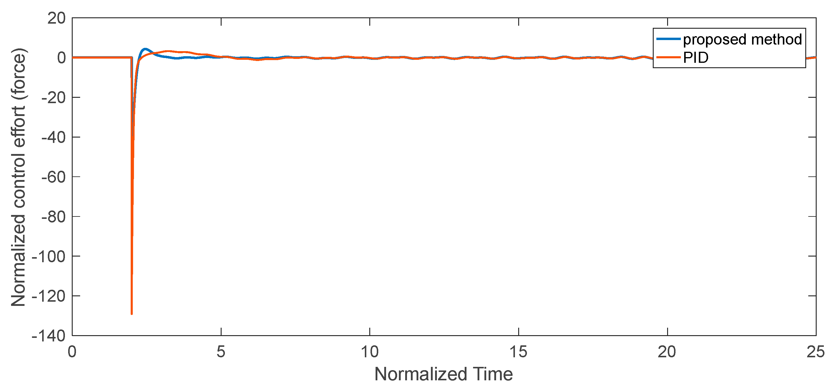
The performance of the proposed control technique has been compared with a PID controller in order to demonstrate its advantages. The control gain of PID is chosen as
,
, and
. In this case, we do not consider faults and failures in the actuators, and only the system is analyzed in the presence of external disturbances. The controller is turned on at
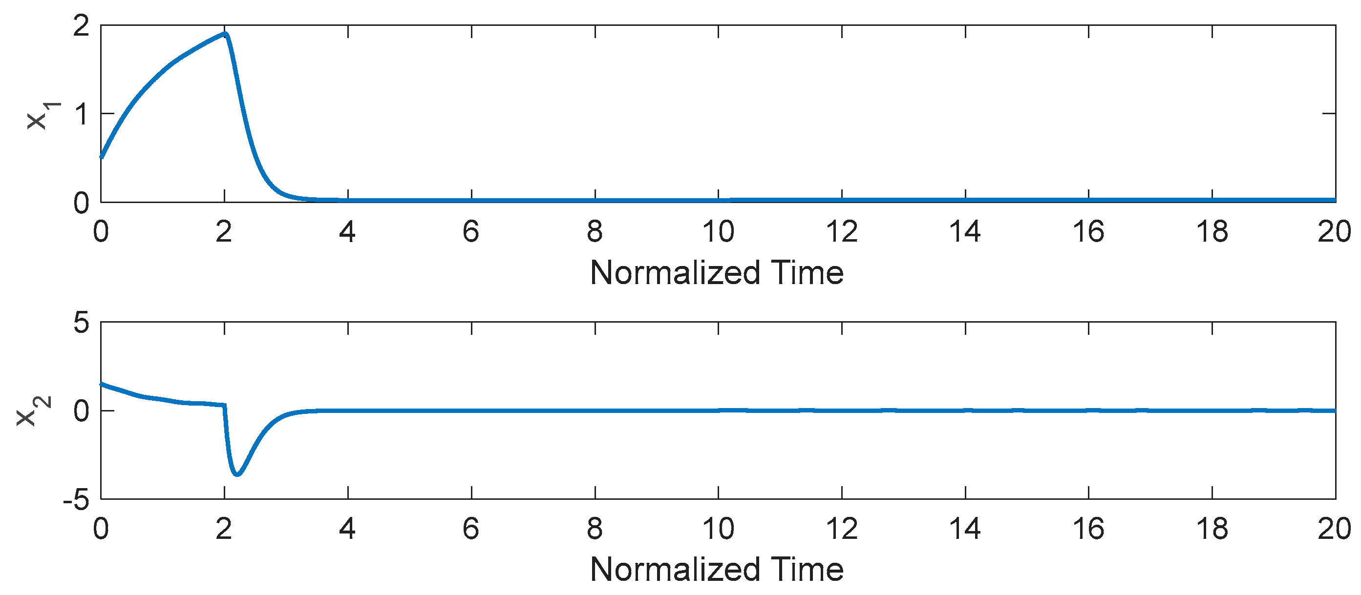
Figure 3 and
Figure 4 show the results of the stabilization of the nano-beam based on the proposed control technique and the PID controller. As can be seen in these figures, the proposed robust adaptive controller outperforms the PID controller. Additionally,
Figure 5 illustrates the excellent performance of the proposed disturbance observer, demonstrating its ability to effectively counteract disturbances and reject them entirely.
Now, we considered the nano-beam in the presence of faults and failure in the actuator. To this end, in addition to disturbances, the following faults and failure are considered for numerical simulations:
Figure 6,
Figure 7,
Figure 8 and
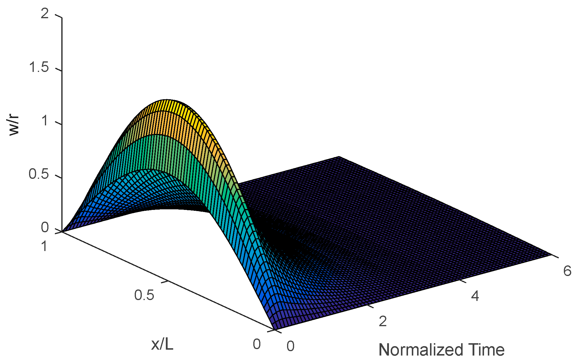
Figure 9 present the results of stabilizing the nano-beam using the proposed control technique in the presence of disturbances and faults. The controller is turned on at
.
Figure 6 demonstrates the time history of the deflection of nano-beam based on the proposed control scheme. Based on this figure, after one time unit, the nano-beam is completely stabilized.
Figure 7 demonstrates the time history of deflection of the nano-beam using the proposed control scheme. As is shown in these figures, the proposed controller, which is equipped with the fast estimator, could appropriately deal with uncertainties and faults in the actuator which is an important concern in the control nano-systems.
Figure 8 illustrates the performance of the controller in stabilizing the system. In addition, the performance of the estimator is depicted in
Figure 9. These results conspicuously confirm that by applying the suggested controller, the states of the system reach their desired values in a short period of time.
In summary, the numerical simulations vividly illustrate the effectiveness of the proposed control scheme for stabilization of the nano-beam when there exist unexpected disturbances and faults.

 ,
, 


