Some Latest Families of Exact Solutions to Date–Jimbo–Kashiwara–Miwa Equation and Its Stability Analysis

Abstract

The present study demonstrates the derivation of new analytical solutions for the Date–Jimbo–Kashiwara–Miwa equation utilizing two distinct methodologies, specifically the modified Kudryashov technique and the (g′)-expansion procedure. These innovative concepts employ symbolic computations to provide a dynamic and robust mathematical procedure for addressing a range of nonlinear wave situations. Additionally, a comprehensive stability analysis is performed, and the acquired results are visually represented through graphical representations. A comparison between the discovered solutions and those already found in the literature has also been performed. It is anticipated that the solutions will contribute to the existing literature related to mathematical physics and soliton theory.

1. Introduction

Many intricate natural phenomena have been described using nonlinear partial differential equations (NPDEs). Many researchers concentrate on this topic, since finding the exact solutions to these equations have enhanced our comprehension of how they function, how they are applied, and how they are created [1,2]. For the generalized Schrödinger equation, Hosseini et al. used a modified Jacobi elliptic expansion approach to discover exact solutions [3]. Fadhal et al. utilized exponential rational function (ERF) and modified simple equation (MSE) procedures to verify traveling wave solutions of the Sasa–Satsuma equation with beta derivative [4]. Zhang et al. obtained new solutions of the (2+1)-dimensional fractional KMM system consisting of Jacobi elliptic functions [5]. In the presence of cubic–quintic nonlinearity and fourth-order dispersion, Raza et al. were able to obtain novel optical solitons [6]. Ismael et al. worked on the modulation instability analysis of the coupled Schrödinger–Boussinesq system with the beta-derivative [7]. Zafar et al. handled some solutions to the DNA Peyrard–Bishop equation with the beta-derivative by use of the Kudryashov approach [8]. Martinez applied the subequation procedure [9]. Hosseini et al. obtained dark soliton solutions of some equations with the beta-derivative [10]. Pandir et al. employed the modified exponential function technique [11]. Yazgan et al. handled the sine-Gordon expansion method [12,13]. Ghanbari and Gomez Aguilar utilized the generalized exponential function procedure [14], Kudryashov employed the simplest equation method to the Chavy–Waddy–Kolokolnikov model [15], Sebogodi et al. applied the symmetry reduction method to (2+1)-dimensional combined potential Kadomtsev–Petviashvili-B-type Kadomtsev–Petviashvili [16], Sebogadi et al. used the ansatz method to obtain the traveling wave solutions of the generalized Chaffee–Infante equation in (1+3) dimensions [17], Podile et al. applied the multiple exp-function technique to the e (2+1)-dimensional Hirota–Satsuma–Ito equation [18], and so on [19,20,21,22,23].

We investigate the Date–Jimbo–Kashiwara–Miwa equation in this work with [24]:

$$u_{xxxxy}+4u_{xxy}{u}_x+2u_{xxx}{u}_y+6u_{xy}{u}_{xx}-2\upsilon u_{xxt}-\varrho u_{yyy}=0.$$

(1)

This equation is an integrable extension of the Kadomtsev–Petviashvili (KP) hierarchy [25]. The existence and uniqueness of the Kadomtsev–Petviashvili (KP) hierarchy solutions were proved in [26]. Numerical study of the Kadomtsev–Petviashvili (KP) equation were accurate, and the initial conditions are given in [27]. The efficient and well-established two-variable (G’/G, 1/G)-expansion procedure is employed to construct exact dynamical wave solutions for the Date–Jimbo–Kashiwara–Miwa equation. Through this approach, precise wave solutions are systematically generated with high efficiency and accuracy [28]. The (2+1)-dimensional Date–Jimbo–Kashiwara–Miwa equation has successfully shown N-soliton waves, fusion solutions, multiple M-lump solutions, and the collision phenomenon between one-M-lump and one or two soliton solutions [29]. Entirely novel complex analytical solutions for the governing model have been discovered for the Date–Jimbo–Kashiwara–Miwa equation, employing two potent approaches, namely SGEM and IBSEFM [30]. The multisoliton solutions for the Date–Jimbo–Kashiwara–Miwa equation are uncovered through the utilization of the Hirota simple technique, followed by the derivation of M-lump solutions for two types of time-dependent scenarios using the long-wave procedure [31]. Analytical soliton solutions for the (2+1)-dimensional Date–Jimbo–Kashiwara–Miwa equation are obtained by employing the extended tanh function procedure and the simple equation technique [32], Adem et al. derived the complexiton solutions with the help of the extended transformed rational function algorithm [33], Wazwaz furnished Painleve analysis to show that the equation is completely integrable in the Painleve sense [34].

The current work is arranged as follows: In Section 2, the main steps of the modified Kudryashov technique and $\left(g^{\prime }\right)$- expansion method are provided. In Section 3, we present the construction of precise solutions for the Date–Jimbo–Kashiwara–Miwa equation. Also, a graphical representation by taking parameters as special values and a stability analysis of the obtained solutions are given in Section 4. We present the discussion in Section 5. Some conclusions are shown in Section 6.

2. Techniques

In the current section, we present the modified Kudryashov technique and $\left(g^{\prime }\right)$-expansion algorithms. To this end, we first discuss the necessary auxiliary information as follows.

2.1. Auxiliary Information

For the purpose at hand, we postulate a system of NPDEs with the subsequent configuration:

$$P(u,u_t,u_x,u_y,u_{tt},u_{xt},u_{xx},\dots )=0,$$

(2)

wherein P incorporates u and its diverse partial derivatives with respect to t and classical derivatives with respect to x and $y.$

The wave transformation can be expressed in the following manner:

$$u(x,y,t)=u\left(\xi \right),\xi =kx+\gamma y-\omega t,$$

(3)

where $k,\gamma$, and $\omega$ are constants to be determined. Subsequently, Equation (3) is substituted into Equation (2), leading to the discovery of a system of equations. This system is then solved to establish the conditions for the parameters and utilize the obtained results. Consequently, we obtain the following ordinary differential equation (ODE), which will be integrated the possible amount of times with respect to $\xi .$

$$Q(u,u^{\prime },u^{\prime \prime },\dots )=0$$

(4)

2.2. The Modified Kudryashov (MK) Technique

In accordance with the methodology, the solutions to Equation (4) are represented in the following manner [35,36,37,38]:

$$u\left(\xi \right)=\stackrel{N}{\sum _{i=0}}{\varpi }_i{\left(\psi \left(\xi \right)\right)}^i,{\varpi }_N\ne 0,$$

(5)

where ${\varpi }_i\left(i=0,1,\dots ,N\right)$are constants that are determined later, N is calculated by the homogeneous balance principle, and the function $\psi \left(\xi \right)$ is given by:

$$\psi \left(\xi \right)=\frac{1}{1+\chi a^{\xi }},$$

(6)

where Equation (6) satisfies the following ODE:

$${\psi }^{\prime }\left(\xi \right)=\left({\psi }^2\left(\xi \right)-\psi \left(\xi \right)\right)lna.$$

(7)

By surrogating the Equation (5) into Equation (4) while taking into account Equation (7), a system of algebraic equations is derived involving ${\varpi }_m,a,k,\gamma ,\chi$, and $\omega .$Ultimately, by solving this system of equations, the exact solutions for Equation (2) can be computed.

2.3. The (g′)-Expansion Procedure

We hypothesize that the solution to Equation (4) can be expressed in the following manner:

$$u\left(\xi \right)=\sum _{i=0}^N{a}_i{\left(g^{\prime }\right)}^i.$$

(8)

Here, the constants $a_i(i=0,\dots ,N)$ are yet to be determined and are found at a later stage. The value of N is determined using the procedure of homogeneous balance. Here, the function g fulfills the following ODE:

$$g^{\prime \prime }=a+b{g}^{\prime }+c{g^{\prime }}^2.$$

(9)

The solutions of Equation (9) can be expressed as follows:

1: When the discriminant $\Delta =4ac-b^2$ is less than zero, the solution is defined as follows:

$$g=\frac{1}{2c}\left[ln\left({tanh}^2\left(\frac{\xi \sqrt{-\Delta }}{2}\right)-1\right)-b\xi \right],$$

and

$$g^{\prime }=\frac{1}{2c}\left[\sqrt{-\Delta }tanh\left(-\frac{\xi \sqrt{-\Delta }}{2}\right)-b\right].$$

(10)

2: When the discriminant $\Delta =4ac-b^2$ is equal to zero, the solution is defined as follows:

$$g=-\frac{1}{c}\left[ln\left(\xi \right)+\frac{\xi b}{2}\right],$$

and

$$g^{\prime }=-\frac{1}{c}\left(\frac{1}{\xi }+\frac{b}{2}\right).$$

(11)

3: When the discriminant $\Delta =4ac-b^2$ is greater than zero, the solution is defined as follows:

$$g=\frac{1}{2c}\left[ln\left({tan}^2\left(\frac{\xi \sqrt{\Delta }}{2}\right)+1\right)-b\xi \right],$$

and

$$g^{\prime }=\frac{1}{2c}\left[\sqrt{\Delta }tan\left(\frac{\xi \sqrt{\Delta }}{2}\right)-b\right].$$

(12)

By substituting Equation (8) into Equation (4) along with Equation (9) and the coefficients of all powers of ${\left(g^{\prime }\right)}^i$ to zero, we attain a system of equations. This obtained system encompasses the variables $a_i(i=0,\dots ,N),a,b,c,k,\gamma$, and $\omega$. Solving these determining equations enables us to obtain the values of $a_i$ and $\omega .$ Substituting these derived values into (8), along with Equations (10)–(12), yields all feasible solutions [39,40,41].

3. Application of the Methods

In this particular section of the study, our objective is to seek new traveling wave solutions for Equation (1). To accomplish this, we commence by conducting a mathematical analysis of the problem at hand.

3.1. Mathematical Analysis

If we substitute Equation (3) into Equation (1), the following equation can be derived:

$$k^4\gamma u^{\left(5\right)}+6k^3\gamma {\left(u^{\prime \prime }{u}^{\prime }\right)}^{\prime }-(\varrho {\gamma }^3-2k^2\upsilon \omega )u^{\prime \prime \prime }=0.$$

(13)

Integrating Equation (13) with respect to $\xi$ twice and assuming the integral constants are zero, we find

$$k^4\gamma u^{\prime \prime \prime }+3k^3\gamma {\left(u^{\prime }\right)}^2-(\varrho {\gamma }^3-2k^2\upsilon \omega )u^{\prime }=0$$

(14)

setting $u^{\prime }=U$ in Equation (14), we acquire the ensuing equation:

$$k^4\gamma U^{\prime \prime }+3k^3\gamma U^2-(\varrho {\gamma }^3-2k^2\upsilon \omega )U=0$$

(15)

We obtain the balancing number as $N=2$ if we balance $U^2$ with $U^{\prime \prime }.$

3.2. Application of the MK Procedure

In this subsection, we demonstrate the utilization of the MK procedure. If we take an auxiliary solution for Equation (15) as follows:

$$U\left(\xi \right)={\varpi }_0+{\varpi }_1\psi \left(\xi \right)+{\varpi }_2{\left(\psi \left(\xi \right)\right)}^2,$$

(16)

then substitute the Equation (16) in Equation (15) without ignoring Equation (7), and then collect the coefficients of the ${\psi }^i\left(\xi \right),$ we obtain the determining equation system as follows:

$$\begin{array}{ccc}\hfill & \hfill & 6\gamma ln{\left(a\right)}^2{\varpi }_2{k}^4+3\gamma {\varpi }_2^2{k}^3=0,\hfill \\ \hfill & \hfill & 2\gamma ln{\left(a\right)}^2{\varpi }_1{k}^4-10\gamma ln{\left(a\right)}^2{\varpi }_2{k}^4+6\gamma {\varpi }_1{\varpi }_2{k}^3=0,\hfill \\ \hfill & \hfill & 3\gamma ln{\left(a\right)}^2{\varpi }_1{k}^4+4\gamma ln{\left(a\right)}^2{\varpi }_2{k}^4+6\gamma {\varpi }_0{\varpi }_2{k}^3+3\gamma {\varpi }_1^2{k}^3-{\gamma }^3{\varpi }_2\varrho +2{\varpi }_2{k}^2\upsilon \omega =0,\hfill \\ \hfill & \hfill & \gamma ln{\left(a\right)}^2{\varpi }_1{k}^4+6\gamma {\varpi }_0{\varpi }_1{k}^3-{\gamma }^3{\varpi }_1\varrho +2{\varpi }_1{k}^2\upsilon \omega =0,\hfill \\ \hfill & \hfill & 3\gamma k^3{\varpi }_0^2+2k^2{\varpi }_0\upsilon \omega -\varrho {\gamma }^3{\varpi }_0=0.\hfill \end{array}$$

If we solve the obtained system, we obtain solution families as follows:

Case 1:

$$\left\{{\varpi }_0\to 0,{\varpi }_1\to 2ln{\left(a\right)}^{2}k,{\varpi }_2\to -2ln{\left(a\right)}^{2}k,\omega \to \frac{\gamma \left(-ln{\left(a\right)}^2{k}^4+{\gamma }^2\varrho \right)}{2k^2\upsilon }\right\}$$

(17)

If we substitute the obtained values of the coefficients (17) in Equation (16) without ignoring Equation (6) and relation $u^{\prime }=U$, we obtain the following solution:

$$u\left(x,y,t\right)=-\frac{2ln\left(a\right)k}{1+\chi a^{kx+\gamma y-\omega t}}$$

(18)

Case 2:

$$\left\{{\varpi }_0\to -\frac{ln{\left(a\right)}^{2}k}{3},{\varpi }_1\to 2ln{\left(a\right)}^{2}k,{\varpi }_2\to -2ln{\left(a\right)}^{2}k,\omega \to \frac{\gamma \left(ln{\left(a\right)}^2{k}^4+{\gamma }^2\varrho \right)}{2k^2\upsilon }\right\}$$

(19)

If we use values (19) with the same procedure above, we obtain the following exact solution:

$$u\left(x,y,t\right)=-\frac{ln{\left(a\right)}^{2}k\left(kx+\gamma y-\omega t\right)}{3}-\frac{2ln\left(a\right)k}{1+\chi a^{kx+\gamma y-\omega t}}$$

(20)

3.3. Application of the $\left(g^{\prime }\right)$-Expansion Procedure

We organize this subsection to demonstrate the application of the $\left(g^{\prime }\right)$-expansion technique to the given equation. If we take an auxiliary solution for Equation (15) as follows:

$$U\left(\xi \right)=a_0+a_1\psi \left(\xi \right)+a_2{\left(\psi \left(\xi \right)\right)}^2,$$

(21)

then substitute the Equation (21) in Equation (15) without ignoring Equation (9), and then collect the coefficients of the ${\left(g^{\prime }\right)}^i,$ we obtain the determining equation system as follows:

$$\begin{array}{ccc}\hfill & \hfill & 6a_2{k}^4{c}^2\gamma +3a_2^2{k}^3\gamma =0,\hfill \\ \hfill & \hfill & 2a_1{k}^4{c}^2\gamma +10a_{2}b{k}^{4}c\gamma +6a_1{a}_2{k}^3\gamma =0,\hfill \\ \hfill & \hfill & 8a{a}_2{k}^{4}c\gamma +3a_{1}b{k}^{4}c\gamma +4a_2{b}^2{k}^4\gamma +6a_0{a}_2{k}^3\gamma +3a_1^2{k}^3\gamma +2a_2{k}^2\upsilon \omega -a_2{\gamma }^3\varrho =0,\hfill \\ \hfill & \hfill & 2a{a}_1{k}^{4}c\gamma +6a{a}_{2}b{k}^4\gamma +a_1{b}^2{k}^4\gamma +6a_0{a}_1{k}^3\gamma +2a_1{k}^2\upsilon \omega -a_1{\gamma }^3\varrho =0,\hfill \\ \hfill & \hfill & 2\gamma k^4{a}_2{a}^2+\gamma k^4{a}_{1}ba+3\gamma k^3{a}_0^2+2k^2\upsilon \omega a_0-\varrho {\gamma }^3{a}_0=0.\hfill \end{array}$$

If we solve the obtained system, we obtain solution families as follows:

Case 1:

$$\left\{a_0\to -2ack,a_1\to -2bck,a_2\to -2k{c}^2,\omega \to \frac{\gamma \left(4ac{k}^4-b^2{k}^4+{\gamma }^2\varrho \right)}{2k^2\upsilon }\right\}$$

(22)

(i)

If $4ac-b^2<0$, the solution is given by

$$u\left(x,y,t\right)=-\frac{k\left(4ac-b^2\right)tanh\left(\frac{\left({}^{kx+\gamma y-\omega t}\right)\sqrt{-4ac+b^2}}{2}\right)}{\sqrt{-4ac+b^2}}.$$

(23)

(ii)

If $4ac-b^2=0,$ the solution is given by

$$u\left(x,y,t\right)=-\frac{k\left(\left(4ac-b^2\right)\left({}^{kx+\gamma y-\omega t}\right)-\frac{4}{\left({}^{kx+\gamma y-\omega t}\right)}\right)}{2}.$$

(24)

(iii)

If $4ac-b^2>0,$ the solution is given by

$$u\left(x,y,t\right)=-k\sqrt{4ac-b^2}tan\left(\frac{\left({}^{kx+\gamma y-\omega t}\right)\sqrt{4ac-b^2}}{2}\right).$$

(25)

Case 2:

$$\left\{a_0\to -\frac{2}{3}ack-\frac{1}{3}{b}^{2}k,a_1\to -2bck,a_2\to -2k{c}^2,\omega \to \frac{\gamma \left(-4ac{k}^4+b^2{k}^4+{\gamma }^2\varrho \right)}{2k^2\upsilon }\right\}$$

(26)

(i)

If $4ac-b^2<0$, the solution is given by

$$u\left(x,y,t\right)=-\frac{k\left(4ac-b^2\right)\left(\left({}^{kx+\gamma y-\omega t}\right)\sqrt{-4ac+b^2}-3tanh\left(\frac{\left({}^{kx+\gamma y-\omega t}\right)\sqrt{-4ac+b^2}}{2}\right)\right)}{3\sqrt{-4ac+b^2}}.$$

(27)

(ii)

If $4ac-b^2=0,$ the solution is given by

$$u\left(x,y,t\right)=-\frac{k\left(\left(4ac-b^2\right)\left({}^{kx+\gamma y-\omega t}\right)-\frac{12}{\left({}^{kx+\gamma y-\omega t}\right)}\right)}{6}.$$

(28)

(iii)

If $4ac-b^2>0,$ the solution is given by

$$u\left(x,y,t\right)=\frac{k\sqrt{4ac-b^2}\left(\left({}^{kx+\gamma y-\omega t}\right)\sqrt{4ac-b^2}-3tan\left(\frac{\left({}^{kx+\gamma y-\omega t}\right)\sqrt{4ac-b^2}}{2}\right)\right)}{3}.$$

(29)

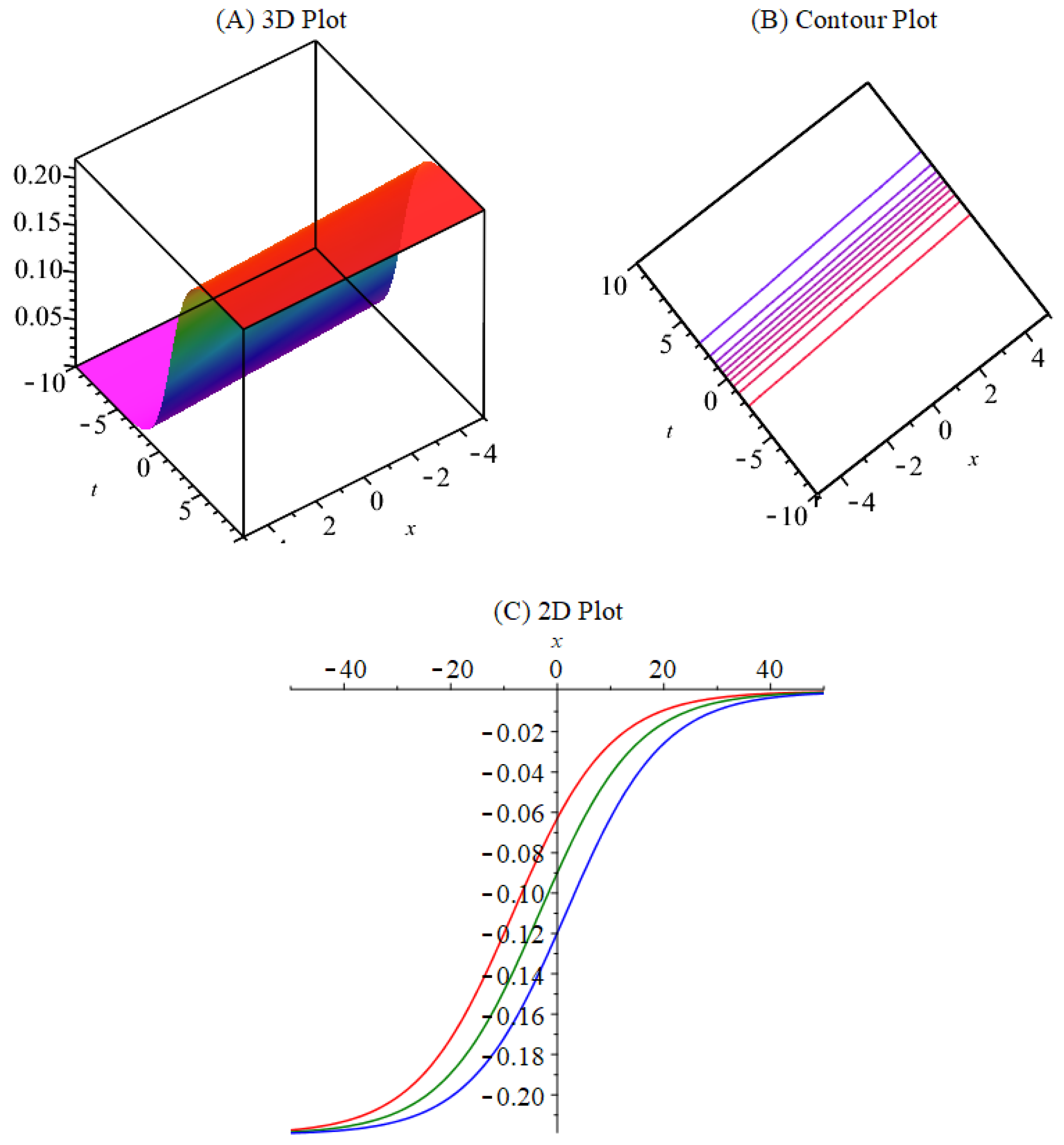
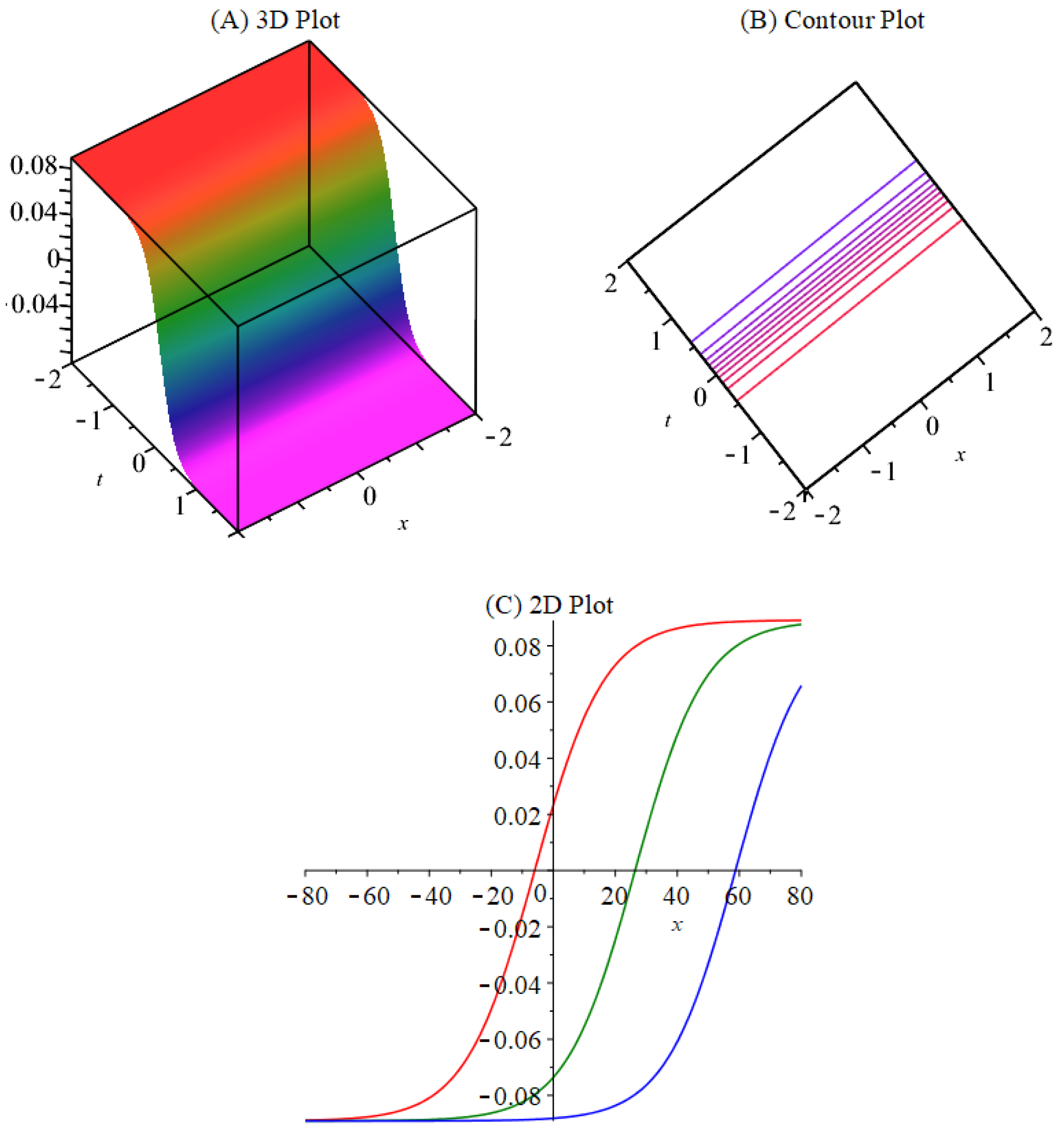
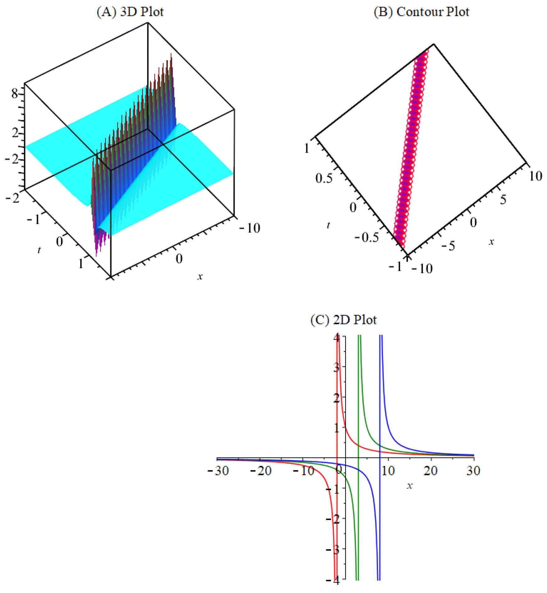
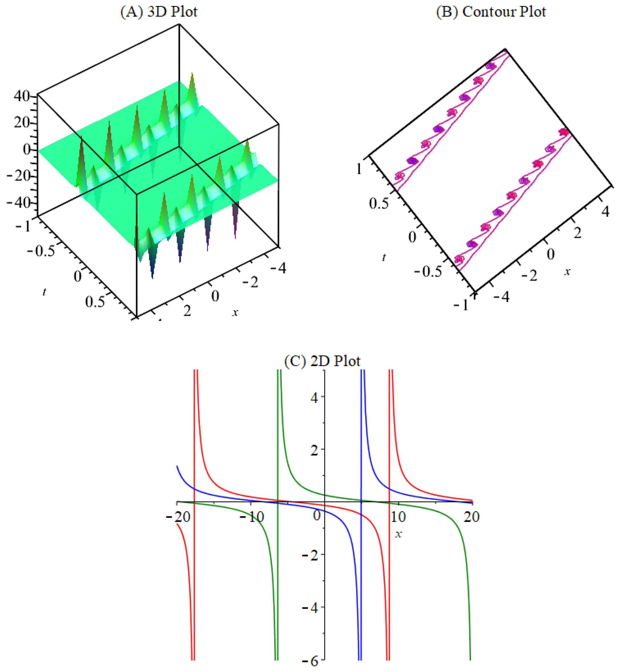
4. Stability Analysis and Figures

The stability property of the solutions are closely related to the momentum in the Hamilton system. Kao and Pasumarthy studied the relation of the stability analysis and Hamiltonian systems in [42]. From this point of view, the following formula is given for the Hamiltonian system of the solution:

$${\eta }_H=\frac{1}{2}{\int }_{-ϵ}^{ϵ}{u}^2\left(\xi \right)d\xi ,$$

where $u\left(\xi \right)$ is the solution of the model; then, we calculate the momentum of the Hamilton system as follows:

$$\frac{\partial \eta }{\partial \omega }{\mid }_{\omega =\sigma }>0,$$

where $\sigma$ is the optional constant [43,44].

If we substitute $k=0.1,\gamma =0.6,\varrho =0.3,\upsilon =0.5,y=1,a=0.02,b=0.9,c=0.2$ in Equation (23), we obtain $\omega =6.475236000.$ When we consider the solution in the square area of $\left[-2,2\right]$ and perform the necessary operations, we find the condition as follows:

$$\frac{\partial \eta }{\partial \omega }{\mid }_{\omega =6.475236000}=0.001699678147>0.$$

According to the result, we can say that our solution is stable for the assumed conditions.

Also, we give the figures of some of the results in this section. Firstly, we give the plots for Equation (18). Figure 1 represents the kinky periodic solitary wave solution for the considered equation when we set the parameters as the following special values: $k=0.1,\gamma =0.2,\varrho =0.5,\upsilon =0.2,y=1,a=3,\chi =2$ in Equation (18).

Figure 2 represents the kinky periodic solitary wave solution for the considered equation when we set the parameters as the following special values: $k=0.1$, $\gamma =0.6$, $\varrho =0.3$, $\upsilon =0.5$, $y=1$, $a=0.02$, $b=0.9$, $c=0.2$ in Equation (23).

Figure 3 represents the periodic solitary wave solution for the considered equation when we set the parameters as the following special values: $k=0.1$, $\gamma =0.2$, $\varrho =0.5$, $\upsilon =0.2$, $y=1$, $a=4$, $b=16$, $c=16$ in Equation (24).

Figure 4 represents substituting $k=0.9,\gamma =4,\varrho =0.1,\upsilon =0.2,y=1,a=0.2$, $b=0.3,c=0.2$ in Equation (25).

5. Discussion

This paper introduces two different solution types obtained through the use of the modified Kudryashov technique and $\left(g^{\prime }\right)$-expansion technique. These solutions differ from those obtained in previous studies [28,32,45]. The simulations and analysis were conducted using the Maple software program. It is important to highlight that the solutions’ precision was confirmed by substituting them into the original equation.

6. Conclusions

Within this publication, we constructed some exact traveling wave solutions for the nonlinear fractional Date–Jimbo–Kashiwara–Miwa equation by using the modified Kudryashov technique and $\left(g^{\prime }\right)$-expansion technique. It is demonstrated that the considered procedures offer practical methods for solving NPDEs in mathematical physics. Comparing the results obtained in this paper, we conclude that our solutions are new. Also, we investigated the shape of the figures for different solutions. Additionally, the exact solutions found in this paper may be highly helpful in many applications of applied mathematics for interpreting certain physical phenomena, such as plasma physics, fusion energy, astrophysics, space studies, etc.

References

1. Yepez-Martínez, H.; Inc, M.; Rezazadeh, H. New analytical solutions by the application of the modified double sub-equation method to the (1+1)-schamel-KdV equation, the Gardner equation and the Burgers equation. Phys. Scr. 2022, 97, 085218. [Google Scholar] [CrossRef]
2. Wazwaz, A.M. Exact solutions of compact and noncompact structures for the Kp-Bbm equation. Appl. Math. Comput. 2005, 169, 700–712. [Google Scholar] [CrossRef]
3. Hosseini, K.; Hincal, E.; Salahshour, S.; Mirzazadeh, M.; Dehingia, K.; Nath, B.J. On the dynamics of soliton waves in a generalized nonlinear Schrodinger equation. Optik 2023, 272, 170215. [Google Scholar] [CrossRef]
4. Fadhal, E.; Akbulut, A.; Kaplan, M.; Awadalla, M.; Abuasbeh, K. Extraction of Exact Solutions of Higher Order Sasa-Satsuma Equation in the Sense of Beta Derivative. Symmetry 2022, 14, 2390. [Google Scholar] [CrossRef]
5. Zhang, L.; Shen, B.; Jiao, H.; Wang, G.; Wang, Z. Exact Solutions for the KMM System in (2+1)-Dimensions and Its Fractional Form with Beta-Derivative, Fractal and Fractional. Symmetry 2022, 6, 520. [Google Scholar]
6. Raza, N.; Seadawy, A.R.; Salman, F. Extraction of new optical solitons in presence of fourth-order dispersion and cubic-quintic nonlinearity. Opt. Quantum Electron. 2023, 55, 370. [Google Scholar] [CrossRef]
7. Ismael, H.F.; Bulut, H.; Baskonus, H.M.; Gao, W. Dynamical behaviors to the coupled Schrodinger-Boussinesq system with the beta derivative. AIMS Math. 2021, 6, 7909–7928. [Google Scholar] [CrossRef]
8. Zafar, A.; Ali, K.K.; Raheel, M.; Jafar, N.; Nisar, K.S. Soliton solutions to the DNA Peyrard-Bishop equation with beta-derivative via three distinctive approaches. Eur. Phys. J. Plus 2020, 135, 726. [Google Scholar] [CrossRef]
9. Martínez, H.Y.; Gómez-Aguilar, J.F.; Baleanu, D. Beta-derivative and sub-equation method applied to the optical solitons in medium with parabolic law nonlinearity and higher order dispersion. Optik 2018, 155, 357–365. [Google Scholar] [CrossRef]
10. Hosseini, K.; Mirzazadeh, M.; Gómez-Aguilar, J.F. Soliton solutions of the Sasa-Satsuma equation in the monomode optical fibers including the beta-derivatives. Optik 2020, 224, 165425. [Google Scholar] [CrossRef]
11. Pandir, Y.; Gurefe, Y.; Akturk, T. New soliton solutions of the nonlinear Radhakrishnan-Kundu-Lakshmanan equation with the beta-derivative. Opt. Quantum Electron. 2022, 54, 2016. [Google Scholar] [CrossRef]
12. Yazgan, T.; Ilhan, E.; Celik, E.; Bulut, H. On the new hyperbolic wave solutions to Wu-Zhang system models. Opt. Quantum Electron. 2022, 54, 298. [Google Scholar] [CrossRef]
13. Yazgan, T.; Celik, E.; Yel, G.; Bulut, H. On Survey of the Some Wave Solutions of the Nonlinear Schrodinger Equation in Infinite Water Depth. Gazi Univ. J. Sci. 2023, 36, 819–843. [Google Scholar]
14. Ghanbari, B.; Gómez-Aguilar, J.F. The generalized exponential rational function method for Radhakrishnan-Kundu-Lakshmanan equation with beta-conformable time derivative. Rev. Mex. Fis. 2019, 65, 503–518. [Google Scholar] [CrossRef]
15. Kudryashov, N.A.; Lavrova, S.F. Painleve Test Phase Plane Analysis and Analytical Solutions of the Chavy–Waddy–Kolokolnikov Model for the Description of Bacterial Colonies. Mathematics 2023, 11, 3203. [Google Scholar] [CrossRef]
16. Sebogodi, M.C.; Muatjetjeja, B.; Adem, A.R. Exact Solutions and Conservation Laws of A (2+1)-dimensional Combined Potential Kadomtsev-Petviashvili-B-type Kadomtsev-Petviashvili Equation. Int. J. Theor. Phys. 2023, 62, 165. [Google Scholar] [CrossRef]
17. Sebogodi, M.C.; Muatjetjeja, B.; Adem, A.R. Traveling Wave Solutions and Conservation Laws of a Generalized Chaffee–Infante Equation in (1+3) Dimensions. Universe 2023, 9, 224. [Google Scholar] [CrossRef]
18. Podile, T.J.; Adem, A.R.; Mubisi, S.O.; Muatjetjeja, B. Multiple Exp-Function Solutions Group Invariant Solutions and Conservation Laws of a Generalized (2+1)-dimensional Hirota-Satsuma-Ito Equation. Malays. J. Math. Sci. 2022, 16, 793–811. [Google Scholar] [CrossRef]
19. Jiang, J.; Feng, Y.; Li, S. Exact Solutions to the Fractional Differential Equations with Mixed Partial Derivatives. Axioms 2018, 7, 10. [Google Scholar] [CrossRef]
20. Chen, Z.; Omur, N.; Koparal, S.; Khan, W.A. Some Identities with Multi-Generalized q-Hyperharmonic Numbers of Order r. Symmetry 2023, 15, 917. [Google Scholar] [CrossRef]
21. Nadeem, M.; He, J.H.; Sedighi, H.M. Numerical analysis of multi-dimensional time-fractional diffusion problems under the Atangana-Baleanu Caputo derivative. Math. Biosci. Eng. 2023, 20, 8190–8207. [Google Scholar] [CrossRef] [PubMed]
22. Nadeem, M.; Yao, S. Solving system of partial differential equations using variational iteration method with He’s polynomials. J. Math. Comput. Sci. 2019, 19, 203–211. [Google Scholar] [CrossRef]
23. Nadeem, M.; He, J.H.; Islam, A. The homotopy perturbation method for fractional differential equations: Part 1 Mohand transform. Int. J. Numer. Methods Heat Fluid Flow 2021, 31, 3490–3504. [Google Scholar] [CrossRef]
24. Rahman, R.U.; Raza, N.; Jhangeer, A.; Inc, M. Analysis of analytical solutions of fractional Date-Jimbo-Kashiwara-Miwa equation. Phys. Lett. A 2023, 470, 128773. [Google Scholar] [CrossRef]
25. Ali, K.K.; Mehanna, M.S. Analytical and numerical solutions to the (3+1)-dimensional Date-Jimbo-Kashiwara-Miwa with time-dependent coefficients. Alex. Eng. J. 2021, 60, 5275–5285. [Google Scholar] [CrossRef]
26. Magnot, J.P.; Roubtsov, V. On the Kadomtsev-Petviashvili hierarchy in an extended class of formal Pseudo-Differential operators. arXiv 2021, arXiv:2101.04523v1. [Google Scholar] [CrossRef]
27. Klein, C.; Sparber, C.; Markowich, P. Numerical Study of Oscillatory Regimes in the Kadomtsev-Petviashvili Equation. J. Nonlinear Sci. 2007, 17, 429–470. [Google Scholar] [CrossRef]
28. Iqbal, M.A.; Wang, Y.; Miah, M.M.; Osman, M.S. Study on Date-Jimbo-Kashiwara-Miwa Equation with Conformable Derivative Dependent on Time Parameter to Find the Exact Dynamic Wave Solutions. Fractal Fract. 2022, 6, 4. [Google Scholar] [CrossRef]
29. Ismael, H.F.; Bulut, H.; Park, C.; Osman, M.S. M-lump, N-soliton solutions, and the collision phenomena for the (2+1)-dimensional Date-Jimbo-Kashiwara-Miwa equation. Results Phys. 2020, 19, 103329. [Google Scholar] [CrossRef]
30. Kumar, A.; Ilhan, E.; Ciancio, A.; Yel, G.; Baskonus, H.M. Extractions of some new travelling wave solutions to the conformable Date-Jimbo-Kashiwara-Miwa equation. AIMS Math. 2021, 6, 4238–4264. [Google Scholar] [CrossRef]
31. Ismael, H.F.; Seadawy, A.; Bulut, H. Rational solutions, and the interaction solutions to the (2+1)-dimensional time-dependent Date-Jimbo-Kashiwara-Miwa equation. Int. J. Comput. Math. 2021, 98, 2369–2377. [Google Scholar] [CrossRef]
32. Ali, K.K.; Mehanna, M.S.; Wazwaz, A.M. Analytical and numerical treatment to the (2+1)-dimensional Date-Jimbo-Kashiwara-Miwa equation. Nonlinear Eng. 2021, 10, 187–200. [Google Scholar] [CrossRef]
33. Adem, A.R.; Yildirim, Y.; Yasar, E. Complexiton solutions and soliton solutions: (2+1)-dimensional Date–Jimbo–Kashiwara–Miwa equation. Pramana 2019, 92, 36. [Google Scholar] [CrossRef]
34. Wazwaz, A.M. New (3+1)-dimensional Date-Jimbo-Kashiwara-Miwa equations with constant and time-dependent coefficients: Painleve integrability. Phys. Lett. A 2020, 384, 126787. [Google Scholar] [CrossRef]
35. Kudryashov, N.A. On “new travelling wave solutions” of the KdV and the KdV-Burgers equations. Commun. Nonlinear Sci. Numer. Simul. 2009, 14, 1891–1900. [Google Scholar] [CrossRef]
36. Kudryashov, N.A. One method for finding exact solutions of nonlinear differential equations. Commun. Nonlinear Sci. Numer. Simul. 2012, 17, 2248–2253. [Google Scholar] [CrossRef]
37. Akbulut, A. Obtaining the soliton type solutions of the conformable time-fractional complex Ginzburg–Landau Equation with kerr law nonlinearity by using two kinds of Kudryashov methods. J. Math. 2023, 2023, 4741219. [Google Scholar] [CrossRef]
38. Hosseini, K.; Akbulut, A.; Baleanu, D.; Salahshour, S. The Sharma–Tasso–Olver–Burgers equation: Its conservation laws and kink solitons. Commun. Theoratical Phys. 2022, 74, 025001. [Google Scholar] [CrossRef]
39. Gepreel, K.A. Exact solutions for nonlinear integral member of Kadomtsev-Petviashvili hierarchy differential equations using the modified (w/g)-expansion method. Comput. Math. Appl. 2016, 72, 2072–2083. [Google Scholar] [CrossRef]
40. Zayed, E.M.E.; Arnous, A.H. The modified (w/g) expansion method and its applications for solving the modified generalized Vakhnenko equation. Ital. J. Pure Appl. Math. 2014, 32, 477–492. [Google Scholar]
41. Yue, X.G.; Zhang, Z.; Akbulut, A.; Kaabar, M.K.A.; Kaplan, M. A new computational approach to the fractional-order Liouville equation arising from mechanics of water waves and meteorological forecasts. J. Ocean. Eng. Sci. 2022; in press. [Google Scholar] [CrossRef]
42. Kao, C.Y.; Pasumarthy, R. Stability analysis of interconnected Hamiltonian systems under time delays. IET Control. Theory Appl. 2012, 6, 570–577. [Google Scholar] [CrossRef]
43. Yue, C.; Khater, M.M.A.; Attia, R.A.M.; Lu, D. The plethora of explicit solutions of the fractional KS equation through liquid–gas bubbles mix under the thermodynamic conditions via Atangana–Baleanu derivative operator. Adv. Differ. Equ. 2020, 2020, 62. [Google Scholar] [CrossRef]
44. Sedawy, A.R.; Lu, D.; Yue, C. Travelling wave solutions of the generalized nonlinear fifth-order KdV water wave equations and its stability. J. Taibah Univ. Sci. 2017, 11, 623–633. [Google Scholar] [CrossRef]
45. Tanvar, D.V.; Kumar, M. Lie symmetries, exact solutions and conservation laws of the Date–Jimbo–Kashiwara–Miwa equation. Nonlinear Dyn. 2021, 106, 3453–3468. [Google Scholar]
Figure 1. Plots of Equation (18) when k = 0.1 , γ = 0.2 , ϱ = 0.5 , υ = 0.2 , y = 1 , a = 3 , χ = 2 .
Mathematics 11 04176 g001
Figure 2. Plots of Equation (23) when k = 0.1 , γ = 0.6 , ϱ = 0.3 , υ = 0.5 , y = 1 , a = 0.02 , b = 0.9 , c = 0.2 .
Mathematics 11 04176 g002
Figure 3. Plots of Equation (24) when k = 0.1 , γ = 0.2 , ϱ = 0.5 , υ = 0.2 , y = 1 , a = 4 , b = 16 , c = 16 .
Mathematics 11 04176 g003
Figure 4. Plots of Equation (25) when k = 0.9 , γ = 4 , ϱ = 0.1 , υ = 0.2 , y = 1 , a = 0.2 , b = 0.3 , c = 0.2 .
Mathematics 11 04176 g004
Disclaimer/Publisher’s Note: The statements, opinions and data contained in all publications are solely those of the individual author(s) and contributor(s) and not of MDPI and/or the editor(s). MDPI and/or the editor(s) disclaim responsibility for any injury to people or property resulting from any ideas, methods, instructions or products referred to in the content.