Painlevé Test, Phase Plane Analysis and Analytical Solutions of the Chavy–Waddy–Kolokolnikov Model for the Description of Bacterial Colonies

Abstract

The Chavy–Waddy–Kolokolnikov model for the description of bacterial colonies is considered. In order to establish if the mathematical model is integrable, the Painlevé test is conducted for the nonlinear ordinary differential equation which corresponds to the fourth-order partial differential equation. The restrictions on the mathematical model parameters for ordinary differential equations to pass the Painlevé test are obtained. It is determined that the method of the inverse scattering transform does not solve the Cauchy problem for the original mathematical model, since the corresponding nonlinear ordinary differential equation passes the Painlevé test only when its solution is stationary. In the case of the stationary solution, the first integral of the equation is obtained, which makes it possible to represent the general solution in the quadrature form. The stability of the stationary points of the investigated mathematical model is carried out and their classification is proposed. Periodic and solitary stationary solutions of the Chavy–Waddy–Kolokolnikov model are constructed for various parameter values. To build analytical solutions, the method of the simplest equations is also used. The solutions, obtained in the form of a truncated expansion in powers of the logistic function, are represented as a closed formula using the formula for the Newton binomial.

1. Introduction

Bacteria often have to exist in environments that hinder their growth. As a result, they have developed an essential set of complex responses to external stimuli, such as moving towards or away from certain nutrients or light to increase the availability of resources required. The most well-studied among these phenomena is chemotaxis, which is the directed movement of motile bacteria in reaction to chemical gradients. Mathematical modelling of chemotaxis began with the work of Keller and Segel [1,2,3]. They presented four strongly coupled parabolic partial differential equations, describing the cellular slime population aggregation. The model was derived based on the macroscopic perspective, in which the whole population with respect to the population density at one place and one time is directly considered. The Keller–Segel model demonstrates the important properties of self-aggregation, blow-up in the limit of high concentrations and spatial pattern formation [4,5,6,7,8]. There are various approaches to chemotaxis and therefore, many other models for its description [9].

Another form of organism adaptation is phototaxis, which is an oriented motion with respect to light direction. Phototactic bacteria optimize the conditions for photosynthesis by moving towards light. In the field of mathematical modelling, phototaxis has received much less attention than chemotaxis. In [10], based on the continuity equation, a model for the prediction of the blue algae density at any time outside, inside and on the border of the light trap as a result of phototactic activity was derived. The paper [11] contains the model of phototactic behaviour of the cellular slime mould Dictyostelium discoideum based on a partial differential equation model and hybrid cellular automata. However, these models do not account for group dynamics as an associated factor to the motion mechanism. In a recent series of works, Levy et al. took this factor into consideration in developing two models of the motion of the cyanobacteria Synechocystis sp. [12,13,14,15,16]. The first model they derived was based on a cellular automaton and extended by introducing a model in which the location of each bacterium at a given time, the surface memory and the excitation of each bacterium were considered as stochastic processes [12,13]. The individual bacterium excitation was supposed to change based on the neighbouring bacteria excitation. The paper [14] was devoted to the derivation of a PDE system as the limit of many particle systems interacting stochastically. However, these papers did not describe the dynamics in areas with a low-to-medium cell density, where cells usually move quasi-randomly in the direction of surrounding cells and with no observable bias towards the light source. Their second model followed the time-discrete dynamics of the system of particles interacting according to a certain set of rules involving random terms [15,16]. The rules for local interactions in that model were based on experimental observations [17,18].

It is of great importance to explore mathematical models in biology, since biological processes can be applied in various fields of medicine and other sciences. For example, the paper [19] examined the effects of cortisol on the immune response to HIV by numerically integrating the mathematical chemotaxis model. In [20,21], a mathematical model of tumour invasion of tissue was proposed based on the chemotactic mechanism. The extended and modified versions of the SIR and SIER models for describing coronaviruses were presented and solved in [22]. The paper [23] explored a congenital syndrome characterised by gonadal dysgenesis. The technological application of phototaxis to photobioreactors and micropropellers was discussed in [24,25,26].

In the paper [27], a simplified equivalent of the model from [17,18] was presented and the following novel parabolic partial differential equation was derived in the continuum limit approximation

$$\begin{array}{c}{u}_t+u_{xx}+u_{xxxx}-\alpha \frac{\partial }{\partial x}\left(\frac{u_x u_{xx}}{u}\right)=0, \end{array}$$

(1)

where $u(x,t)$ is a function describing the concentration of bacteria, x and t are independent variables, and $\alpha$ is a parameter of the mathematical model that is determined by the formula

$$\begin{array}{c}\alpha =\frac{c (2 d+1){(d+1)}^2}{\left(c [1+d (d^2+2 d+3)]-2a\right)},\end{array}$$

where c is the speed with which the bacterium moves after the new orientation switch, d is the sensing radius of the bacterium, and a is the speed with which the bacterium moves one bin according to its orientation.

One can see that Equation (1) has the form of the conservation law and at some additional constraints for derivatives $u_x$ and $u_{xx}$, we have

$$\begin{array}{c}\underset{-\infty }{\overset{\infty }{\int }} u dx=Constant.\end{array}$$

Equation (1) is a recently obtained equation, which has been explored very little from the analytical point of view. As far as we know, there has been only one paper [28] which devoted itself to the analytical solutions of Equation (1). However, that work did not provide any results about the integrability of the explored mathematical model and did not present the first integral of the equation, which can also be a useful tool for finding its exact solutions and plotting its phase portraits. Thus, the goal of this paper was to study the analytical properties of Equation (1) and to construct its new exact solutions, since they might be useful in practical applications of phototaxis.

This paper is structured as follows. In Section 2 and Section 3, we employ the Painlevé test to study the integrability of Equation (1). In that section, we also demonstrate that the pole order of the general solution and the values of the Fuchs indices in the expansion of the general solution in the Laurent series are determined by the parameter value $\alpha$ of Equation (1). Considering the travelling wave reduction of Equation (1), we obtain that an analytical solution exists for the stationary case with the exception of the case when $\alpha =0$ and $\alpha =3$. In Section 5, we present the phase-plane analysis of the nonlinear ordinary differential equation which corresponds to Equation (1). In Section 6, we find the stationary solutions of Equation (1) using the direct transformations and calculations for some values of parameter $\alpha$. The application of special methods for the construction of the solitary waves of Equation (1) is presented in Section 7.

2. Painlevé Test for the Reduced Chavy–Waddy–Kolokolnikov Model

The Painlevé test can be used to obtain information about the integrability of partial differential equations. Based on the conjecture by Ablowitz, Ramani and Segur, we can apply the Painlevé test to the reduced Equation (1). One can observe that Equation (1) admits the two following operators

$$\begin{array}{c}{X}_1=\frac{\partial }{\partial t}, X_2=\frac{\partial }{\partial x}.\end{array}$$

As a result of this symmetry, we can search the solution of Equation (1) as follows:

$$\begin{array}{c}u(x,t)=w\left(z\right), z=x-C_0 t,\end{array}$$

(2)

where $C_0$ is the speed of the wave travelling along the x axis.

Substituting (2) into Equation (1) yields the nonlinear ordinary differential equation after integration

$$\begin{array}{c}{w}_{zzz} w-\alpha w_z w_{zz}+w w_z-C_0 w^2-C_1 w=0,\end{array}$$

(3)

where $C_1$ is an arbitrary constant.

In the case where $\alpha =0$, Equation (1) is linear

$$\begin{array}{c}{w}_{zzz}+w_z-C_0 w-C_1=0.\end{array}$$

(4)

Equation (4) passes the Painlevé test by definition [29,30,31]. The general solution of Equation (4) exists and has three arbitrary constants. In particular, the real solution of Equation (4) is expressed by the following formula:

$$\begin{array}{c}w\left(z\right)=\frac{C_1}{C_0}+C_r^{\left(1\right)}exp\left\{\frac{({(108 C_0+12 \sqrt{81C_0^2+12})}^{2/3}-12) z}{6 {(108 C_0+12 \sqrt{81C_0^2+12})}^{1/3}}\right\},\end{array}$$

where $C_r^{\left(1\right)}$ is an arbitrary constant.

With the aim of determining the integrability of Equation (3) at $\alpha \ne 0$, we use the Painlevé test [32,33,34]. There are three steps in the Painlevé test. The first one is to determine the first term in the expansion of the general solution in the Laurent series [35,36,37]. One can see that the leading members’ equation corresponding to Equation (3) is as follows:

$$\begin{array}{c}{w}_{zzz} w-\alpha w_z w_{zz}=0.\end{array}$$

In the first step, substituting (see [32,33,34])

$$\begin{array}{c}w\left(z\right)=\frac{a_0}{{\xi }^p}, \xi =z-z_0,\end{array}$$

(where $z_0$ is a constant) into Equation (2), and equating to zero expressions at different powers of $\xi$, we have that $a_0$ is an arbitrary constant, and the order of the pole of the solution in the complex plane is

$$\begin{array}{c}p=\frac{2}{\alpha -1}, \alpha \ne 1.\end{array}$$

We obtain that Equation (3) passes the first step of the Painlevé test when $\frac{2}{\alpha -1}=N_1$ is an integer.

In the second step, taking into account the formula [32,33,34]

$$\begin{array}{c}w\left(z\right)=a_0{\xi }^{-p}+a_j{\xi }^{j-p}, p=\frac{2}{\alpha -1}, \xi =z-z_0,\end{array}$$

where $z_0$ is an arbitrary constant, yields the subsequent Fuchs indices for three branches of the solution

$$\begin{array}{c}{j}_1=-1, j_2=0, j_3=\frac{2(\alpha +1)}{(\alpha -1)}.\end{array}$$

It is known that the equation passes the second step of the Painlevé test if all its Fuchs indices have integer values. In this case, the study of Equation (1) can be continued. We have that the Fuchs index $j_1=-1$ corresponds to the arbitrary pole value $z_0$. The Fuchs index $j_2=0$ corresponds to the arbitrary value $a_0$. Therefore, it is left to find an arbitrary constant corresponding to $j_3$.

At the third step we look for the arbitrary constant corresponding to the third Fuchs index $j_3$. This Fuchs index has to also be integer $j_3=N_2$ for the equation to pass the Painlevé test. It follows that the integers $N_1$ and $N_2$ have to satisfy the constraint

$$\begin{array}{c}{N}_2-2 N_1=2.\end{array}$$

In the case where $N_1=1$, we obtain $N_2=4$ and $\alpha =3$. The Laurent series of the general solution at $C_0=0$ is written as

$$\begin{array}{c}{y}_1\left(z\right)=\frac{a_0}{(z-z_0)}-\frac{a_0}{12} (z-z_0)+a_4 {(z-z_0)}^3+\dots .\end{array}$$

(5)

We again obtain three arbitrary constants $z_0$, $a_0$ and $a_4$.

Assuming $N_1=2$, we obtain $N_2=6$ and $\alpha =2$. In this instance, the Laurent series of the general solution at $C_0=0$ is as follows:

$$\begin{array}{c}{y}_2\left(z\right)=\frac{a_0}{{(z-z_0)}^2}-\frac{a_0}{12}+\frac{a_0}{240} {(z-z_0)}^2-\frac{C_1}{30} {(z-z_0)}^3+a_6 {(z-z_0)}^4+\dots .\end{array}$$

(6)

One can see that there are three arbitrary constants $z_0$, $a_0$ and $a_6$ in the expansion (6).

In the case where $N_1=3$, we have $N_2=8$ and $\alpha =\frac{5}{3}$. Using the third step of the Painlevé test, at $C_0=0$ and $C_1=0$, we obtain the Laurent series of the following general solution

$$\begin{array}{c}{y}_3\left(z\right)=\frac{a_0}{{(z-z_0)}^3}-\frac{a_0}{12(z-z_0)}+\frac{17 a_0}{4320} (z-z_0)-\\ \frac{457 a_0}{3265920} {(z-z_0)}^3+a_8 {(z-z_0)}^5+\dots .\end{array}$$

(7)

Assuming $N_1=4$, we find $N_2=10$ and $\alpha =\frac{3}{2}$. We have the Laurent series of the general solution at $C_0=0$ of the form

$$\begin{array}{c}{y}_4\left(z\right)=\frac{a_0}{{(z-z_0)}^4}-\frac{a_0}{12 {(z-z_0)}^2}+\frac{11 a_0}{2880}-\frac{31 a_0 {(z-z_0)}^2}{241920}-\frac{C_1 {(z-z_0)}^3}{168}+\\ \frac{41 a_0 {(z-z_0)}^4}{11612160}+\frac{17 C_1 {(z-z_0)}^5}{20160}+a_{10} {(z-z_0)}^6+\dots .\end{array}$$

(8)

In this case, we obtain the arbitrary constants $z_0$, $a_0$ and $a_{10}$.

At $N_1=5$, we have $N_2=12$ and $\alpha =\frac{7}{5}$. We also obtain the Laurent series of the general solution at $C_0=0$ and $C_1=0$ of the form

$$\begin{array}{c}{y}_5\left(z\right)=\frac{a_0}{{(z-z_0)}^5}-\frac{a_0}{12{(z-z_0)}^3}+\frac{3 a_0}{800 (z-z_0)}-\frac{367 a_0}{3024000} (z-z_0)+\\ \frac{11513 a_0}{3628800000} {(z-z_0)}^3-\frac{18979 a_0}{266112000000} {(z-z_0)}^5+a_{12} {(z-z_0)}^7+\dots .\end{array}$$

(9)

In the case where $N_1=6$, we obtain $N_2=14$ and $\alpha =\frac{4}{3}$. In the third step of the Painlevé test, we obtain the following expansion in the Laurent series of the general solution at $C_0=0$

$$\begin{array}{c}{y}_6\left(z\right)=\frac{a_0}{{(x-x_0)}^6}-\frac{a_0}{{12 (x-x_0)}^4}+\frac{a_0}{270 {(x-x_0)}^2}-\frac{191 a_0}{1632960}+\\ \frac{289 a_0 {(x-x_0)}^2}{97977600}-\frac{C_1 {(x-x_0)}^3}{450}-\frac{491 a_0 {(x-x_0)}^4}{7759825920}+\\ +\frac{C_1 {(x-x_0)}^5}{6600}+\frac{27257 a_0 {(x-x_0)}^6}{22697490816000}-\frac{7303 C_1 {(x-x_0)}^7}{486486000}+\\ a_{14} {(x-x_0)}^8+\dots .\end{array}$$

(10)

The expansion (10) of the general solution of Equation (3) in the Laurent series contains three arbitrary constants as well.

Thus, we obtain that Equation (3) passes the Painlevé test under some constraints on the parameter $C_0$ and in some cases on $C_1$. We also find that the pole order of the general solution depends on the parameter values of Equation (3). In the particular cases of integer poles, the Laurent series of the general solutions of Equation (3) have the forms (5)–(10). Thus, we obtain that for the values $\alpha =\frac{N_2}{N_1}-1$ of the mathematical model, Equation (3) passes the Painlevé test and the necessary condition for the integrability of this equation is fulfilled.

3. Painlevé Test for the Nonlinear Ordinary Differential Equation of the Second Order

In this section we consider the analytical properties of Equation (3) in the case where $C_1=0$. In this and subsequent sections, we use MAPLE software to conduct symbolic computations. One note that Equation (3) in the case where $C_1=0$ takes the form

$$\begin{array}{c}{Y}_{xx}+(3-\alpha ) Y Y_x+(1-\alpha ) Y^3-Y-C_0^2=0,\end{array}$$

where $w\left(x\right)$ is determined as the logarithmic derivative

$$\begin{array}{c}Y\left(x\right)=\frac{w_x}{w}.\end{array}$$

(11)

The leading members’ equation for Equation (3) is written as follows:

$$\begin{array}{c}{Y}_{xx}+(3-\alpha ) Y Y_x+(1-\alpha ) Y^3=0.\end{array}$$

(12)

Substituting $Y=b_0 {(x-x_0)}^r$ into Equation (12), we obtain that the pole of the general solution of Equation (12) is of the first order with $r=-1$, and there are two branches of the expansion of the general solution in the Laurent series with $b_1=1$ and $b_2=-2$.

Let us consider Equation (12) at $\alpha =3$

$$\begin{array}{c}{Y}_{xx}-2 Y^3+Y-C_0^2=0.\end{array}$$

(13)

Equation (13) can be written as the first-order equation

$$\begin{array}{c}{Y}_x^2-2 Y^4+Y^2-C_0^2 Y=C_a,\end{array}$$

(14)

where $C_a$ is an arbitrary constant. Equation (14) passes the Painlevé test, and its solution is expressed via the Weierstrass or Jacobi elliptic functions (see [38]).

The Fuchs indices of the two branches of the general solution are given by the following expressions

$$\begin{array}{c}{j}_1=-1 j_2=1+\alpha ,\end{array}$$

which is the result of the second step of the Painlevé test. Therefore, Equation (12) passes the Painlevé test in the general case at $\alpha \in \mathbb{N}$.

We consider various values of the parameter $\alpha$ at the third step of the Painlevé test. Assuming $\alpha =1$, we obtain that $a_2$ cannot be taken as an arbitrary coefficient because the compatibility condition is not satisfied. In the case where $\alpha =2$, Equation (3) passes the Painlevé test at $C_0=0$. We conduct the third step of the Painlevé test for integer values of $\alpha \le 15$. The result obtained is that Equation (3) passes the Painlevé test only in the cases of $\alpha =0$ and $\alpha =3$. We can find the analytical solution of Equation (3) in the general case at $C_0=0$ by conducting the Painlevé test.

It is known that the Painlevé property is only the necessary condition for the existence of the general solution of nonlinear ordinary differential equations, so we cannot claim that Equation (3) at $C_0=0$ has a general solution. The study of all cases of integrability of Equation (3) at $C_0=0$ was carried out in the work [30]. However, it should be noted that for $C_0=0$, Equation (3) has an expansion of the general solution into the Laurent series with one arbitrary constant and therefore can possess some exact solutions. In Section 6, we present these stationary solutions.

4. First Integral of the Nonlinear Ordinary Differential Equation Corresponding to the Chavy–Waddy–Kolokolnikov Model

The performed analysis of the Painlevé property showed that the equation passed the Painlevé test at $C_0=0$. This means that there exist analytical solutions of Equation (3) at $C_0=0$. Some exact solutions of Equation (1) can be found using the method of the logistic function [39,40,41,42].

In this Section, we find the first integral of the nonlinear ordinary differential equation corresponding to Equation (1). Assuming $u_t=0$, we have $u\left(x\right)=w\left(z\right)$ and Equation (1) has the form

$$\begin{array}{c}u u_{xxx}-\alpha u_x u_{xx}+u u_x+C_1 u=0.\end{array}$$

(15)

In the case where $C_1=0$, integrating Equation (15) gives

$$\begin{array}{c}2 u u_{xx}-(\alpha +1) u_x^2+u^2-C_2=0,\end{array}$$

(16)

where $C_2$ is an arbitrary constant.

Let us consider Equation (16) at $\alpha \ne 1$. Multiplying Equation (16) by $u^{-\frac{3+\alpha }{2}}$ yields an equation of the form [39]

$$\begin{array}{c}{W}_{xx}-\frac{(\alpha -1)}{4} W+\frac{C_2 (\alpha -1)}{4} W^{\frac{3+\alpha }{\alpha -1}}=0,\end{array}$$

(17)

where $W\left(x\right)$ is written as

$$\begin{array}{c}W\left(x\right)=u{\left(x\right)}^{\frac{1-\alpha }{2}}.\end{array}$$

(18)

Equation (17) has a first integral of the form

$$\begin{array}{c}{W}_x^2-\frac{(\alpha -1)}{4} W^2+\frac{C_2 {(\alpha -1)}^2}{4(\alpha +1)} W^{\frac{2(\alpha +1)}{\alpha -1}}=C_3,\end{array}$$

(19)

where $C_3$ is an arbitrary constant.

Substitution of (18) into Equation (19) yields the nonlinear first-order ordinary differential equation corresponding to the first integral of Equation (16) in the form of

$$\begin{array}{c}{u}_x^2-\frac{1}{\alpha -1} u^2-\frac{4 C_3}{{(\alpha -1)}^2} u^{\alpha +1}+\frac{C_2}{\alpha +1}=0.\end{array}$$

(20)

The solution of Equation (20) can be expressed in the quadrature form

$$\begin{array}{c}\int \frac{du}{\sqrt{(\alpha -1) u^2+4 C_3 u^{1+\alpha }-\frac{C_2{(\alpha -1)}^2}{(\alpha +1)}}}=\frac{x-x_0}{\alpha -1},\end{array}$$

where $x_0$ is the constant of integration.

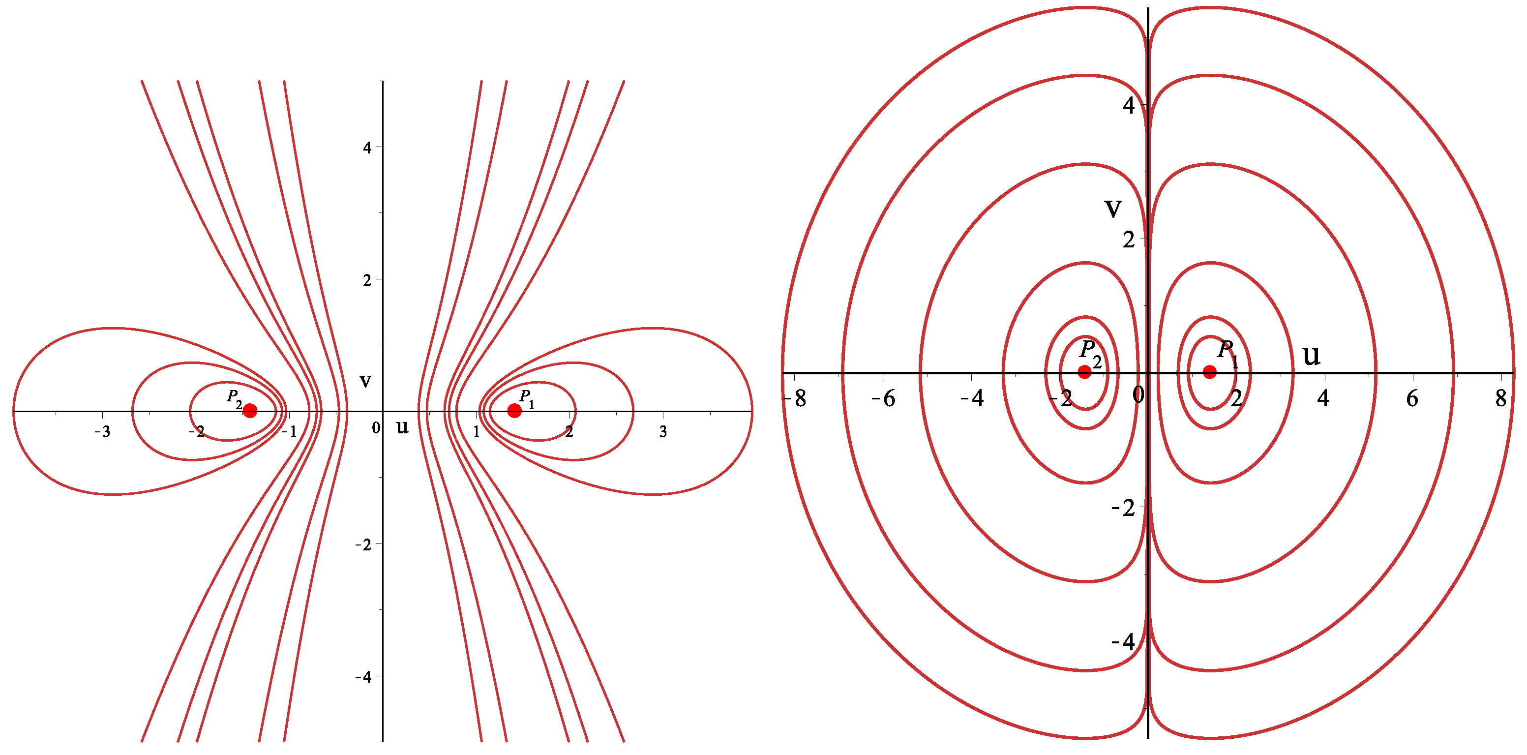
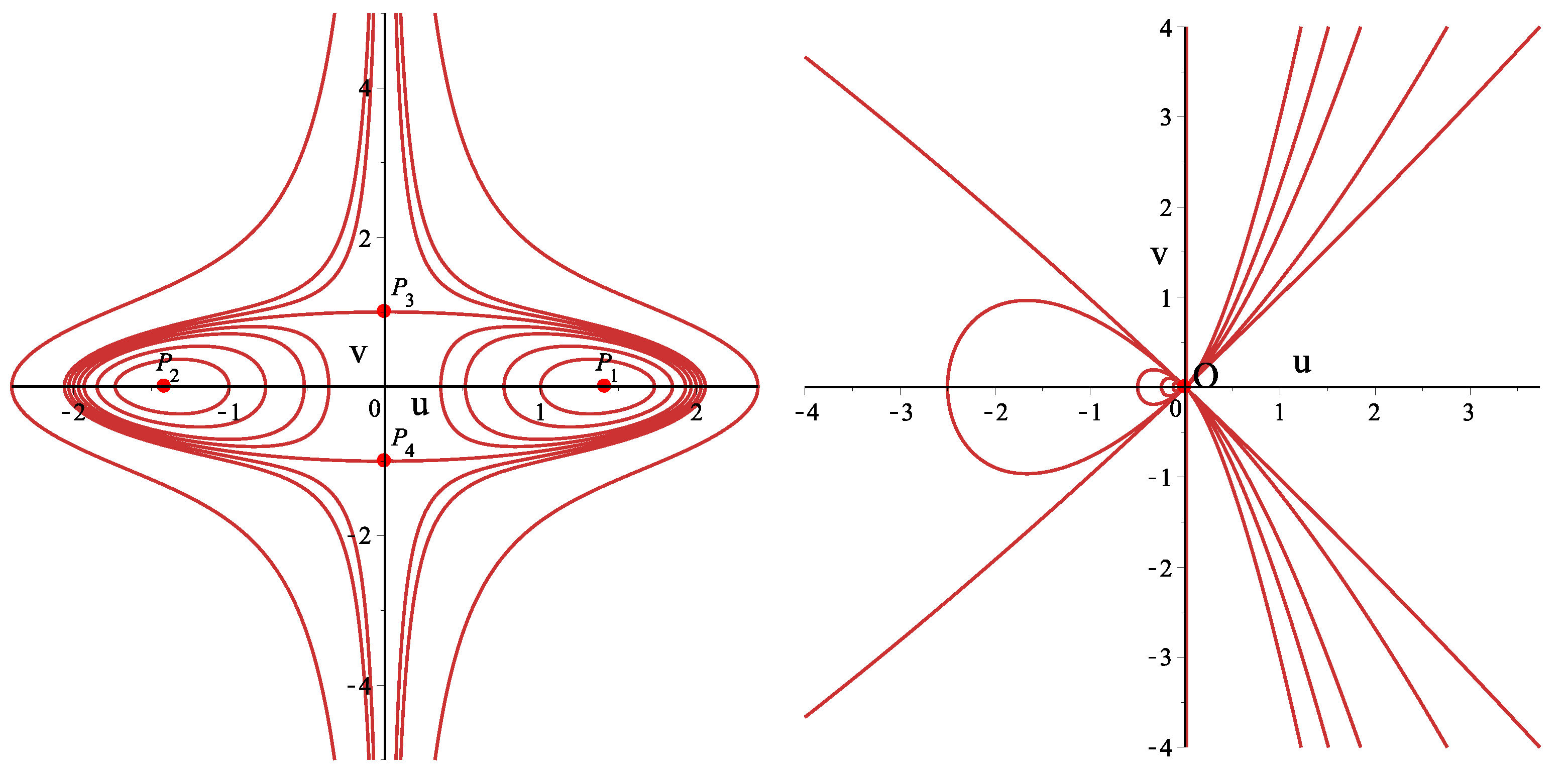
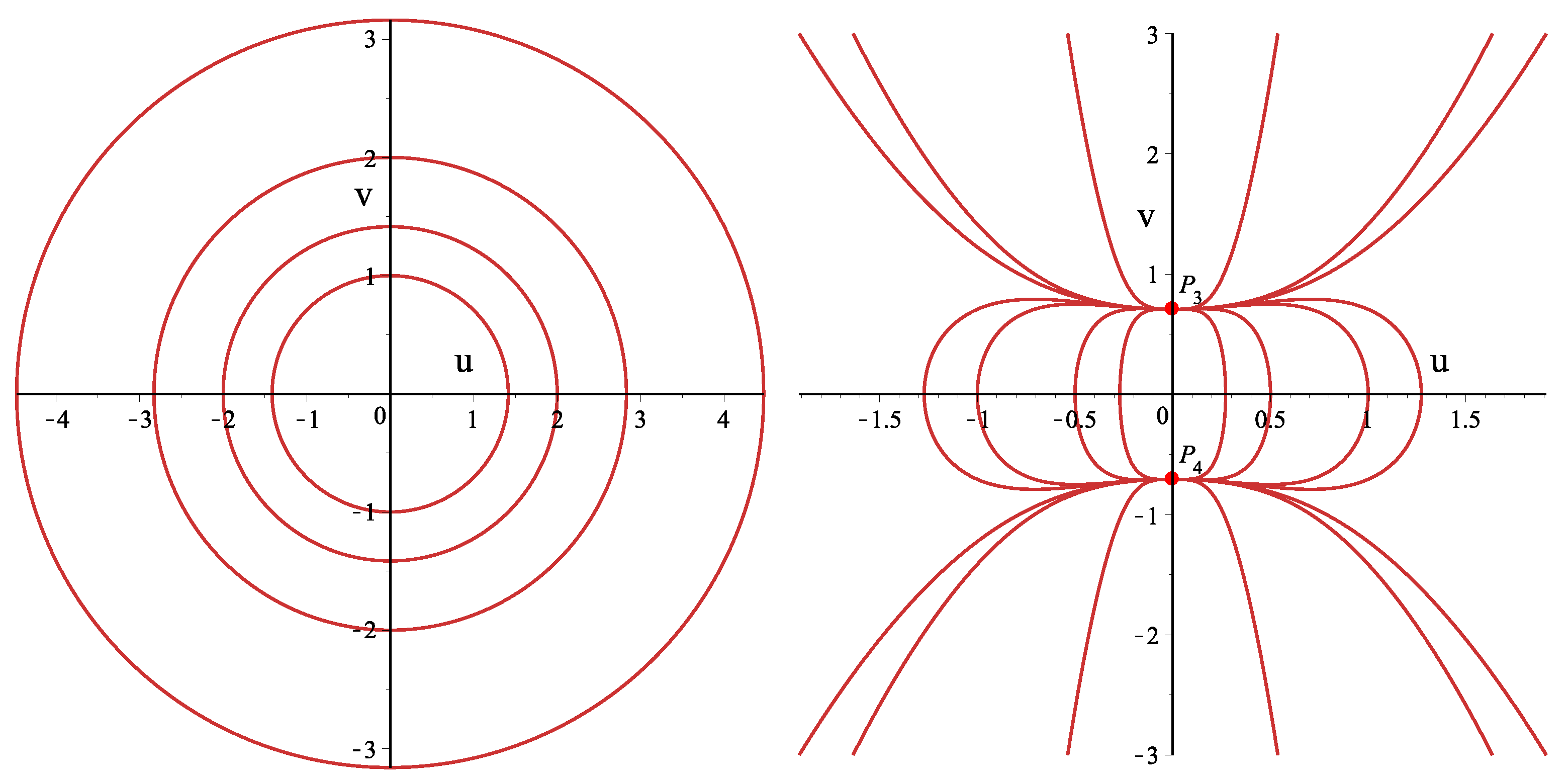
5. Phase-Plane Analysis of the Nonlinear Ordinary Differential Equations Corresponding to the Chavy–Waddy–Kolokolnikov Model

To visualize the results from the previous section, we analyse the stability of equilibrium points of (16) and explore the bifurcations of its phase portraits using the first integral obtained. Firstly, we rewrite (16) in the form

$$u_x=v, v_x=\frac{C_2-u^2+(\alpha +1)v^2}{2u}.$$

(21)

Letting $dx=2ud\xi$ gives the associated regular system [43] of (21) in the following form:

$$u_{\xi }=2uv, v_{\xi }=C_2-u^2+(\alpha +1)v^2.$$

(22)

The system of Equations (22) at $\alpha \ne 1$ and $\alpha \ne -1$ has the same first integral (20) as (21), which was found in the previous section:

$$H(u,v)=\frac{1}{4u^{\alpha +1}}\left({(\alpha -1)}^2{v}^2-(\alpha -1)u^2+\frac{C_2{(\alpha -1)}^2}{\alpha +1}\right).$$

The first integral of (22) for $\alpha =-1$ takes the form

$$H(u,v)=\frac{v^2}{2}+\frac{u^2}{4}-\frac{C_{2}ln\left|u\right|}{2}.$$

Systems (21) and (22) have the same orbits, for the exception of the neighbourhood of the straight line $u=0$. The vector field direction defined by the system (21) is changed to the inverse defined by (22), when the phase points intersect the singular straight line. Let us list all the possible equilibrium points of the regular system (22)

$$P_{1,2}=\pm (\sqrt{C_2},0), P_{3,4}=\left(0,\sqrt{-\frac{C_2}{\alpha +1}}\right), O=(0,0).$$

According to the theory of two-dimensional dynamical systems, the distributions and properties of the equilibrium points of (22) are as follows:

• When $C_2>0$ and $\alpha +1\ge 0$, the system (22) has two equilibrium points $P_{1,2}$, which are of the centre stability type. The solutions of the system in the vicinities of these equilibrium points are periodic (Figure 1 on the left- and right-hand sides).
• When $C_2>0$ and $\alpha +1<0$, the system (22) still has two centres $P_{1,2}$. Moreover, two saddle points $P_{3,4}$ appear. The solutions of the system (22) in the vicinities of the centres are periodic. The saddle points are connected to each other by the heteroclinic orbit (Figure 2 on the left-hand side).
• When $C_2=0$ and $\alpha +1\ne 0$, the centres $P_{1,2}$ and the saddle points $P_{3,4}$ vanish. The system (22) has one trivial equilibrium point O, which is degenerate with two zero eigenvalues. This point is connected to itself by the homoclinic orbit (Figure 2 on the right-hand side)
• When $C_2=0$ and $\alpha +1=0$, the system (22) has a line of equilibria $\{P=(0,v_0)| v_0\in \mathbb{R}\}$ which are linearly stable for $v_0<0$ and unstable for $v_0>0$. Each pair of points $P_v=(0,v)$ and $P_{-v}=(0,-v)$ are connected to each other by a heteroclinic orbit (Figure 3 on the left-hand side).
• When $C_2<0$ and $\alpha +1>0$, the system (22) has a pair of stable and unstable nodes $P_{3,4}$ (Figure 3 on the right-hand side). In this case, a saddle-node bifurcation for the equilibrium points $P_{3,4}$ occurs, as the value of $C_2$ decreases and crosses zero, while the value of $\alpha +1$ increases and crosses zero.
• When $C_2<0$ and $\alpha +1\le 0$, the nodes $P_{3,4}$ vanish, and system (22) does not have any equilibrium points.

This discussion above yields the bifurcations of the phase portraits of the regular system (22) as presented in Figure 1, Figure 2 and Figure 3. Corresponding to the phase portraits given are curves defined by $H(u,v)=h=const$ where h is varied. From the analysis of the first integral and the phase portraits, we can see that there exist bounded periodic solutions (Figure 1 and Figure 2 on the left-hand side and Figure 3 on the left-hand side) and solitary waves (Figure 2 on the right-hand side). In the next sections, we search explicit expressions for these orbits by means of various methods.

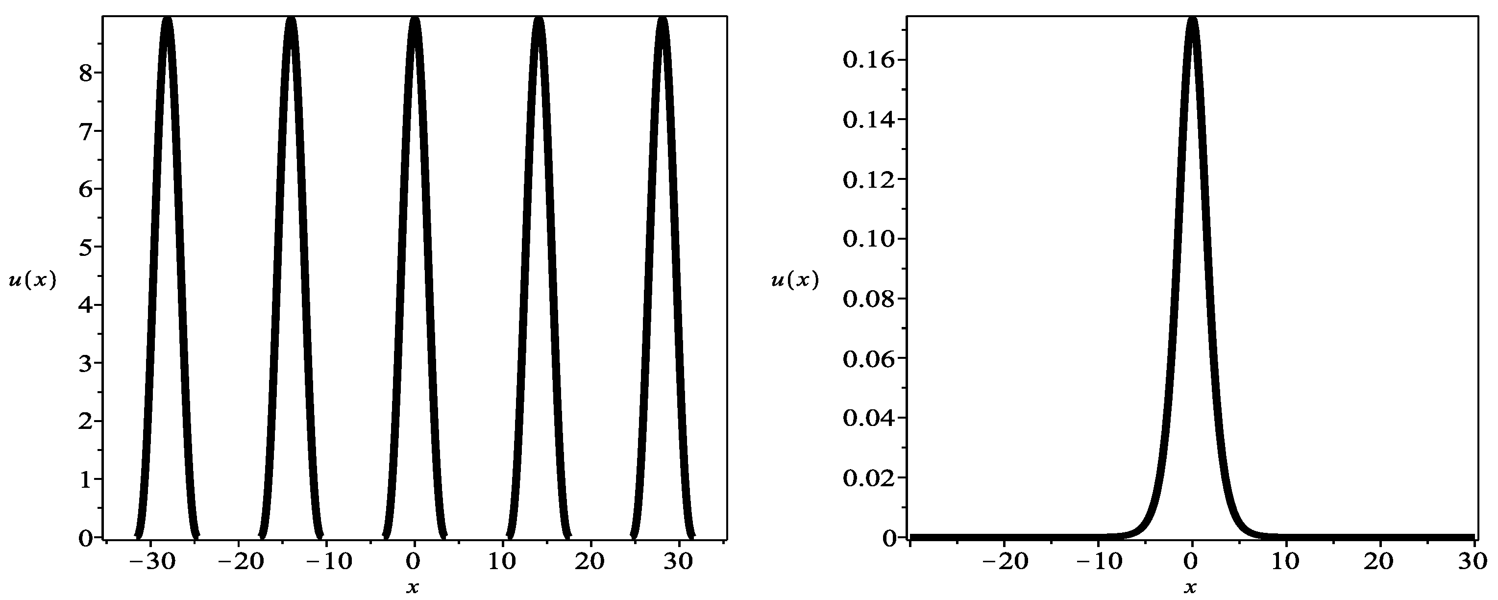
6. Stationary Solutions of the Chavy–Waddy–Kolokolnikov Model

Using the results from the previous sections, we can look for exact solutions of Equation (1). In this section, we find a number of new solutions of Equation (3) taking into account direct calculations.

In the case where $\alpha =3$, Equation (20) is written in the form

$$\begin{array}{c}{u}_x^2-C_3 u^4-\frac{1}{2} u^2+\frac{C_2}{4}=0.\end{array}$$

The solution of Equation (20) is expressed by the Jacobi elliptic function [40,41,44]

$$\begin{array}{c}u\left(x\right)=\sqrt{X_1} \mathrm{sn}\left\{\sqrt{C_3 X_2} (x-x_1), \frac{X_1}{X_2}\right\},\end{array}$$

where $x_1$ is an arbitrary constant, and $X_{1,2}$ solve the following algebraic equation

$$\begin{array}{c}{X}^2-\frac{1}{2 C_3} X+\frac{C_2}{4 C_3}=0,\end{array}$$

and have the form

$$\begin{array}{c}{X}_{1,2}=\frac{1\pm \sqrt{1-4 C_2 C_3}}{4 C_3}.\end{array}$$

Assuming $C_2=\frac{1}{4 C_3}$ yields $X_1=X_2$, so the solution $u\left(x\right)$ can be expressed by the formula [42,45,46]

$$\begin{array}{c}u\left(x\right)=\sqrt{C_3} tanh\left\{\sqrt{C_3} (x-x_1)\right\}.\end{array}$$

In the case where $C_2=0$ and $\alpha =3$, Equation (20) can be written as follows:

$$\begin{array}{c}{u}_x^2-\frac{1}{2} u^2-C_3 u^4=0.\end{array}$$

(23)

The solution of Equation (23) at $C_3<0$ is a solitary wave of the form (see [47])

$$\begin{array}{c}u\left(x\right)={\left[ {\mathrm{e}}^{\frac{x-x_1}{\sqrt{2}}}-\frac{C_3}{2} {\mathrm{e}}^{-\frac{x-x_1}{\sqrt{2}}} \right]}^{-1}.\end{array}$$

Assuming $\alpha =2$ in Equation (20), we obtain an equation of the form

$$\begin{array}{c}{u}_x^2-u^2-4 C_3 u^3+\frac{C_2}{3}=0.\end{array}$$

(24)

The general solution of Equation (24) is expressed via the Weierstrass elliptic function by the formula

$$\begin{array}{c}u\left(x\right)=\wp \left\{\sqrt{C_3} (x-x_2), g_2, g_3\right\}-\frac{1}{12 C_3},\end{array}$$

where the invariants $g_2$ and $g_3$ are as follows:

$$\begin{array}{c}{g}_2=\frac{1}{12C_3^2}, g_3=\frac{C_2}{3 C_3}-\frac{1}{216 C_3^3}.\end{array}$$

In the case where $C_2=0$ and $C_3\ne 0$, we obtain the solitary wave solution of Equation (24) in the form

$$\begin{array}{c}u\left(x\right)=\frac{1}{C_3}\left[{tanh}^2\left\{\frac{(x-x_2)}{2}\right\}-1\right].\end{array}$$

In the case where $\alpha =5$, Equation (20) is written as

$$\begin{array}{c}{u}_x^2-\frac{C_3}{4} u^6-\frac{1}{4} u^2+\frac{C_2}{6}=0.\end{array}$$

(25)

Introducing the following change of variables

$$\begin{array}{c}u\left(x\right)=\frac{1}{\sqrt{V\left(x\right)}}\end{array}$$

in Equation (25) yields

$$\begin{array}{c}{V}_x^2+\frac{2 C_2}{3} V^3-V^2-C_3=0,\end{array}$$

which has the general solution expressed by the formula [48]

$$\begin{array}{c}V\left(x\right)=\wp \left\{\sqrt{-\frac{C_2}{6}} (x-x_2), G_2, G_3\right\}+\frac{1}{2 C_2},\end{array}$$

where $\wp (z,G_2,G_3)$ is the Weierstrass elliptic function, $x_2$ is an arbitrary constant, and $G_2$, $G_3$ are the invariants of the form

$$\begin{array}{c}{G}_2=\frac{1}{2 C_2}, G_3=C_3+\frac{1}{6 C_2^2}.\end{array}$$

The stationary solution of Equation (1) at $\alpha =5$ is determined by the formula

$$\begin{array}{c}u\left(x\right)={\left[\wp \left\{\sqrt{-\frac{C_2}{6}} (x-x_2), g_2, g_3\right\}+\frac{1}{2 C_2}\right]}^{-\frac{1}{2}}.\end{array}$$

In fact, we can find a number of solutions of Equation (1) taking into account Equations (19) and (20). In particular, assuming $C_2=0$ in Equation (17), we obtain the general solution of the linear equation of the second order as follows:

$$\begin{array}{c}W\left(x\right)=C_4 exp\left\{\frac{\sqrt{\alpha -1}}{2} x\right\}+C_5 exp\left\{-\frac{\sqrt{\alpha -1}}{2} x\right\}\end{array}$$

and the stationary solution $u\left(x\right)$ given by

$$\begin{array}{c}u\left(x\right)={\left[C_4 exp\left\{\frac{\sqrt{\alpha -1}}{2} x\right\}+C_5 exp\left\{-\frac{\sqrt{\alpha -1}}{2} x\right\}\right]}^{\frac{2}{1-\alpha }}.\end{array}$$

(26)

At $\alpha >1$, the solution (26) describes the stationary solitary wave of Equation (1). The right-hand side of Figure 4 illustrates the stationary solitary wave of Equation (1). The left-hand side represents a periodic solution at $\alpha <1$.

At $C_3=0$, the solution of Equation (19) can be written as follows:

$$\begin{array}{c}W\left(x\right)={\left[\frac{4 ({\alpha }^2-1){\mathrm{e}}^{\frac{(x-x_3)}{\sqrt{\alpha -1}}}}{C_2 {(\alpha -1)}^3+4(\alpha +1){\mathrm{e}}^{\frac{2(x-x_3)}{\sqrt{\alpha -1}}}}\right]}^{\frac{\alpha -1}{2}},\end{array}$$

where $x_3$ is an arbitrary constant.

In the case where $C_2=0$, Equation (19) is expressed by

$$\begin{array}{c}{W}_x^2-\frac{(\alpha -1)}{4} W^2-C_3=0.\end{array}$$

(27)

The solution of Equation (27) is determined by the formulas

$$\begin{array}{c}W\left(x\right)=\frac{1}{2\sqrt{\alpha -1}}\left[exp\left\{\pm \frac{\sqrt{\alpha -1}}{2}(x-x_4)\right\}-4 C_3 exp\left\{\pm \frac{\sqrt{\alpha -1}}{2}(x-x_4)\right\}\right],\end{array}$$

where $x_4$ is an arbitrary constant.

Now, let us consider Equation (15) at $\alpha =1$ and $C_1=0$

$$\begin{array}{c}u u_{xxx}-u_x u_{xx}+u u_x=0.\end{array}$$

(28)

The first integral of Equation (28) can be written as follows:

$$\begin{array}{c}u u_{xx}-{u_x}^2+\frac{1}{2} u^2=C_6,\end{array}$$

where $C_6$ is an arbitrary constant.

At $C_6=0$, the solution of Equation (28) is expressed in the form of the solitary wave

$$\begin{array}{c}u\left(x\right)=C_7 exp\left\{-\frac{{(x-x_5)}^2}{4}\right\},\end{array}$$

where $C_7$ and $x_5$ are arbitrary constants.

7. Application of the Simplest Equation Method for Finding Exact Solutions of the Chavy–Waddy–Kolokolnikov Model

We can also find solutions of Equation (1) in the solitary wave form by applying the special method presented in the paper [42]. The essence of this method is that the solution is sought using lower-order equations. The Riccati equation or the equation for an elliptic function are usually taken as such simpler equations. Let us demonstrate this approach by looking for the solution of Equation (16) at $\alpha =\frac{3}{2}$.

The pole value of the general solution is $p=4$. Taking into account this value, we look for the solution of Equation (16) of the form (see [40,41,42,49,50,51,52,53,54,55,56,57,58,59,60,61,62,63,64,65,66,67,68])

$$\begin{array}{c}u\left(x\right)=A_0+A_1 Q\left(x\right)+A_2 Q{\left(x\right)}^2+A_3 Q{\left(x\right)}^3+A_4 Q{\left(x\right)}^4,\end{array}$$

(29)

where $A_j (j=0, 1, 2, 3, 4)$ are the unknown constants, and $Q\left(z\right)$ is a solution of the Riccati equation

$$\begin{array}{c}{Q}_x=k(Q^2-Q).\end{array}$$

(30)

The general solution of Equation (30) takes the form

$$\begin{array}{c}Q\left(x\right)=\frac{1}{1+exp\left\{k(x-z_1)\right\}},\end{array}$$

(31)

where $z_1$ is an arbitrary constant.

Solution (31) also solves the following nonlinear ordinary differential equation

$$\begin{array}{c}{Q}_x=2 k^2 Q^3-3 k^2 Q^2+k^2 Q.\end{array}$$

Substituting expression (29) into Equation (16) at $\alpha =\frac{3}{2}$, we obtain the polynomial in $Q\left(x\right)$. Equating the coefficients of this polynomial to zero and solving the resulting system of algebraic equations yields

$$\begin{array}{c}{A}_3=-2 A_4, A_2=\frac{\left(14 k^2-1\right)A_4}{12 k^2}, A_1=\frac{\left(2 k^2-1\right)A_4}{12 k^2},\\ A_0=-\frac{\left(4 k^4+20 k^2-11\right)A_4}{2880 k^4}, C_2=0,\\ k_{1,2}=\pm \frac{\sqrt{2}}{2}, k_{3,4,5,6}=\pm \frac{1}{20} \sqrt{-310\mp 30 i\sqrt{31}}.\end{array}$$

(32)

Taking into account expressions (32), we obtain the solitary wave solutions of Equation (16) at $C_2=0$. Two of these solutions are

$$\begin{array}{c}u\left(x\right)=\frac{A_4}{{\left(1+exp\left\{\frac{\sqrt{2}}{2} (x-z_1)\right\}\right)}^2}-\frac{2 A_4}{{\left(1+exp\left\{\frac{\sqrt{2}}{2} (x-z_1)\right\}\right)}^3}+\\ \frac{A_4}{{\left(1+exp\left\{\frac{\sqrt{2}}{2} (x-z_1)\right\}\right)}^4}.\end{array}$$

(33)

In the case where $\alpha =\frac{4}{3}$, we obtain $p=6$, and the solitary wave solution can be found as follows:

$$\begin{array}{c}u\left(x\right)=A_0+A_1 Q\left(x\right)+A_2 Q{\left(x\right)}^2+A_3 Q{\left(x\right)}^3+A_4 Q{\left(x\right)}^4+\\ +A_5 Q{\left(x\right)}^5+A_6 Q{\left(x\right)}^6,\end{array}$$

where $A_j (j=0, 1, 2, 3, 4, 5, 6)$ are constants, and $Q\left(z\right)$ is the solution of the Riccati Equation (30) as well.

Using the same algorithm, we obtain the following constraints:

$$\begin{array}{c}{A}_5=-3 A_6, A_4=\frac{\left(39 k^2-1\right)A_6}{12 k^2}, A_3=-\frac{\left(9 k^2-1\right)A_6}{6 k^2},\\ A_2=\frac{\left(279 k^4-105 k^2+4\right)A_6}{1080 k^4}, A_1=-\frac{\left(9 k^4-15 k^2+4\right)A_6}{1080 k^4},\\ A_0=\frac{\left(54 k^6+189 k^4+504 k^2-191\right)A_6}{1632960 k^6},\\ k_{1,2}=\pm \frac{\sqrt{3}}{3}, k_{3,4}=\pm \frac{i}{21}\sqrt{357}, k_{5,6,7,8}=\pm \frac{1}{3} \sqrt{\mp i\sqrt{26}-5}.\end{array}$$

The solitary wave solutions of Equation (16) at $k=k_{1,2}$ can be written as follows:

$$\begin{array}{c}u\left(x\right)=\frac{3 A_6}{{\left(1+{\mathrm{e}}^{\frac{\sqrt{3}}{3}\left(x-\mathit{x}\mathit{0}\right)}\right)}^4}-\frac{A_6}{{\left(1+{\mathrm{e}}^{\frac{\sqrt{3}}{3}\left(x-z_2\right)}\right)}^3}-\frac{3 A_6}{{\left(1+{\mathrm{e}}^{\frac{\sqrt{3}}{3}\left(x-z_2\right)}\right)}^5}+\\ \frac{A_6}{{\left(1+{\mathrm{e}}^{\frac{\sqrt{3}}{3}\left(x-z_2\right)}\right)}^6}.\end{array}$$

(34)

Assuming $\alpha =\frac{5}{4}$, we obtain the order of the pole $p=8$. In that case, the exact solution of Equation (15) at $C_1=0$ and (16) at $C_2=0$ can be found in the form

$$\begin{array}{c}u\left(x\right)=A_0+A_1 Q\left(x\right)+A_2 Q{\left(x\right)}^2+A_3 Q{\left(x\right)}^3+A_4 Q{\left(x\right)}^4+A_5 Q{\left(x\right)}^5+\\ A_6 Q{\left(x\right)}^6+A_7 Q{\left(x\right)}^7+A_8 Q{\left(x\right)}^8.\end{array}$$

By applying the same algorithm, we obtain the solitary wave solution as follows:

$$\begin{array}{c}u\left(x\right)=\frac{A_8}{{\left(1+{\mathrm{e}}^{\frac{1}{2}\left(x-x_0\right)}\right)}^4}-\frac{4 A_8}{{\left(1+{\mathrm{e}}^{\frac{1}{2}\left(x-x_0\right)}\right)}^5}+\frac{6 A_8}{{\left(1+{\mathrm{e}}^{\frac{1}{2}\left(x-x_0\right)}\right)}^6}-\\ \frac{4 A_8}{{\left(1+{\mathrm{e}}^{\frac{1}{2}\left(x-x_0\right)}\right)}^7}+\frac{A_8}{{\left(1+{\mathrm{e}}^{\frac{1}{2}\left(x-x_0\right)}\right)}^8}.\end{array}$$

(35)

One can note that using the binomial formula, we can present the solution (35) of Equation (15) as

$$\begin{array}{c}u\left(x\right)=\frac{A_8}{{\left(1+{\mathrm{e}}^{\frac{x-x_0}{2}}\right)}^4} {\left(1-\frac{1}{1+{\mathrm{e}}^{\frac{x-x_0}{2}}}\right)}^4.\end{array}$$

(36)

The solutions (33) and (34) can also be written in such a form. This observation suggests that the solution of Equations (15) and (16) can be found in the form

$$\begin{array}{c}u\left(x\right)=\frac{C {\mathrm{e}}^{\frac{(x-x_0)}{\sqrt{\alpha -1}}}}{{\left(1+{\mathrm{e}}^{\sqrt{\alpha -1}(x-x_0)}\right)}^{\frac{2}{\alpha -1}}},\end{array}$$

(37)

where C and $x_0$ are arbitrary constants. Solution (37) satisfies Equation (15) at $C_1=0$ and (16) at $C_2=0$ for arbitrary values of parameter $\alpha$. This solution is similar to solution (26) of Equation (1). In Section 2, we obtained, that Equation (15) passed the Painlevé test at $C_0=0$ and $C_1=0$ in the case where $\alpha =1+\frac{N_2}{N_1}$, where $N_1\in \mathbb{N}$ and $N_2\in \mathbb{N}$. However, we can see that there exist analytical solutions (26) and (37) of Equation (1) at an arbitrary value of the parameter $\alpha$, which are expressed by the multifunction.

8. Conclusions

In this article, the Chavy–Waddy–Kolokolnikov mathematical model for the description of bacterial density, which consists of a fourth-order partial differential Equation (1), was investigated. The major focus of this work was to look for possible analytical solutions to Equation (1). For this purpose, we carried out the Painlevé test to determine the integrability of the mathematical model. Applying the Painlevé test to a nonlinear ordinary differential equation obtained from the original Chavy–Waddy–Kolokolnikov mathematical model allowed us to establish that the Cauchy problem for a partial differential equation could not be solved by the method of the inverse scattering transform, so the original equation was not integrable. Using the Painlevé test, we found the conditions for the parameter of the mathematical model $\alpha$ under which stationary analytical solutions of the Chavy–Waddy–Kolokolnikov equation could be found. In this work, for the first time, the first integral of a nonlinear ordinary differential equation corresponding to the original mathematical model was obtained and a classification of the phase portraits of the corresponding dynamical system was given, which illustrated the possibility of finding stationary bounded analytical solutions. By means of direct transformations, stationary analytical solutions to the nonlinear Chavy–Waddy–Kolokolnikov partial differential equation were obtained for various parameter values of the mathematical model. The application of the method of simplest equations for constructing analytical solutions of the stationary equation made it possible to find analytical solutions for integer values of the model parameter. However, using the Newton binomial formula, partial sums were presented as a formula for an arbitrary parameter $\alpha$ of the mathematical model.

References

1. Keller, E.F.; Segel, L.A. Traveling bands of chemotactic bacteria: A theoretical analysis. J. Theor. Biol. 1971, 30, 235–248. [Google Scholar] [CrossRef] [PubMed]
2. Keller, E.F.; Segel, L.A. Model for chemotaxis. J. Theor. Biol. 1971, 30, 225–234. [Google Scholar] [CrossRef] [PubMed]
3. Keller, E.F.; Segel, L.A. Initiation of slime mold aggregation viewed as an instability. J. Theor. Biol. 1970, 26, 399–415. [Google Scholar] [CrossRef]
4. Liu, P.; Shi, J.; Wang, Z.-A. Pattern formation of the attraction-repulsion Keller-Segel system. Discret. Contin. Dyn. Syst.-B 2013, 18, 2597. [Google Scholar] [CrossRef]
5. Winkler, M. Finite-time blow-up in the higher-dimensional parabolic–parabolic Keller-Segel system. J. Math. Pures Appl. 2013, 100, 748–767. [Google Scholar] [CrossRef]
6. Arumugam, G.; Tyagi, J. Keller-Segel chemotaxis models: A review. Acta Appl. Math. 2021, 171, 6. [Google Scholar] [CrossRef]
7. Horstmann, D. From 1970 until Present: The Keller-Segel Model in Chemotaxis and Its Consequences. Jahresberichte DMV 2003, 105, 103–165. [Google Scholar]
8. Wang, Z.; Thomas, H. Classical solutions and pattern formation for a volume filling chemotaxis model. Chaos Interdiscip. J. Nonlinear Sci. 2007, 17, 037108. [Google Scholar] [CrossRef]
9. Iglesias, P.A.; Devreotes, P.N. Navigating through models of chemotaxis. Curr. Opin. Cell Biol. 2008, 20, 35–40. [Google Scholar] [CrossRef]
10. Burkart, U.; Häder, D.P. Phototactic attraction in light trap experiments: A mathematical model. J. Math. Biol. 1980, 10, 257–269. [Google Scholar] [CrossRef]
11. Marée, A.F.M.; Panfilov, A.V.; Hogeweg, P. Phototaxis during the slug stage of Dictyostelium discoideum: A model study. Proc. R. Soc. Lond. Ser. B Biol. Sci. 1999, 266, 1351–1360. [Google Scholar] [CrossRef]
12. Bhaya, D.; Levy, D.; Requeijo, T. Group dynamics of phototaxis: Interacting stochastic many-particle systems and their continuum limit. In Hyperbolic Problems: Theory, Numerics, Applications; Springer: Berlin/Heidelberg, Germany, 2008. [Google Scholar]
13. Levy, D.; Requeijo, T. Stochastic models for phototaxis. Bull. Math. Biol. 2008, 70, 1684–1706. [Google Scholar] [CrossRef]
14. Levy, D.; Requeijo, T. Modeling group dynamics of phototaxis: From particle systems to PDEs. Discret. Contin. Dyn. Syst. Ser. B 2008, 9, 103. [Google Scholar] [CrossRef]
15. Galante, A.; Levy, D. Modeling selective local interactions with memory. Phys. D Nonlinear Phenom. 2013, 260, 176–190. [Google Scholar] [CrossRef] [Green Version]
16. Weinberg, D.; Levy, D. Modeling selective local interactions with memory: Motion on a 2D lattice. Phys. D Nonlinear Phenom. 2014, 278, 13–30. [Google Scholar] [CrossRef] [Green Version]
17. Bhaya, D. Light matters: Phototaxis and signal transduction in unicellular cyanobacteria. Mol. Microbiol. 2004, 53, 745–754. [Google Scholar] [CrossRef] [PubMed]
18. Burriesci, M.; Bhaya, D. Tracking phototactic responses and modeling motility of Synechocystis sp. strain PCC6803. J. Photochem. Photobiol. B Biol. 2008, 91, 77–86. [Google Scholar] [CrossRef]
19. Samuel, S.; Gill, V. Diffusion-chemotaxis model of effects of cortisol on immune response to human immunodeficiency virus. Nonlinear Eng. 2018, 7, 207–227. [Google Scholar] [CrossRef]
20. Chaplain, M.A.J.; Lolas, G. Mathematical modelling of cancer cell invasion of tissue: The role of the urokinase plasminogen activation system. Math. Models Methods Appl. Sci. 2005, 15, 1685–1734. [Google Scholar] [CrossRef] [Green Version]
21. Chaplain, M.A.J.; Lolas, G. Mathematical modelling of cancer invasion of tissue: Dynamic heterogeneity. Netw. Heterog. Media 2006, 1, 399–439. [Google Scholar] [CrossRef]
22. Faraz, N.; Khan, Y.; Goufo, E.D.; Anjum, A.; Anjum, A. Dynamic analysis of the mathematical model of COVID-19 with demographic effects. Z. Naturforschung C 2020, 75, 389–396. [Google Scholar] [CrossRef] [PubMed]
23. Ayers, K.L.; Eggers, S.; Rollo, B.N.; Smith, K.R.; Davidson, N.M.; Siddall, N.A.; Zhao, L.; Bowles, J.; Weiss, K.; Zanni, G.; et al. Variants in SART3 cause a spliceosomopathy characterised by failure of testis development and neuronal defects. Nat. Commun. 2023, 14, 3403. [Google Scholar] [CrossRef] [PubMed]
24. Ooka, H.; Ishii, T.; Hashimoto, K.; Nakamura, R. Light-induced cell aggregation of Euglena gracilis towards economically feasible biofuel production. RSC Adv. 2014, 4, 20693–20698. [Google Scholar] [CrossRef]
25. Itoh, A. Euglena Motion Control by Local Illumination. In Bio-Mechanisms of Swimming and Flying; Springer: Tokyo, Japan, 2004. [Google Scholar]
26. Itoh, A.; Tamura, W. Object manipulation by a formation-controlled Euglena group. In Bio-Mechanisms of Swimming and Flying: Fluid Dynamics, Biomimetic Robots, and Sports Science; Springer: Tokyo, Japan, 2008. [Google Scholar]
27. Chavy-Waddy, P.-C.; Kolokolnikov, T. A local PDE model of aggregation formation in bacterial colonies. Nonlinearity 2016, 29, 3174–3185. [Google Scholar] [CrossRef] [Green Version]
28. Leon-Ramírez, A.; Gonzalez-Gaxiola, O.; Chacon-Acosta, G. Analytical Solutions to the Chavy-Waddy-Kolokolnikov Model of Bacterial Aggregates in Phototaxis by Three Integration Schemes. Mathematics 2023, 11, 2352. [Google Scholar] [CrossRef]
29. Painlevé, P. Sur les equations differentielles du second ordre et d’ordre superieur dont l’integrale generale est uniforme. Acta Math. 1902, 25, 1–85. [Google Scholar] [CrossRef]
30. Gambier, B. Sur les équations différetielles dont l’integrate générale est uniforme. C. R. Acad. Sc. Paris 1906, 142, 1403–1406+1497–1500. [Google Scholar]
31. Ince, E.L. Ordinary Differential Equations; Dover Publishing, Inc.: New York, NY, USA, 1956. [Google Scholar]
32. Ablowitz, M.J.; Ramani, A.; Segur, H. Nonlinear evolution equations and ordinary differential equations of Painlevé type. Lett. Nuovo C. 1978, 23, 333–338. [Google Scholar] [CrossRef]
33. Ablowitz, M.J.; Ramani, A.; Segur, H. A connection between nonlinear evolution equations and ordinary differential equations of P-type. I. J. Math. Phys. 1979, 21, 715–721. [Google Scholar] [CrossRef]
34. Ablowitz, M.J.; Ramani, A.; Segur, H. A connection between nonlinear evolution equations and ordinary differential equations of P-type. II. J. Math. Phys. 1979, 21, 1006–1015. [Google Scholar] [CrossRef]
35. Kudryashov, N.A. Painlevé analysis and exact solutions of the Korteweg-de Vries equation with a source. Appl. Math. Lett. 2015, 41, 41–45. [Google Scholar] [CrossRef]
36. Kudryashov, N.A. The generalized Duffing oscillator. Commun. Nonlinear Sci. Numer. Simul. 2021, 93, 105526. [Google Scholar] [CrossRef]
37. Kudryashov, N.A. Exact solutions of the equation for surface waves in a convecting fluid. Appl. Math. Comput. 2019, 344–345, 97–106. [Google Scholar] [CrossRef]
38. Davis, H.T. Introduction to Nonlinear Differential and Integral Equations; US Atomic Energy Commission: Washington, DC, USA, 1960.
39. Kudryashov, N.A. Exact solutions of the complex Ginzburg-Landau equation with law of four powers of nonlinearity. Optik 2022, 265, 169548. [Google Scholar] [CrossRef]
40. Kudryashov, N.A. Method for finding highly dispersive optical solitons of nonlinear differential equations. Optik 2020, 206, 163550. [Google Scholar] [CrossRef]
41. Kudryashov, N.A. Mathematical model of propagation pulse in optical fiber with power nonlinearities. Optik 2020, 212, 164750. [Google Scholar] [CrossRef]
42. Kudryashov, N.A. One method for finding exact solutions of nonlinear differential equations. Commun. Nonlinear Sci. Numer. Simul. 2012, 17, 2248–2253. [Google Scholar] [CrossRef] [Green Version]
43. Li, J.; Guanrong, C. On a class of singular nonlinear traveling wave equations. Int. J. Bifurc. Chaos 2007, 17, 4049–4065. [Google Scholar] [CrossRef]
44. Jacobi, C.G.J. Jacobi: Fundamenta Nova Theoriae Functionum Ellipticarum; Bornträger: Kenigsberg, Russia, 1829. [Google Scholar]
45. Kudryashov, N.A. Solitary wave solutions of hierarchy with non-local nonlinearity. Appl. Math. Lett. 2020, 103, 106155. [Google Scholar] [CrossRef]
46. Whittaker, E.T.; Watson, G.N. A Course of Modern Analysis; Cambridge University Press: Cambridge, UK, 1927. [Google Scholar]
47. Kudryashov, N.A. A generalized model for description of propagation pulses in optical fiber. Optik 2019, 189, 42–52. [Google Scholar] [CrossRef]
48. Akhiezer, N.I. Elements of the Theory of Elliptic Functions; AMS: Providence, RI, USA, 1990; Volume 79, ISBN 0-8218-4532-2. [Google Scholar]
49. Kudryashov, N.A. Implicit solitary waves for one of the generalized nonlinear Schrödinger equations. Mathematics 2021, 9, 3024. [Google Scholar] [CrossRef]
50. Kudryashov, N.A. Optical solitons of the generalized nonlinear Schrödinger equation with Kerr nonlinearity and dispersion of unrestricted order. Mathematics 2022, 10, 3409. [Google Scholar] [CrossRef]
51. Akbulut, A. Obtaining the Soliton Type Solutions of the Conformable Time-Fractional Complex Ginzburg-Landau Equation with Kerr Law Nonlinearity by Using Two Kinds of Kudryashov Methods. J. Math. 2023, 2023, 4741219. [Google Scholar] [CrossRef]
52. Onder, I.; Secer, A.; Bayram, M. Optical soliton solutions of time-fractional coupled nonlinear Schrodinger system via Kudryashov-based methods. Optik 2023, 272, 170362. [Google Scholar] [CrossRef]
53. Cakicioglu, H.; Ozisik, M.; Secer, A.; Bayram, M. Optical soliton solutions of Schrodinger-Hirota equation with parabolic law nonlinearity via generalized Kudryashov algorithm. Opt. Quantum Electron. 2023, 55, 407. [Google Scholar] [CrossRef]
54. Albayrak, P. Optical solitons of Biswas-Milovic model having spatio-temporal dispersion and parabolic law via a couple of Kudryashov’s schemes. Optik 2023, 279, 170761. [Google Scholar] [CrossRef]
55. Cinar, M.; Secer, A.; Ozisik, M.; Bayram, M. Optical soliton solutions of (1 + 1)-and (2 + 1)-dimensional generalized Sasa-Satsuma equations using new Kudryashov method. Int. J. Geom. Methods Mod. Phys. 2023, 20, 2350034. [Google Scholar] [CrossRef]
56. Ozisik, M.; Secer, A.; Bayram, M. On the investigation of chiral solitons via modified new Kudryashov method. Int. J. Geom. Methods Mod. Phys. 2023, 17, 23501. [Google Scholar] [CrossRef]
57. Malik, S.; Hashemi, M.S.; Kumar, S.; Rezazadeh, H.; Mahmoud, W.; Osman, M.S. Application of new Kudryashov method to various nonlinear partial differential equations. Opt. Quantum Electron. 2023, 55, 8. [Google Scholar] [CrossRef]
58. Ozisik, M.; Secer, A.; Bayram, M.; Sulaiman, T.A.; Yusuf, A. Acquiring the solitons of inhomogeneous Murnaghan’s rod using extended Kudryashov method with BernoulliRiccati approach. Int. J. Mod. Phys. B 2022, 36, 2250221. [Google Scholar] [CrossRef]
59. Akbar, M.A.; Wazwaz, A.M.; Mahmud, F.; Baleanu, D.; Roy, R.; Barman, H.K.; Mahmoud, W.; Al Sharif, M.A.; Osman, M.S. Dynamical behavior of solitons of the perturbed nonlinear Schrodinger equation and microtubules through the generalized Kudryashov scheme. Results Phys. 2022, 43, 106079. [Google Scholar] [CrossRef]
60. Kumar, S.; Niwas, M. New optical soliton solutions of Biswas-Arshed equation using the generalised exponential rational function approach and Kudryashov’s simplest equation approach. Pramana J. Phys. 2022, 96, 204. [Google Scholar] [CrossRef]
61. Esen, H.; Secer, A.; Ozisik, M.; Bayram, M. Soliton solutions to the nonlinear higher dimensional Kadomtsev-Petviashvili equation through the new Kudryashov’s technique. Phys. Scr. 2022, 97, 115104. [Google Scholar] [CrossRef]
62. Wang, X.; Akram, G.; Sadaf, M.; Mariyam, H.; Abbas, M. Soliton Solution of the Peyrard-Bishop-Dauxois Model of DNA Dynamics with M-Truncated and β-Fractional Derivatives Using Kudryashov-s R Function Method. Fractal Fract. 2022, 6, 616. [Google Scholar] [CrossRef]
63. Ozisik, M.; Secer, A.; Bayram, M.; Aydin, H. An encyclopedia of Kudryashov’s integrability approaches applicable to optoelectronic devices. Optik 2022, 265, 169499. [Google Scholar] [CrossRef]
64. Arnous, A.H.; Biswas, A.; Kara, A.H.; Milovic, D.; Yildirim, Y.; Alshehri, H.M. Sequel to cubic-quartic optical soliton perturbation with complex Ginzburg-Landau equation by the enhanced Kudryashov’s method. IET Optoelectron. 2022, 16, 149–159. [Google Scholar] [CrossRef]
65. Ionescu, C.; Babalic, C.N.; Constantinescu, R.; Efrem, R. The Functional Expansion Approach for Solving NPDEs as a Generalization of the Kudryashov and G′/G Methods. Symmetry 2022, 14, 827. [Google Scholar] [CrossRef]
66. Arnous, A.H.; Biswas, A.; Yildirim, Y.; Zhou, Q.; Liu, W.; Alshomrani, A.S.; Alshehri, H.M. Cubic-quartic optical soliton perturbation with complex Ginzburg-Landau equation by the enhanced Kudryashov’s method. Chaos Solitons Fractals 2022, 155, 111748. [Google Scholar] [CrossRef]
67. Arnous, A.H.; Zhou, Q.; Biswas, A.; Guggilla, P.; Khan, S.; Yildirim, Y.; Alshomrani, A.S.; Alshehri, H.M. Optical solitons in fiber Bragg gratings with cubic-quartic dispersive reflectivity by enhanced Kudryashov’s approach. Phys. Lett. Sect. A Gen. At. Solid State Phys. 2022, 422, 127797. [Google Scholar] [CrossRef]
68. Tekercioglu, R. On TheE Traveling Wave Solutions of Pulse Propagation in Monomode Fiber via the extended Kudryashov’s Approach. Therm. Sci. 2022, 26, S49–S59. [Google Scholar] [CrossRef]
Figure 1. Phase portraits of (16) for α = 3 ,   C 2 = 2 (left-hand side) and α = 1 ,   C 2 = 2 (right-hand side).
Mathematics 11 03203 g001
Figure 2. Phase portraits of (16) for α = 3 ,   C 2 = 2 (left-hand side) and α = 3 ,   C 2 = 0 (right-hand side).
Mathematics 11 03203 g002
Figure 3. Phase portraits of (16) for α = 1 ,   C 2 = 0 (left-hand side) and α = 3 ,   C 2 = 2 (right-hand side).
Mathematics 11 03203 g003
Figure 4. The real part of the stationary solution (26) of Equation (1) at α = 0.2 , C 4 = 1.2 and C 5   = 1.2 (left-hand side) and the function (26) of Equation (1) at α = 2.0 , C 4 = 1.2 and C 5 = 1.2 (right-hand side).
Mathematics 11 03203 g004
Disclaimer/Publisher’s Note: The statements, opinions and data contained in all publications are solely those of the individual author(s) and contributor(s) and not of MDPI and/or the editor(s). MDPI and/or the editor(s) disclaim responsibility for any injury to people or property resulting from any ideas, methods, instructions or products referred to in the content.