1. Introduction
Oil fields with a gas cap comprise a significant proportion of gas and oil fields [
1]. Oil production from such deposits has specific characteristics and differs from the development of pure oil deposits [
2]. A decrease in pressure in the oil-saturated region causes movement of the gas–oil contact surface. It may be unstable and lead to gas breakdown in the production well. As a result, residual oil is formed in the reservoir [
3]. In addition, the instability and breakdown of gas–oil and water–oil surfaces can lead to discontinuity and fragmentation of the oil flow, which also causes the formation of residual oil in the field [
4].
Displacing oil from the reservoir by gas is an effective method for increasing oil recovery [
5]. The process is more efficient if water displacement is injected first, then gas. In this case, gas and oil are separated by a layer of water, and both the water–gas and water–oil boundaries are unstable. Carbon dioxide is injected into depleted oil reservoirs for storage purposes to reduce climatic impacts and improve oil recovery [
6]. In this process, gas is often injected into a porous medium filled with water and oil. Thus, studying the evolution of the water–gas and water–oil interfaces and the mutual influence of these processes is an important task.
Recently, analytical and numerical studies have been carried out on the instability of the interface boundary during filtration in soils and rocks [
7]. It was found that in many cases, important for applications, the transition to instability occurs for all values of the wave number simultaneously or at infinitely large wave numbers [
7]. The fastest-growing mode of the unsteady flow is the mode corresponding to an infinitesimal linear size. Finding the parameters of the fastest-growing perturbation is of interest for determining the characteristic scale of the resulting finger-like structures, the decay of which leads to volumes of liquid. In the classical work [
8], the problem of the instability of the displacement of a more viscous liquid by a less viscous one was considered. The transition to instability occurred simultaneously at all wave numbers, which did not make it possible to establish the characteristic size of the most unstable perturbation. In [
9], the stability of the gas–oil interface in a gas cap under a pressure drop in the oil-saturated region was studied. A criterion for surface stability was found, showing that when the parameters change, the transition to the unstable regime is also realized simultaneously at all wave numbers.
However, it was shown in [
10] that anomalous short-wave instability does not occur if the Brinkman equation is used instead of Darcy’s law. Using the normal mode method, it was found that the growth rate of small perturbations of the liquid–gas surface tends to zero with increasing wave number. An extensive review of experimental studies of three-phase relative permeability is presented in [
11]. The results of a pore-scale experimental survey of a two-phase oil/brine flow through a miniature, water-wet fractured sandstone core sample were presented in [
12].
There are several approaches to studying the process of liquid displacement by gas. In the piston model (continuum single-phase model) of displacement, it is assumed that there is either gas, water, or oil at each point of the medium. In this case, it is assumed that there is a boundary between different liquids, as well as between a liquid and a gas, which, in a large-scale approximation, represents a moving surface. This model was used to study the main features of the development of instability in many works (see, for example, Ref. [
13] and the review in [
14]). The problem of the displacement of one incompressible fluid by another in an inhomogeneous layered porous medium was also studied in [
15]. In this case, it was assumed that the injected fluid completely displaces the previously filling fluid, and there is a moving interface between them.
Using the three-phase continuum approach, three phases (water, oil and gas) are expected to coexist at every point in the porous medium when viewed from a macroscopic point of view (see, for example, Refs. [
16,
17] and a detailed review in [
18]). General analytical solutions for a three-phase immiscible flow in a one-dimensional porous medium with concave relative permeability curves are presented in [
19].
Along with the continuum approximation, network models are used to study oil displacement processes [
20]. The network model allows us to take into account processes occurring at the micro level. Thus, it is assumed that water, oil and gas flow in close but different channels or are separated within each. For example, in [
21], the process of the displacement of oil from the reservoir by gas is considered. It is assumed that gas, water and oil formally exist at every point in the medium at the macro level, but at the micro level, they are located in separate, closely spaced pores. In [
22], drainage displacements in a three-phase flow under strongly wetting conditions are described by the pore-scale network model. In [
23], the oil and gas outflow process is also described using a three-dimensional network model. Agreement between the calculated and experimental data was obtained.
It is important to note that there is a problem of sediment formation when water is injected into the reservoir. Asphaltenes possess the ability to accumulate at the interface of oil and water, leading to the formation of stable emulsions. An experimental investigation of this phenomena is presented in [
24]. Molecular dynamics simulations are developed in [
24]. The effect of ions in water on asphaltene aggregation was studied in [
25]. The influence of water cut on the effectiveness of an asphaltene inhibitor was investigated in [
26].
An interesting and promising approach is a combined multiphase lattice Boltzmann color-gradient model for simulating the flow of immiscible two- and three-phase liquids (see, for example, Ref. [
6]). In [
9], a single-phase continuum model was used to study the development of gas–liquid interface instability in a porous medium. It is shown that at the initial stage of the development of a perturbation, the results obtained by the normal mode method for linearized equations of a single-phase continuum model are consistent with the solution of the nonlinear problem. At the same time, using the network model makes it possible to obtain qualitative results that are consistent with the single-phase continuum model results.
In this paper, a single-phase continuum model is used to describe the evolution of gas–water and water–oil interface perturbations. The main novelty of this work is that analytical solutions have been obtained that describe the main patterns of the mutual influence of the development of disturbances at the water–gas and water–oil boundaries.
The paper is organized as follows:
Section 2 contains the formulation of the problem within the continuum model using Darcy’s law. The specific boundary conditions are given. Next, the governing equations and the boundary conditions are made dimensionless. In
Section 3, a vertical flow solution is obtained for the stability study. The water–gas and water–oil interfaces are initially assumed to be flat. Time-dependent pressure and velocity profiles are obtained. In
Section 4, a linear stability analysis of the basic solution is presented. The governing equations and boundary conditions are linearized about the basic solution. According to the classical procedure, the normal mode method is used to study the behaviour of the perturbed interfaces. The problem of the evolution of infinitesimal perturbations of gas–water and oil–water surfaces is solved in a linear approximation, taking into account their mutual influence.
Section 5 contains a discussion of the results obtained. In the conclusion, the main results of the work are summarized.
Appendix A contains a derivation of approximate formulas for large and small values of the dimensionless wave number.
2. Formulation of the Problem
We consider water and oil filtration in a horizontal layer of porous medium (
Figure 1). Region 0 is filled with gas. The pressure in this region is assumed to be constant and equal to
. Region 1 is filled with water with parameters
and
of viscosity and density, respectively. There exists a water–gas interface that separates the water from the gas. A continuous pressure at this interface is prescribed. At the lower boundary, region 1 is in contact with layer 2, which is oil-saturated with the corresponding viscosity and density parameters
and
. The
-coordinates of the gas–water and water–oil interfaces are described by the functions
and
, respectively. Regions 0, 1 and 2 are located inside a relatively low-permeability porous medium layer. Region 3 contains a highly permeable layer modelling a horizontal well or fracture with constant pressure,
.
The fluids are assumed to be incompressible, and the filtration flow is described by Darcy’s equation [
27]:
where
is the filtration velocity,
is the pressure,
is the density,
is the acceleration due to gravity,
is the viscosity,
is the permeability and the subscripts 1 and 2 correspond to the water and oil regions, respectively.
According to [
27], we solve these equations subject to the boundary conditions of constant pressure on the gas–water interface and on the lower boundary of region 2. In addition, the flow fields in layers 1 and 2 (see
Figure 1) are coupled by the requirements of pressure continuity across the water–oil interface and no flow through this interface. The pressure continuity condition neglects the effect of capillary pressure because the general question of the stability or instability of the interfaces is independent of the inclusion of this phenomenon [
27].
The boundary condition at the gas–water interface (
) is
The pressure is equal to
at the lower boundary of the region saturated with oil. The corresponding boundary condition can be written as
If the pressure and the normal component of velocity at the water–oil interface (
) are continuous, then we obtain
where
The evolution of the interfaces between gas and water and water and oil is described by the equations
Equations (
7) and (
8) will be used in the form
where
The governing equations and the boundary conditions are made dimensionless using the following reference parameters
where
is characteristic pressure,
is characteristic size and
is characteristic velocity.
The governing equations and the boundary conditions, using the normalised quantities (
12), take the form
4. Evolution of Infinitesimal Perturbations of Vertical Flow
We now consider the stability of the solution (
29)–(
31) to infinitesimal perturbations derived in the previous section. An infinitesimal perturbation is applied to the basic flow to examine the stability of the interfaces. The aim is to linearise the governing equations and boundary conditions about the basic solution (
29)–(
31) and to study the behaviour of the perturbed interfaces. The velocity and pressure fields both in the water and oil regions and the interface positions are expanded in the following manner:
where
,
,
,
,
,
,
and
are small perturbations of the positions of the gas–water and water–oil interfaces, the pressure, and the horizontal and vertical components of the filtration velocity in the regions filled with water and oil, respectively.
Let us obtain the basic equations of the problem in a linearized form. We substitute the expressions (
42)–(
49) into the system of Equations (13):
The boundary conditions are
The system of equations for perturbations has the form
and the boundary conditions expressed as:
We assume that the solutions for
,
,
and
have the form
Substituting (
63)–(
65) into (
56) yields
The solutions of (
68) have the form
When solution (
69) is substituted into (
57)–(
62), we obtain a system of linear algebraic equations concerning the variables
(i = 1,
… 6).
where
The system of Equations (
70) has a non-trivial solution if the determinant of the coefficient matrix is equal to zero.
Solving the resulting quadratic equation, we find:
where
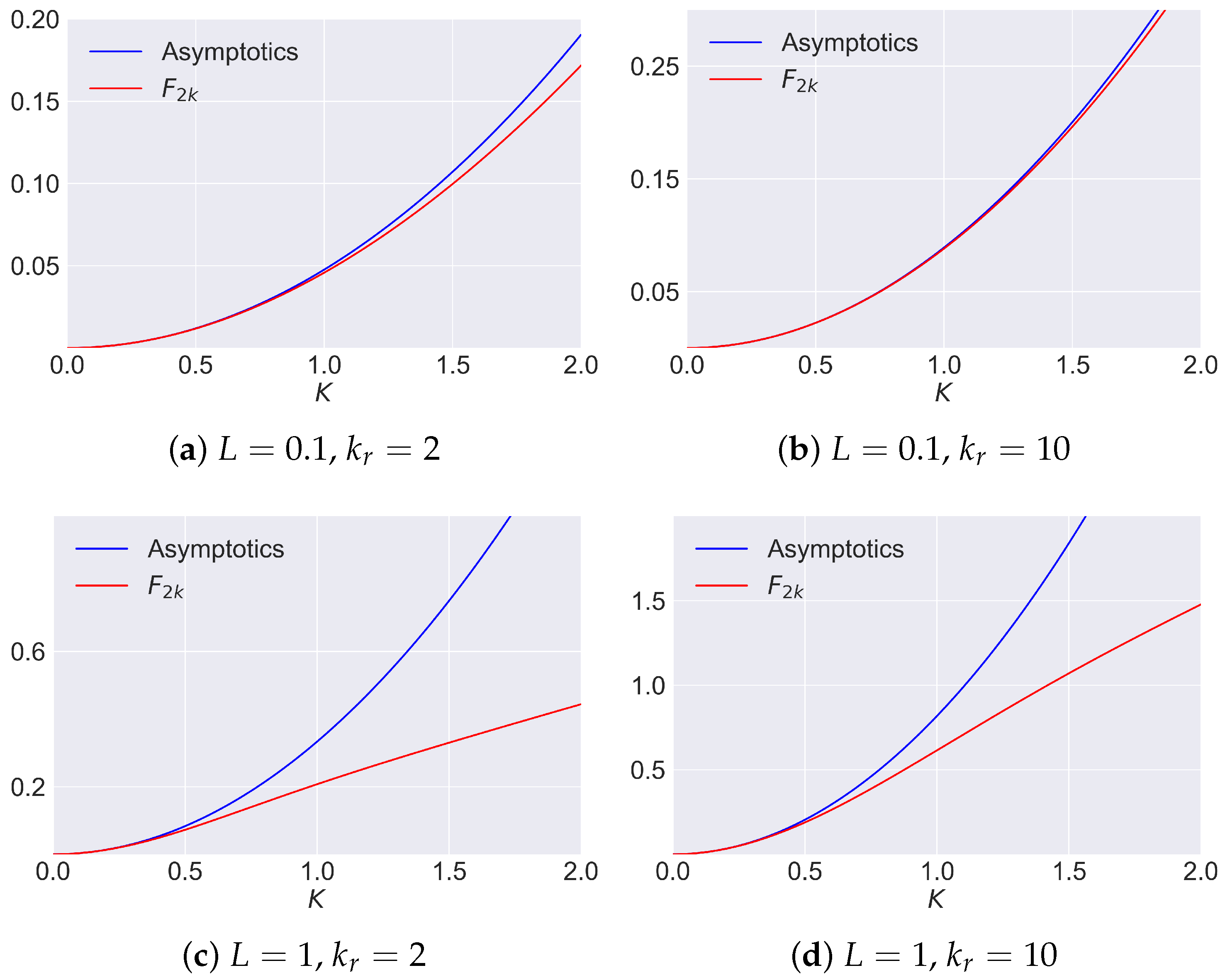
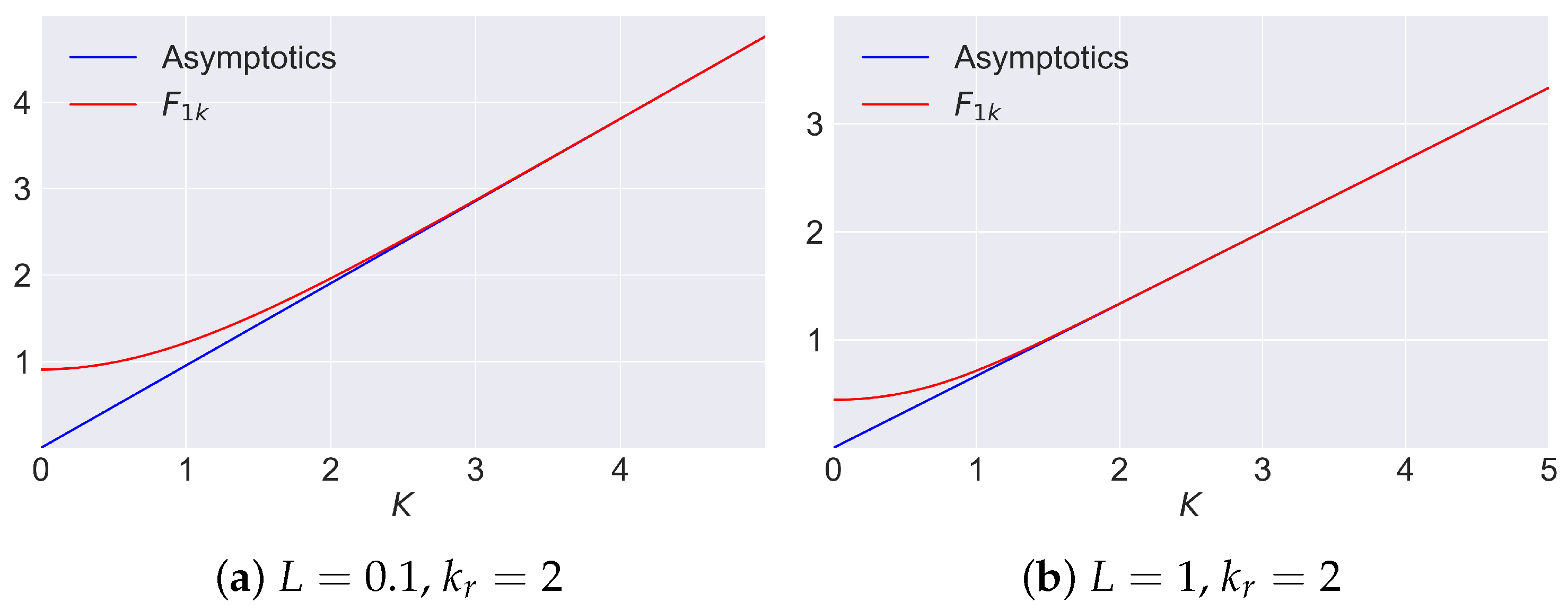
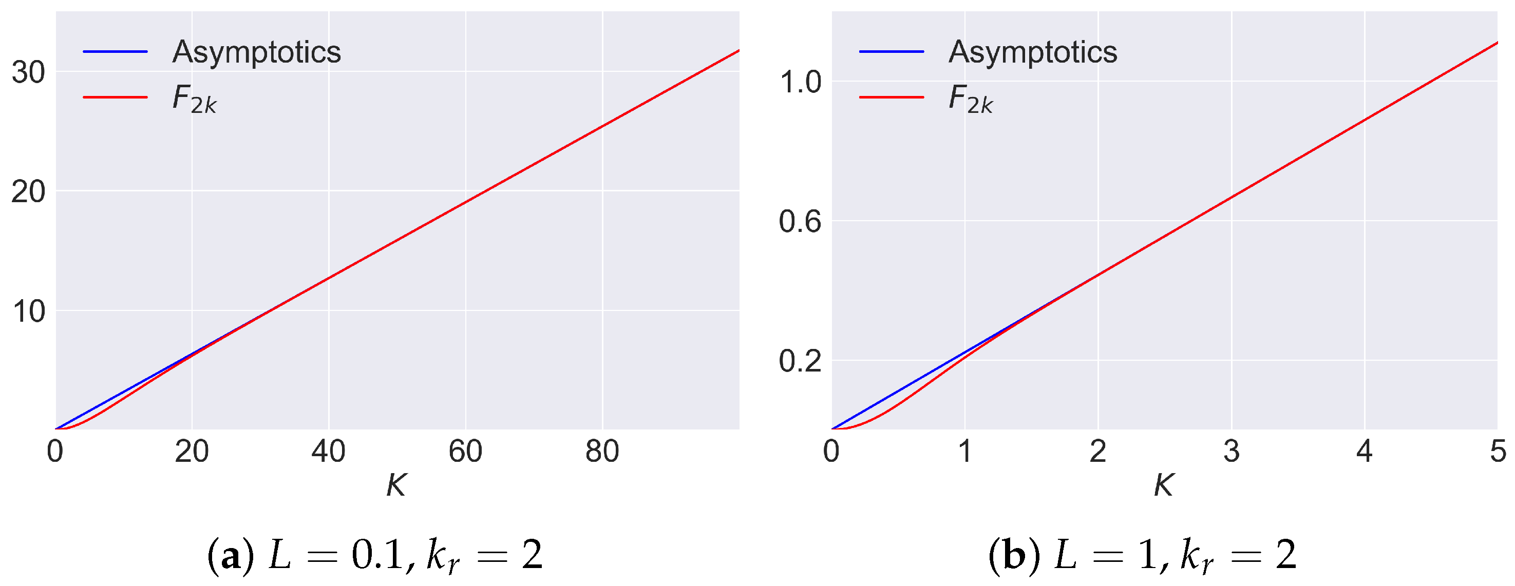
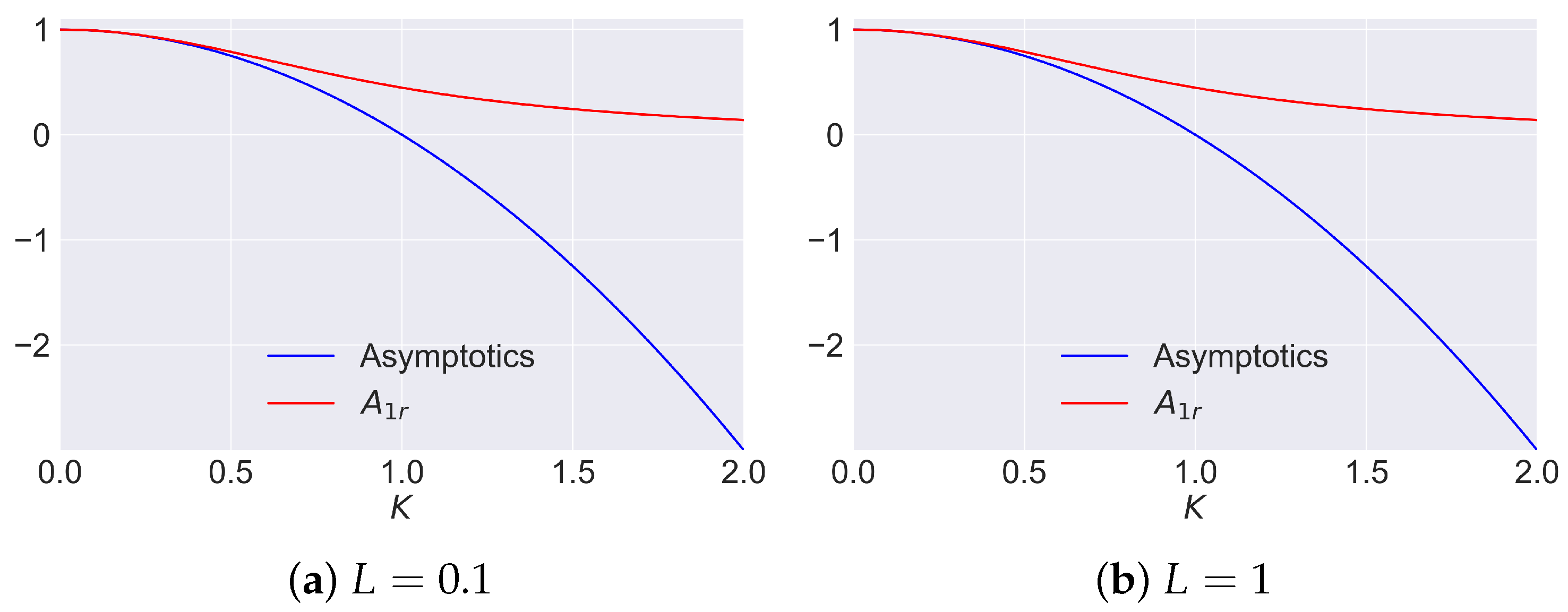
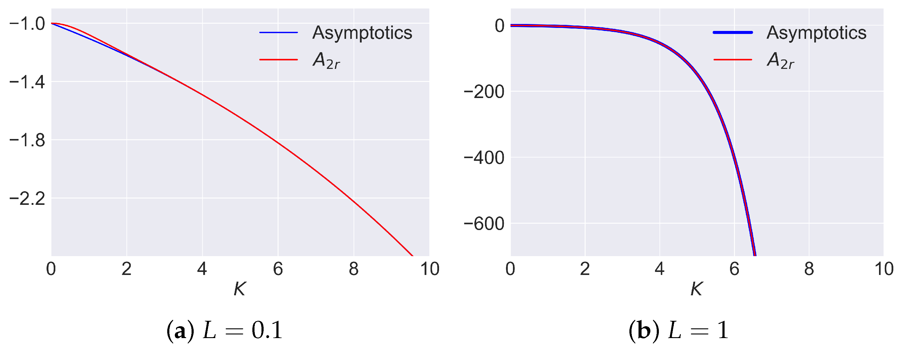
Approximate expressions for
at
and
are obtained in
Appendix A.
Next, we consider the filtration flow without gravity since, as shown in [
7], the presence of gravity does not affect the fundamental features of the instability development in the considered problem. We put
in (
72)–(
78) and obtain:
From the expressions (
66) and (
67), it follows that the ratio of coefficients
is equal to the ratio of perturbation amplitudes at the water–oil and water–gas boundaries. We introduce the variables
at
and
at
. From the system of Equations (
70), we find
where
We consider the case when, at the initial moment, there are perturbations of the gas–water interfaces and water–oil interface in the form of
Under such initial conditions, the solution has the form
where the coefficients
,
,
and
are connected by the relations
From Equations (
89)–(
92), we find
By replacing the relations (
93)–(
96) in the solution of (
87) and (
88), we obtain
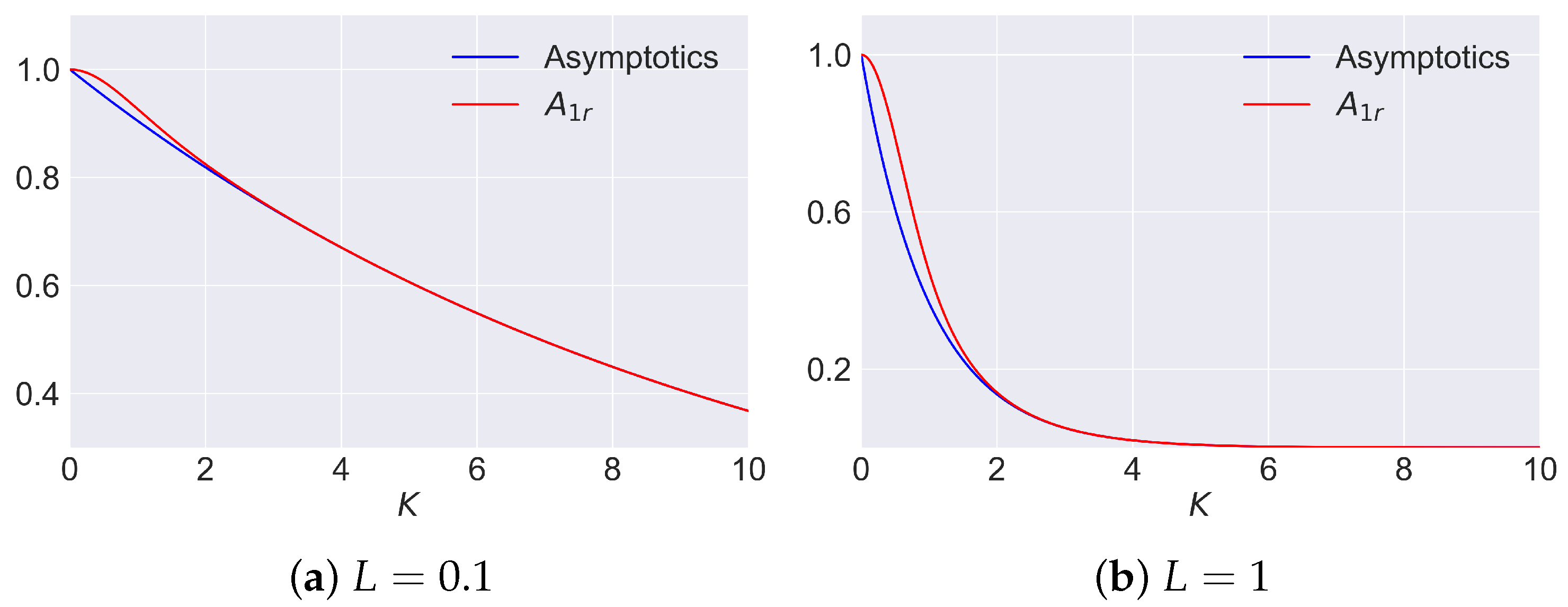
Approximate expressions for
and
at
and
are obtained in
Appendix A.
The linearized equations (
61) and (
62) are found under the assumption that
Then, if the functions
and
are of the form (
66) and (
67), then the following conditions must be true
Because and are perturbation amplitudes, it follows from the above inequalities that a linear analysis is only applicable when the perturbation amplitude of the interface is much smaller than the wavelength of the perturbation.
5. Discussion of Results
The formation of gas or water fingers in the oil-occupied region is associated with the instability of the gas–water or water–oil boundaries. We will consider the evolution of these boundaries in two cases. In the first case, we will assume that perturbations exist only on the gas–water surface at the initial moment. In the second case, we will assume that there are perturbations on both surfaces at the initial moment, and these perturbations have equal amplitudes.
Let us put
then,
and
, where the superscript ∗ denotes the dimensional quantities and
.
According to [
28], oil’s viscosity can vary from 0.0001 Pa·s to 0.8 Pa·s, while the viscosity of water is 0.001 Pa·s. Thus, the value of
varies from 0.1 to 800.
Substituting
,
,
,
and
into (
41), we obtain that
where
is the time for oil to be completely displaced by water from the reservoir if both interfaces remain flat.
To investigate the effect of gas–water surface perturbation growth on the evolution of the water–oil surface, we consider the case when there is a perturbation of the gas–water interface at the initial moment and the water–oil interface is flat, i.e., .
We denote the amplitude of the water–oil surface perturbation as
and the gas–water perturbation as
; then, we obtain from (
97) and (
98) at
:
The amplitude of the water–gas surface perturbation,
, at time
is
where
.
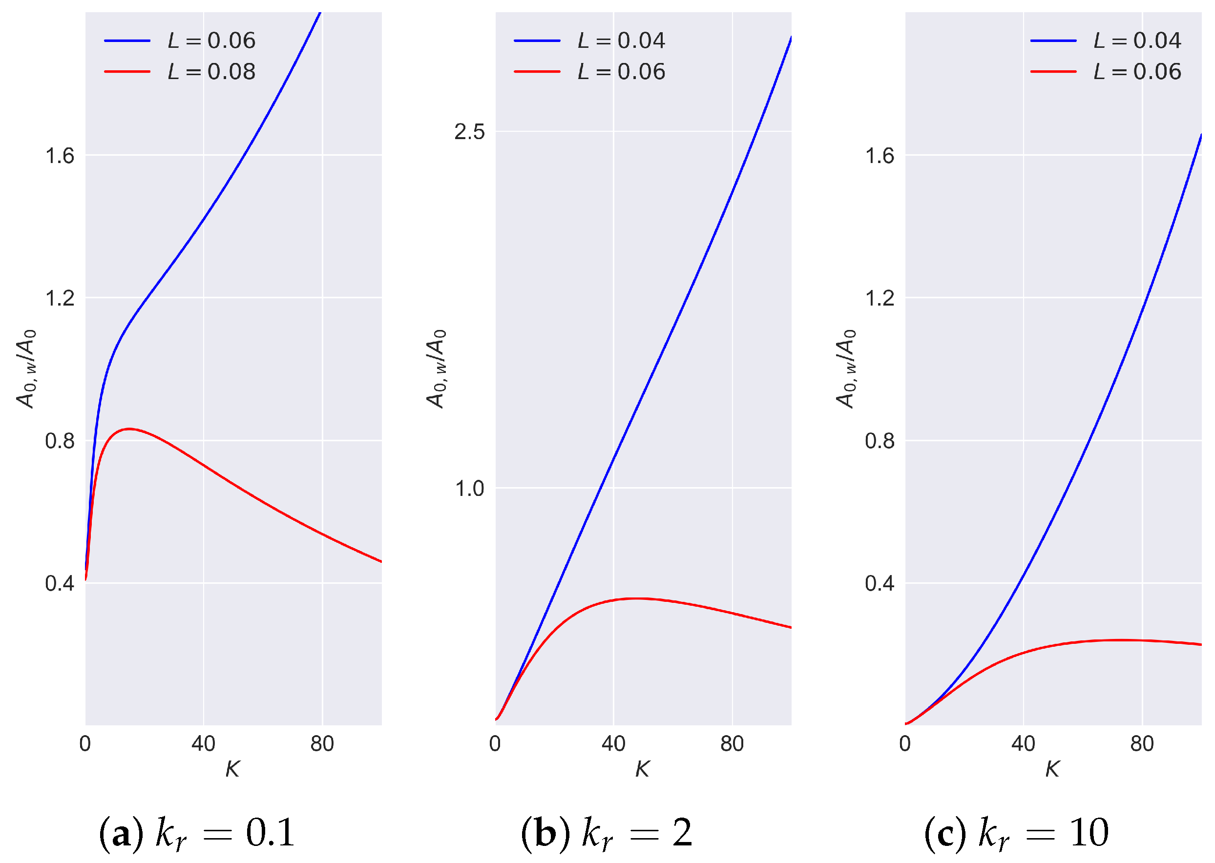
The value of depends on the problem parameters , L, and wave number, K.
In
Figure 2, the dependence of
on
K at different values of
L and
is presented. It is seen that at fixed values of
and
, there exists such a value of
that the value of
grows unlimitedly with increasing
K at
and tends to zero at
. Note that
depends weakly on
since it changes less than twice when
changes by a factor of 100.
To find approximate explicit expression for
at
, we use the approximate expressions for
,
,
and
obtained in
Appendix A. From
at
, and taking into account the relation (
104), we obtain
It follows from the formula (
109) that
does not increase with
if
The inequality (
110) is satisfied at
From (
111), we obtain that if
, then
at
,
at
and
at
. These threshold values of
are consistent with the results presented in
Figure 2.
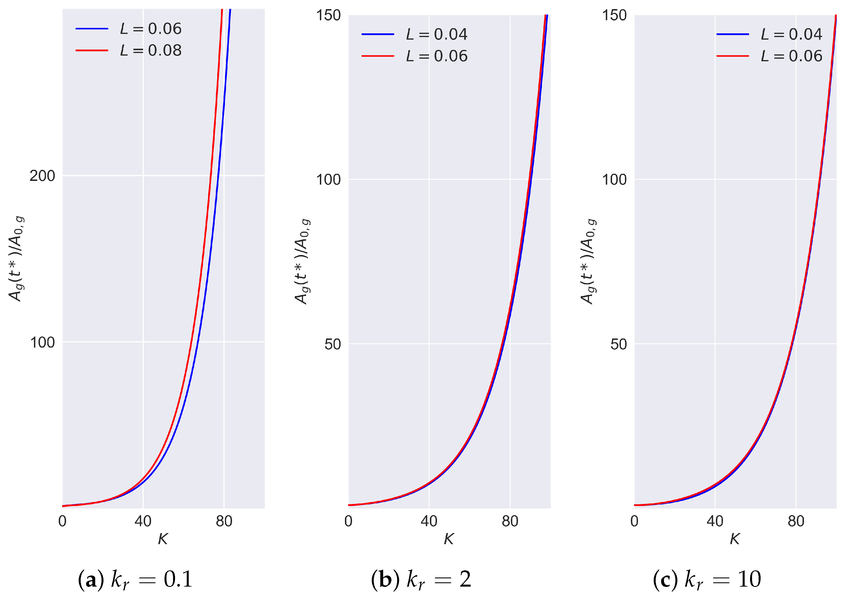
Thus, over time
, the development of short-wave perturbations at the gas–water boundary does not significantly affect the evolution of the water–oil boundary if the thickness of the water layer exceeds
. The velocity perturbations, which are caused by the gas–water boundary instability, decay with a decreasing
z coordinate according to the law
in accordance with (
69). At the initial moments of time, these velocity perturbations are so small at
(at the water–oil surface) that during the time
, the amplitude
increases only up to a value of the order of
. Note that the amplitude of the perturbations of the water–gas surface at time
increases by more than two orders of magnitude for short-wave perturbations with wave number
, as shown in
Figure 3.
For , the viscosity of water is less than that of oil, so the water–oil contact surface is unstable if oil is displaced by water. However, at , instability development occurs at each boundary independently. The growth of perturbations at the gas–water boundary occurs with a characteristic time of , and the growth of perturbations at the water–oil boundary occurs with a characteristic time of . Since , the water–oil boundary perturbations grow slower if the initial perturbation amplitude is comparable to .
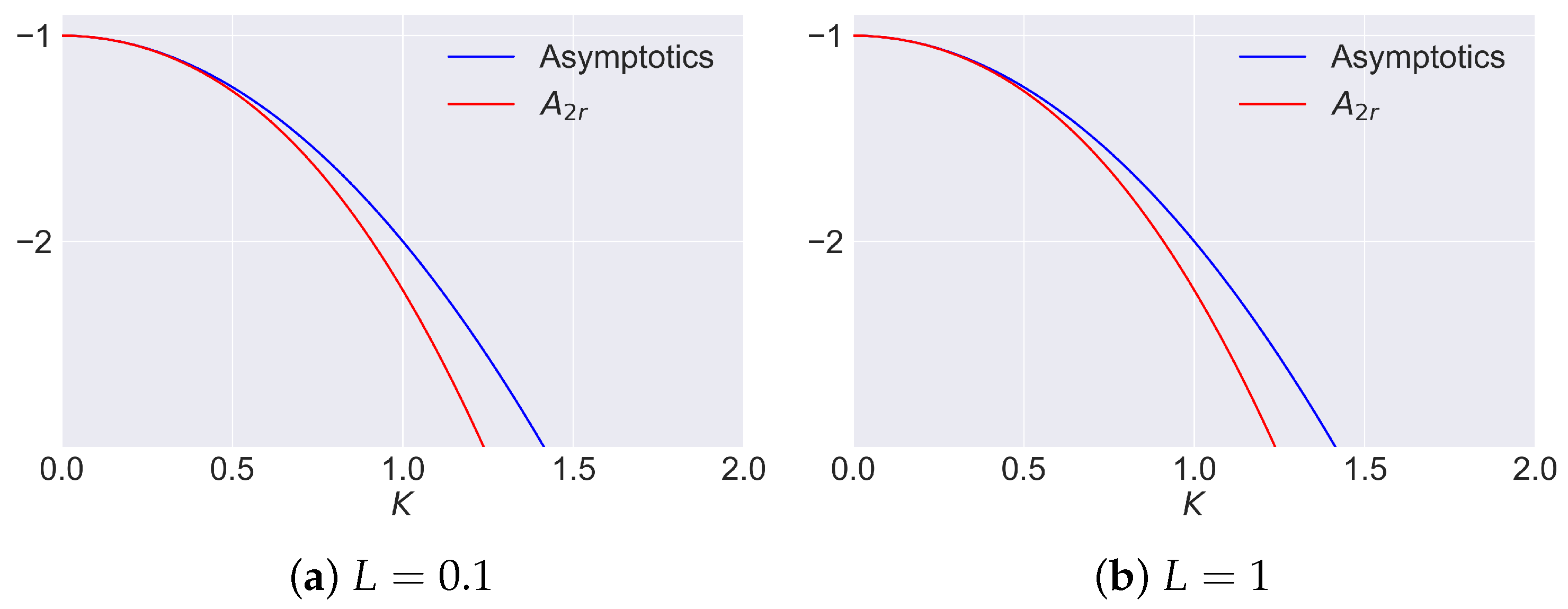
Appendix A shows that the expressions for
and
at
can be written as
From the relations (
112) and (
113), we have
If the perturbation amplitudes are equal at the initial moment, i.e.,
, and the perturbations develop independently, then at
,
Substituting
into the expression (
115), we obtain that
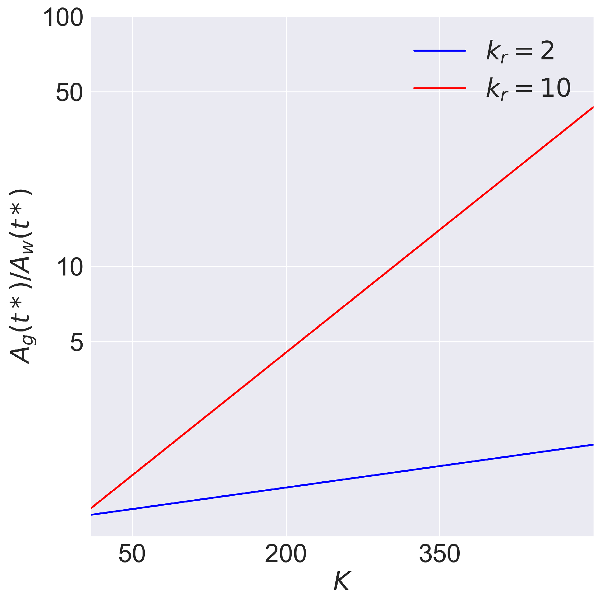
Figure 4 shows the ratio of amplitudes
at time
, calculated from the Formula (
116), for large values of
K.
Figure 4 shows that in the considered case, if the initial perturbation amplitudes of both surfaces are equal, the short-wave perturbations at the water–gas boundary grow faster than at the water–oil boundary.
6. Conclusions
In oil field development, the displacement of oil by gas leads to the formation of gas fingers and areas with residual oil in the reservoir. If there is a layer of water between the gas and oil, gas fingers form in the area occupied by water and form areas with slow-moving water rather than oil. In most cases, oil’s viscosity is more than water’s, so the water–oil boundary is also unstable. The short-wavelength instability of this boundary leads to the formation of water fingers in the region occupied by oil. Using the normal mode method, relations describing the growth of gas–water and water–oil surface perturbations are obtained. These relations describe the evolution of perturbations in the linear approximation, depending on the wavelength of the perturbation and the parameters of the main flow. The study shows that there is a threshold value of water layer thickness, . Suppose the thickness of the water layer is greater than the threshold value. In that case, the development of perturbations at the water–gas boundary has no effect on the development of perturbations for a time comparable to the characteristic time of the oil displacement process. An expression for calculating the threshold value of at given values of oil viscosity, pressure drop and thickness of the low-permeable layer of porous medium containing oil is obtained. It is shown that short-wave perturbations at the water–oil boundary grow much slower than perturbations at the water–gas boundary at the linear stage of perturbation evolution.
It follows from the results that the presence of a water layer between oil and gas significantly reduces the growth of short-wave perturbations (“fingers”) in the oil-occupied region. Thus, the water layer may allow the amount of residual oil to be reduced, which is a big problem for effective production.
The study was performed for small perturbations under the assumption that the wavelength of the perturbation remains much larger than the amplitude. The evolution of perturbations at the nonlinear stage is planned to be investigated in the future using the continuum and network models previously described by the authors in [
9].


