Roadmap of the Multiplier Method for Partial Differential Equations

Abstract

This review paper gives an overview of the method of multipliers for partial differential equations (PDEs). This method has made possible a lot of solutions to PDEs that are of interest in many areas such as applied mathematics, mathematical physics, engineering, etc. Looking at the history of the method and synthesizing the newest developments, we hope to give it the attention that it deserves to help develop the vast amount of work still needed to understand it and make the best use of it. It is also an interesting and a relevant method in itself that could possibly give interesting results in areas of mathematics such as modern algebra, group theory, topology, etc. The paper will be structured in such a manner that the last review known for this method will be presented to understand the theoretical framework of the method and then later work done will be presented. The information of four recent papers further developing the method will be synthesized and presented in such a manner that anyone interested in learning this method will have the most relevant information available and have all details cited for checking.

1. Introduction

When studying mechanical systems, the appearance of PDEs is natural; this opens up the problem of finding methods that make it possible to solve these equations analytically, qualitatively and in the case of many PDEs to find their application to physical problems, finding the conservation laws of PDEs.

There has been a wide list of methods developed recently; here, we review the method of multipliers which has been a fruitful research area giving a lot of advantages over other methods that will be pointed out and commented on throughout the paper.

Like many other similar methods, the method of multipliers tries to find conservation laws through symmetries; this is possible by studying group actions with respect to manifolds.

The study of such group actions was given attention by many mathematicians and physicists such as Felix Klein [1]; thanks to this work in the modern scientific panorama, a lot of huge leaps have been taken in various areas of research and it is still an area in which a lot of open problems are unresolved.

Specifically, the method of multipliers has many virtues compared to many others methods; it is a really impressive tool that can be appreciated by looking back to the early stages of this area (i.e., [2]).

Here, a roadmap of the history and modern developments of the method are going to be synthesized in the most comprehensive manner so they can be used by researchers to achieve more important breakthroughs and also further develop the method that still promises to give a lot.

This method defines symmetries using a geometrical and algebraic perspective as group actions leaving invariant the space of dependent variables and their derivatives to a certain order n and independent variables for a certain PDE system [3].

This is possible thanks to what is known as the infinitesimal generators of a given system, hence introducing Lie groups and Lie algebras that give many of the interesting mathematical aspects of the method of multipliers.

This method was first applied to systems of ODEs [4]; in this paper, an expression was derived that relates symmetries and conservation laws of self-adjoint differential equations, for earlier references on the development of this method check [4,5].

This expression does not need the existence of a Lagrangian and it can obtain conservation laws either from local or non-local symmetries; this was the first step in the generalization of this method to PDEs.

The work carried out in this paper is a consequence of research carried out in [6,7,8].

These papers were the first to state the possibility of there being a relationship between non-local symmetries and what is called potential systems using linearization (Fréchet derivative).

This is the main idea developed for ODEs and PDEs in the method of multipliers, but it is quite a new method that is open to further generalizations.

Some of these generalizations were also made possible by results found in [6,7,8], such as providing a means of knowing the equivalence classes of symmetries for the PDEs or ODEs and also stating the algorithmic nature of this method that made possible computational developments.

From here, a generalization to PDEs followed [9,10,11].

The importance of the method is best understood when compared to other methods like [12,13,14] that do not give the necessary and sufficient conditions to know if an adjoint-symmetry is also a multiplier.

Also, by nature this method is algorithmic as opposed to the other methods mentioned above, which consequently makes the multiplier method less algebraically complicated in many aspects and assures one obtains a result if the conditions imposed are met.

All these developments were synthesized and expanded in the review paper [15]; this is the basis of the historical background we’ll give in this paper.

In this review, a modern form of Noether’s Theorem is proved.

This modern form of Noether’s Theorem formalizes the existing relation between adjoint-symmetries and conservation laws; it provides a way to find conservation laws of not only variational PDEs, but also non-variational PDEs, letting us find either local or non-local symmetries for a given system of PDEs.

Many questions about the method still remain; some have been answered and these new results will be synthesized in the section of this paper titled “Modern Developments”.

One new result that deserves a special mention is the geometrical formulation for adjoint-symmetries that were found to describe one-forms for PDEs and its generalization to systems of evolution equations; it also has spatial constraints in which these adjoint-symmetry one-forms are also invariant up to a functional multiplier for an associated normal one-form for the constraint equations [16].

The other new developments with respect to the method of multipliers can be found in [17,18,19,20].

Following the same order in which they are cited, the first paper gives a generalization of the double reduction method and improvements on the symmetry-invariant condition are made by framing it using multipliers.

The second paper gives an explicit formula to find symmetry recursion operators for PDEs, presenting new results that find relations between integrating factors and non-variational symmetries.

The third paper studies the algebraic structure of the infinitesimal symmetries obtained via the adjoint Fréchet derivative from which the interesting result of having a one-symmetry action that encodes pre-symplectic operators gives rise to a symplectic two-form with Poisson brackets defined for evolution systems.

The section on the historical background will end by giving a revision of high-relevance literature that benefited from this method with the hopes of quantizing the impact the method has had and that it still has.

Some of the results of these papers will be presented here as an example of the use of the method.

In the next section, “Modern Developments”, the newest findings on the method will be presented with some examples of how these results are used in practical cases; finally, in this same section, further steps to develop the method are advised.

The next section, called “Comparison”, will give a direct comparison of this method with similar ones; we’ll give the best explanation of the weaknesses and strengths of this method compared to other method present in the literature.

This paper is divided into four parts. The first part, named “Historical background”, will be dedicated to presenting the method of multipliers as it was presented in the old review [21] and the contributions made possible until that point.

The second part, named “Recent Contributions”, will be dedicated to reviewing the new developments of the method since the old review and the contributions made possible by these developments; further steps with respect to the method are also discussed.

In the third section, “Comparison”, some parallel methods developed alongside the method of multipliers will be explained and we’ll discuss the strengths and weaknesses of the method compared to others.

Finally, a conclusion will be given to wrap up this review.

To end the introduction, a graphical representation of the flow of this review is added for easier and more comprehensive reading of the results presented.

2. Historical Background

The starting point, as said earlier, is the most recent review [21]; we use this review to explain the method in the state it was in at that point and in the end some relevant papers will be commented on and some examples developed.

The examples developed and the general structure of this section can be checked in in Figure 1.

2.1. Theory

The method of multipliers helps to find conserved integrals and local continuity equations of PDEs. From these objects, we can find conserved quantities, constants of motion of the system and a lot of extra information that is useful in the study of PDEs.

As an example, in three dimensions, the local continuity equations have the next form for their total divergence

$$D_{t}T+Div\overrightarrow{X}=0.$$

(1)

This expression yields the next physical conservation law

$$\frac{d}{dt}{\int }_{\Omega }TdV=-{\oint }_{\delta \Sigma }\overrightarrow{X}·\overrightarrow{\nu }dA$$

(2)

where $\Omega$ is the spatial domain and $\overrightarrow{\nu }$ is the outward unit normal of the domain boundary. This type of expression can be solved using Noether’s Theorem [22] as stated in the review paper. The importance of the method of multipliers is that it can obtain equations of continuity of PDEs that do not posses a variational principle using a modern form of Noether’s Theorem.

These so-called multipliers can be thought of as integrator factors for PDEs; these integrator factors enable us to obtain a linear system of determining equations for the PDE system with no restrictions on the system.

This method also assures we obtain all the conserved integrals from multipliers for systems of Cauchy–Kovalevskaya form.

The history of Noether’s Theorem and the method of multipliers can be found in [23].

This modern form of Noether’s Theorem can be traced back to [9,10,11,24]; this generalization of Noether’s Theorem arises from the system of determining equations that, for the method of multipliers, is an augmented adjoint version of the typical determining equations for infinitesimal symmetries.

By finding this multipliers, the conservation laws determined by the system are found with the use of various known integration methods [14].

The advantage of this method apart from the possibility of working without PDE systems with a variational principle is the algorithmic nature of it; there is no need of anstazes for solving the systems as in other methods such as the ones presented in [25,26,27,28].

To state the important results of the method of multipliers until this point, the following notation is used. Let t, $x=(x^1,\dots ,x^n)$ be independent variables, $n\ge 1$, and let $u=(u^1,\dots ,u^n)$ be dependent variables. Partial derivatives of u with respect to t,x will be written as $\partial u=(u_t,u_{x^1},\dots ,u_{x^n})$ and the kth-order partial derivatives are denoted ${\partial }^{k}u$, $k\ge 2$. The coordinate space $J=(t,x,u,\partial u,{\partial }^{2}u,\dots )$ is called the jet space. Partial derivatives with respect to these variables are given by $\partial /\partial t,\partial /\partial x={(\partial /\partial x^1,\dots ,\partial /\partial x^n)}^t,\partial /\partial u={(\partial /\partial u^1,\dots ,\partial /\partial u^m)}^t$; the superscript t denotes the transpose. Total derivatives are written as $D=(D_t,D_{X^1},\dots ,D_{x^n})$. In particular, $Du=\partial u$, $D\partial u={\partial }^{2}u$. $D^k$ denotes all of the kth-order derivatives with respect to t,x. Divergences are expressed as $Div=D_x·$.

A system of Nth order of $M\ge 1$ PDEs

$$G=(G^1(t,x,u,\partial u,\dots ,{\partial }^{N}u),\dots ,G^M(t,x,u,\partial u,\dots ,{\partial }^{N}u))$$

(3)

will have a space of locally smooth solutions $u(t,x)$ denoted by $\mathcal{E}$. This space is embedded in J since $u(t,x)\in \mathcal{E}$ determines $(t,x,u(t,x),\partial u(t,x),{\partial }^{2}u(t,x),\dots )\in J$.

A local conservation law of a given PDE system (3) is a local continuity equation [17]

$$(D_{t}T+D_x·X){|}_{\mathcal{E}}=0$$

(4)

where T is the conserved density and X is the spatial flux. The pair

$$(T,X)=\Omega$$

(5)

is known as a conserved current.

When this conservation law (4) is integrated, the following expression is obtained.

$$\frac{d}{dt}{\int }_{\Omega }T{{|}_{\mathcal{E}}dV=-{\oint }_{\partial \Omega }X|}_{\mathcal{E}}·\nu dA$$

(6)

and the change of rate of the quantity

$$\mathcal{C}\left[u\right]={\int }_{\Gamma }{T|}_{\mathcal{E}}dV$$

(7)

where $\Omega$ is any spatial domain $\Omega \subseteq {\mathbb{R}}^n$, $\partial \Omega$ is the boundary of the spatial domain and $\nu$ denotes the outward pointing unit normal vector.

The quantity (7) is known as a conserved integral and Equation (6) is called a global conservation law.

An infinitesimal symmetry of a system (3) is given by a generator of the form

$$\mathbf{X}=\tau \partial /\partial t+\xi \partial /\partial x+\eta \partial /\partial u$$

(8)

with the condition that the prolongation leaves invariant the PDE system [2]

$${pr\mathbf{X}\left(G\right)|}_{\mathcal{E}}=0$$

(9)

The functions in (8) are known as the characteristic functions for the symmetry generator; by exponentiating this infinitesimal symmetry, we can obtain a one-parameter group of transformations $exp\left(ϵpr\mathbf{X}\right)$; the infinitesimal transformation is then given by

$$\begin{array}{c}u(t,x)\to u(t,x)+ϵ\left(\eta (t,x,u,\partial u,\dots ,{\partial }^{r}u)\right)-u_t(t,x)\tau (t,x,u,\partial u,\dots ,{\partial }^{r}u)\hfill \\ \hspace{1em}\hspace{1em}\hspace{1em}\hspace{1em}\hspace{1em}\hspace{1em}\hspace{1em}\hspace{1em}\hspace{1em}\hspace{1em}\hspace{1em}\hspace{1em}\hspace{1em}\hspace{1em}\hspace{1em}-u_x(t,x)·\xi (t,x,u,\partial u,\dots ,{\partial }^{r}u)+O\left({ϵ}^2\right).\hfill \end{array}$$

(10)

Next, we define a point symmetry as a symmetry transformation group on $(t,x,u)$, having a generator with a characteristic form in the same form as (8); this corresponds to an infinitesimal point transformation [17]

$$\begin{array}{cc}\hfill t& \to t+ϵ\tau (t,x,u)+O\left({ϵ}^2\right)\hfill \end{array}$$

(11)

$$\begin{array}{cc}\hfill x& \to x+ϵ\xi (t,x,u)+O\left({ϵ}^2\right)\hfill \end{array}$$

(12)

$$\begin{array}{cc}\hfill u& \to u+ϵ\nu (x,t,u)+O\left({ϵ}^2\right).\hfill \end{array}$$

(13)

Next, we define a contact symmetry as a symmetry transformation group on $t,x,u,u_t,u_x$ that also satisfies the contact relations $u_t={\partial }_{t}u$, $u_x={\partial }_{x}u$. The set of all the point symmetries and contact symmetries of a PDE system is the group of Lie symmetries.

The group of Lie symmetries is all the point symmetries and contact symmetries for the given PDE system.

As the first step to finding if a certain current (5) is a conserved one for a given PDE system and to know if a generator (8) is an infinitesimal symmetry for a given PDE system, it is necessary to give coordinates to the solution space $\mathcal{E}$ of the system in the jet space J [17].

The first step to coordinate is to indicate with indices the different dependent and independent variables that describe the system $x^i$, $i=1,\dots ,n$ and $u^{\alpha }$, $\alpha =1,\dots ,m$; next, suppose each PDE $G^a=0$, $a=1,\dots ,M$ in the given system can be rewritten in a solved form in the following way

$$G^a={\partial }_{la}{u}^{{\alpha }_a}-g^a$$

(14)

for a derivative of a dependent variable $u^{{\alpha }_a}$ with the restriction that the other terms present in the system present neither this derivative nor the differential consequences of this dependent variable.

$${\partial }_{la}{u}^{{\alpha }_a}-g^a\ne {\partial }^k{\partial }_{lb}{u}^{{\alpha }_b}-g^a,a,b=1,\dots ,Mk\ge 1$$

(15)

$$\frac{\partial g^a}{\partial \left({\partial }^k{\partial }_{l_b}{u}^{a_b}\right)}=0,a,b=1,\dots ,M,k\ge 0.$$

(16)

These derivatives are the so-called leading derivatives of the system. A closed PDE system (3) that admits these solved forms (14)–(16) is called regular [17].

For the development of the method, there are some tools that we require from variational calculus; here, we only present the main results needed, all derivations and extra information can be found in [17].

The first important tool borrowed from variational calculus is the Fréchet derivative; this derivative is defined as

$${\delta }_{\nu }f=\frac{\partial }{\partial ϵ}f(t,x,u+ϵ\nu ,\dots ,{\partial }^k(u+ϵ\nu )){|}_{ϵ=0}=\nu \frac{\partial f}{\partial u}+\dots +D^k\nu ·\frac{\partial f}{\partial \left({\partial }^{k}u\right)}$$

(17)

This derivative is the linearization of the function; it is interpreted as a local directional derivative in jet space J; this linearization corresponds to an action $\widehat{\mathbf{X}}=v{\partial }_u$ in characteristic form, $\widehat{\mathbf{X}}={\delta }_{v}f$.

The Fréchet adjoint derivative is defined as follows

$$w{\delta }_{\nu }f-\nu {\delta }_w^{\ast }=D·\Psi (\nu ,w;f)$$

(18)

which defines a linear differential operator that acts on w. The associated current $\Psi (v,w;f)=({\Psi }^t,{\Psi }^x)$ is defined as

$$\begin{array}{c}\Psi (v,w;f)=vw\frac{\partial f}{\partial (\partial u)}+\left(Dv\right)·\left(w\frac{\partial f}{\partial \left({\partial }^{2}u\right)}\right)-vd·\left(w\frac{\partial f}{\partial \left({\partial }^{2}u\right)}\right)+\hfill \\ \hspace{1em}\hspace{1em}\hspace{1em}\hspace{1em}\hspace{1em}\hspace{1em}\hspace{1em}\hspace{1em}\hspace{1em}\hspace{1em}\hspace{1em}\hspace{1em}\hspace{1em}\hspace{1em}\hspace{1em}\dots +\sum _{l=1}^k\left(D^{k-l}v\right)·\left({(-D)}^{l-1}·\left(w\frac{\partial f}{\partial \left({\partial }^{k}u\right)}\right)\right)\hfill \end{array}$$

(19)

The function f can be defined as follows: when $u=0$ is non-singular, then a homotopy curve $u_{\left(\lambda \right)}(t,x)$ can be defined to be a homogeneous line and therefore it gives the following expression

$${f=f|}_{u=0}+{\int }_0^1\left({\partial }_{\nu }f\right){|}_{u=u_{\left(\lambda \right)}}\frac{d\lambda }{\lambda },u_{\left(\lambda \right)}=\lambda u$$

(20)

The Euler operator is written in terms of the Fréchet derivative as follows

$${\partial }_{\nu }f=\nu E_u\left(f\right)+D·{\mathsf{{\rm Y}}}_f\left(\nu \right)$$

(21)

which gives

$$E_u\left(f\right)=\frac{\partial f}{\partial u}-D·\left(\frac{\partial f}{\partial (\partial u)}\right)+\dots +{(-D)}^k·\left(\frac{\partial f}{\partial \left({\partial }^{k}u\right)}\right).$$

(22)

where

$${\mathsf{{\rm Y}}}_f\left(v\right)=\Psi (v,1;f)=\sum _{l=0}^{k-1}(D^{l}v·E_{{\partial }^{l+1}u}\left(f\right)$$

(23)

This expression lets us state the next four useful lemmas stated in [21].

Lemma 1. 

$$f={\int }_0^1{\partial }_{\lambda }{u}_{\left(\lambda \right)}{E}_u{\left(f\right)|}_{u=u_{\left(\lambda \right)}}d\lambda +D·F$$

(24)

is an identity, where

$$F={\int }_0^1{\mathsf{{\rm Y}}}_f\left({\partial }_{\lambda }{u}_{\left(\lambda \right)}\right){|}_{u=u_{\left(\lambda \right)}}d\lambda +F_0$$

(25)

with $F_0=(F_0^t(t,x),F_0^x(t,x))$ being any current such that $D·F_0{=f|}_{u=u_0}$

A useful relation is

$${\mathsf{{\rm Y}}}_f\left(\nu \right)=\nu E_u^{\left(1\right)}\left(f\right)+D·\left(\nu E_u^{\left(2\right)}\left(f\right)\right)+\dots +D^{k-1}·\left(\nu E_u^{\left(k\right)}\left(f\right)\right)$$

(26)

which is obtained via repeated integration of (23), where

$$\begin{array}{c}\hfill E_u^{\left(l\right)}\left(f\right)=\frac{\partial f}{\partial \left({\partial }^{l}u\right)}-\left(\genfrac{}{}{0pt}{}{l+1}{l}\right)D·\left(\frac{\partial }{\partial \left({\partial }^{l+1}u\right)}\right)+\dots +\left(\genfrac{}{}{0pt}{}{k}{l}\right){(-D)}^{k-l}·\left(\frac{\partial f}{\partial \left({\partial }^{k}u\right)}\right),l=1,\dots ,k\end{array}$$

(27)

defines the higher Euler operators.

From Equations (21)–(23) we can obtain an alternative formula for the Fréchet derivative.

$${\partial }_{v}f=v{E}_u\left(f\right)+D·\left(v{E}_u^{\left(1\right)}\left(f\right)\right)+\cdots +D^k·\left(v{E}_u^{\left(k\right)}\left(f\right)\right)$$

with the following adjoint derivative

$${\delta }_w^{\ast }f=w{E}_u\left(f\right)-\left(Dw\right)·E_u^{\left(1\right)}\left(f\right)+\cdots +{(-D)}^{k}w·E_u^{\left(k\right)}\left(f\right)$$

Coordinate formulas for this Fréchet derivative and its adjoint counterpart, as well as the associated divergence, are found in [15].

The next lemma gives important properties of the Euler operators (22) and (26) [21].

Lemma 2. 

(i) $E_u\left(fg\right)={\delta }_g^{\ast }f+{\delta }_f^{\ast }g$ is a product rule. (ii) $E_u\left(f\right)=0$ is valid if and only if $f=D·F$ for some differential current function $F=(F^t,F^x)$. (iii) $E_u^{\left(1\right)}(D·F)=E_u(F^t,F^x)=(E_u\left(F^t\right),E_u\left(F^x\right))y{E}_u^{l+1}(D·F)=(E_u^{\left(l\right)},E_u^{\left(l\right)})☉(F^t,F^x),l\ge 1$ are descent rules, where ☉ is the symmetric tensor product.

The next lemma relates null divergences and total curls in jet space; a null divergence is defined as a total divergence $D·\Phi =0$ that vanishes identically in jet space, where $\Phi =({\Phi }^t,{\Phi }^x)$ is defined as a differential current function and the relation between null divergences and total curls in jet space is as follows [21].

Lemma 3. 

If a differential current function $\Phi =({\Phi }^t(t,x,u,\partial u,\dots ,{\partial }^{k}u),{\partial }^x(t,x,u,\partial u,\dots ,{\partial }^{k}u))$ has a null divergence

$$D·\Psi =D_t{\Psi }^t+D_x·{\Psi }^x=0\mathrm{in}J,$$

(28)

then it is equal to a total curl

$$\Phi =D·\Psi =(D_x·\Theta ,-D_t\Theta +D_x·\Gamma )\mathrm{in}J$$

with

$$\left(\begin{array}{cc}0& \Theta \\ -\Theta & 0\end{array}\right)$$

being valid for a given vector function $\Theta (t,x,u,\partial u,\dots ,{\partial }^{k-1}u)$ and some differential anti-symmetric tensor function $\Gamma (t,x,u,\partial u,\dots ,{\partial }^{k-1}u)$, where both can then be expressed in terms of ${\Phi }^t,{\Phi }^x$.

Lemma 4. 

If a differential function $f(t,x,u,\partial u,\dots ,{\partial }^{k}u)$ goes to zero on the solution space $\mathcal{E}$ for some regular system of PDEs, then

$$f=R_f\left(G\right)$$

(29)

holds identically, where

$$R_f=R_f^{\left(0\right)}+R_f^{\left(1\right)}·D+\cdots +R_f^{(k-N)}·D^{k-N}$$

(30)

is a linear differential operator that depends on f with coefficients $\mathcal{E}$$R_f^{\left(0\right)},R_f^{\left(1\right)},\dots ,R_f^{(k-N)}$. The operator $R_f{|}_{\mathcal{E}}$ is canonically determined by f if there are no differentiable identities. If the PDE system satisfies a differential identity

$$\mathcal{D}\left(G\right)={\mathcal{D}}_1{G}^1+\cdots +{\mathcal{D}}_M{G}^M=0$$

(31)

with ${\mathcal{D}}_1+\dots ,{\mathcal{D}}_M$ being linear differential operators, with non-singular differential functions on $\mathcal{E}$, then the operator $R_f{|}_{\mathcal{E}}$ is a canonically determined modulo $\mathcal{X}\mathcal{D}$, with $\mathcal{X}$ being an arbitrary differential function.

Joining these elements of variational calculus and infinitesimal symmetries like (8) of a system of PDEs (3), we can obtain a symmetry generator that acts on the solution space of the PDE system in jet space as

$$\widehat{\mathbf{X}}=\mathbf{X}-{\mathbf{X}}_{triv}=P\frac{\partial }{\partial u},P=\eta -u_t\tau -u_x·\xi$$

(32)

where ${\mathbf{X}}_{triv}$ is defined in [17]. This is the generator that gives the characteristic form for the infinitesimal symmetry. Now, we can rewrite the symmetry invariance (9) as

$$pr\widehat{\mathbf{X}}{\left(G\right)|}_{\mathcal{E}}=0$$

(33)

The Fréchet derivative is equivalent to the action of the prolongation, so we can rewrite again Equation (33) as

$$\left({\delta }_{P}G\right){|}_{\mathcal{E}}=0$$

(34)

Now, with a conservation law (4) of a regular PDE system (3), we can use Equations (29) and (30) to show that a conservation law can be written as [21].

$$D_{t}T+D_x·X=R_{\Phi }\left(G\right)=R_{\Phi }^{\left(0\right)}{G}^t+R_{\Phi }^{\left(1\right)}·D{G}^t+\cdots +R_{\Phi }^{(r+1-N)}·D^{r+1-N}{G}^t$$

(35)

From this expression, we arrive at

$$D_t\tilde{T}+D_x·\tilde{X}=GQ$$

(36)

with

$$\begin{array}{c}(\tilde{T},\tilde{X})=(T,X)+R_{\Psi }^{\left(1\right)}{G}^t+R_{\Phi }^{\left(2\right)}·D{G}^T-(D·R_{\Phi }^{\left(2\right)})G^t+\cdots +\hfill \\ \hspace{1em}\hspace{1em}\hspace{1em}\hspace{1em}\hspace{1em}\hspace{1em}\hspace{1em}\hspace{1em}\hspace{1em}\hspace{1em}\hspace{1em}\hspace{1em}\hspace{1em}\hspace{1em}\hspace{1em}\hspace{1em}\hspace{1em}\sum _{l=0}^{r-N}({(-D)}^l·R_{\Psi }^{(r+1-N)})·D^{r-N-l}{G}^t\hfill \end{array}$$

(37)

and

$$Q^t=(Q_1,\dots ,Q_M)=R_{\Psi }^{\left(0\right)}-D·R_{\Psi }^{\left(1\right)}+\cdots +{(-D)}^{r+1-N}·R_{\Psi }^{(r+1-N)}$$

(38)

In the space of solutions, we obtain that

$$(D_t\tilde{T}+D_x·\tilde{X}){|}_{\mathcal{E}}=0$$

(39)

Equation (36) is the characteristic equation rewritten using the tools of variational calculus and Equation (38) is what we define as the multipliers of the system.

The functions

$$Q={(Q_1(t,x,u,\partial u,{\partial }^{2}u,\dots ,{\partial }^{r}u),\dots ,Q_M(t,x,u,\partial u,{\partial }^{2}u,\dots ,{\partial }^{r}u))}^t$$

(40)

are a multiplier if and only if each of them are non-singular on the solution space of the PDE and the summed products with the expressions $G=(G^1,\dots ,G^M)$ of these functions for the PDEs have the form of a total space-time divergence [17].

From Lemma 2, an expression for finding all multipliers for a given PDE system (3) can be stated as follows

$$0=E_u\left(GQ\right)={\delta }_Q^{\ast }G+{\delta }_G^{\ast }Q$$

(41)

This expression holds identically in jet space and is necessary and sufficient for Q to be a multiplier. Using Lemma 1, a corresponding conserved current from each multiplier Q can be obtained from $f=QG$ yielding

$$\tilde{\Psi }={\int }_0^1{\mathsf{{\rm Y}}}_{GQ}\left({\partial }_{\lambda }{u}_{\left(\lambda \right)}\right){|}_{u=u_{\left(\lambda \right)}}d\lambda$$

(42)

The following explicit formula for a conserved current is obtained and reads as follows [21].

Lemma 5. 

For a system of PDEs (3), each multiplier (38) describes a conserved current (36) that is given by a homotopy integral

$$\tilde{T}={\int }_0^1\left(\sum _{l=0}^{k-1}{\partial }_{\lambda }{\partial }_{u_{\left(\lambda \right)}}^l·\left(E_{{\partial }^t{\partial }_{tu}}\left(GQ\right)\right){|}_{u=u_{\left(\lambda \right)}}\right)d\lambda +D_x·\Theta ,$$

(43)

$$\tilde{X}={\int }_0^1\left(\sum _{l=0}^{k-1}{\partial }_{\lambda }{\partial }_{u_{\left(\lambda \right)}}^l·\left(E_{{\partial }^t{\partial }_{tu}}\left(GQ\right)\right){|}_{u=u_{\left(\lambda \right)}}\right)d\lambda -D_t·\Theta +D_x·\Gamma ,$$

(44)

along a homotopy curve $u_{\left(\lambda \right)}(t,x)$, with $u_{\left(1\right)}=u$ y $u_{\left(0\right)}=u_0$ such that ${\left(GQ\right)|}_{u=u_0}$ is non-singular. Here, $k=max(r,N)$

These results make it possible to write the characteristic equation using the adjoint Fréchet derivative in the solution space as

$$\left({\delta }_Q^{\ast }G\right){|}_{\mathcal{E}}=0$$

(45)

The solutions $\mathit{Q}(t,x,u,\partial u,\dots ,{\partial }^{2}u)$ for this determining equation are called adjoint-symmetries [4,6,7,8,9].

Q also satisfies the identity

$${\delta }_Q^{\ast }G={\delta }_{Q^t}^{\ast }{G}^t=R_{Q^t}\left(G^t\right)$$

(46)

found in Lemma 4, where

$$R_{Q^t}=R_{Q^T}^{\left(0\right)},R_{Q^T}^{\left(1\right)}·D+R_{Q^T}^{\left(2\right)}·D^2+\cdots +R_{Q^T}^{\left(r\right)}·D^r$$

(47)

Using these results, the determining Equation (41) can be rewritten as

$$0=R_{Q^T}\left(G^t\right)+{\delta }_G^{\ast }Q$$

(48)

When the PDEs are expressed (deleted) in solved form in terms of a set of leading derivatives, we obtain the following linear system of equations

$$0=R_{Q^T}^{\left(k\right)}+{(-1)}^k{E}_u^{\left(k\right)}\left(Q^t\right),k=0,1,\dots ,r$$

(49)

With this, the next theorem can be stated [21].

Theorem 1. 

The determining Equation (45) for multipliers of conservation laws for any regular system of PDEs (3) is equivalent to the system of linear Equations (45) and (49). In particular, the multipliers are adjoint-symmetries (45) that satisfy Helmholtz-type conditions (49); these are sufficient and necessary for an adjoint-symmetry $Q(t,x,u,\partial u,\dots ,{\partial }^{r}u)$ to have a variational form (21) derived from a conserved current $\Phi =(T,X^i)$.

This theorem is a generalization of the modern form of Noether’s Theorem where symmetries are replaced by adjoint-symmetries to find conservation laws for non-variational PDEs, where the older method was built to find conservation laws of variational PDEs.

The main advantages of this method up this point are the ease it provides in finding all the given conservation laws of systems of PDEs compared to other methods; the main thing that makes this possible is the algorithmic nature of the method.

This also provides the advantage of making possible the use of computational tools to reduce the manual work necessary for finding conservation laws; work has been done and it can be revised in [29,30,31,32] for extra details on the computational implementation of the method.

Another great advantage provided by this method is the size of the system of equations that describe the system; this system of equations is over-determined and makes the process of solving PDEs either by hand or computationally faster and easier compared to other methods.

Contributions

This review paper has a great amount of useful information for studying a wide variety of partial differential equations; since the year it was published until now, at least 149 research papers have used its results; this number comes without taking into account the other citations of the previous papers published describing the same method.

This is a remarkable amount of citations for a topic of this kind and it shows how much impact it had and can continue to have if it gets to more fellow scientists.

One of the most important characteristics of this research is that it can be applied to almost any topic of science; this is a method for general PDEs and they appear naturally in all fields; to make this statement even more clear, a quick overview of different papers citing this one is given and some examples are presented.

Two areas of science that have taken the most advantage of this method are applied mathematics and physics; these two areas can sometimes become very similar to one another, but almost all of the phenomena they study arises from PDEs.

For example, the study of solitons, which concerns both applied mathematics and physics, has seen great developments thanks to the method of multipliers; for example, equations such as the BKP–Boussinesq equation [33] are known to have soliton solutions [34] and their conservation laws were found thanks to the multiplier method in an effort to know more about this recently introduced equation.

More research done in this area can be found in [35] where all low-order conservation laws for this equation are found.

In other papers such as [36], conservation laws, symmetries and line soliton solutions are studied for the Boussinesq and generalized KP equation in two dimensions with nonlinearities.

In [37], the symmetry solutions and conservation laws of a $(3+1)$-dimensional generalized KP–Boussinesq for fluid mechanics is studied; these types of equations are common in the modelling of waves in shallow waters, so the development of the multiplier method has proven useful for applied mathematicians and engineers.

Another equation that has been studied widely using the method of multipliers is the KdV equation; for example, in [38], closed solutions and conserved vectors of the $(3+1)$-dimensional negative-order KdV equations were found.

In [39], Lie symmetries, conservation laws and exact solutions for a generalized quasilinear KdV equation with degenerate dispersion were found.

Lastly, in [40], conservation laws for a generalized seventh-order KdV equation where found.

The KdV equation has gained all this attention because of the wide uses it has in many fields; in [41], some of them are listed and explained.

To name some of the applications of the KdV equation, this equation is used for modelling of surface gravity waves, internal solitons in the ocean, voidage slugs in fluidized beds, magma flow and conduit waves, Jupiter atmosphere, plasma physics, electrical transmission lines, etc.

Another equation worked using this method are the BK [42] where Lie group-invariant solutions of subalgebras and conservation laws of a $(2+1)$-dimensional BK equation of type II used in plasma physics and fluid mechanics is also studied using this method.

The Zoomeron equation is presented in [43], where the Lie symmetry analysis for the system is conducted and also the conservation laws of this equation are derived.

The q-deformed-Sinh–Gordon equation is presented in [44], where again a Lie symmetry analysis is conducted, soliton solutions are found and a qualitative analysis of this system is carried out.

The Hunter–Saxton equation in [45] is studied for liquid crystals with nonlocally related systems where conservation laws are derived.

Some other interesting applications are the nonlinear wave equations in elasticity which are studied using multipliers to find their closed-form invariant solutions in [46].

The nonlinear advection–diffusion equations are studied for engineering systems in [47].

The general family of multi-peakon equations are found thanks to the method of multipliers and their properties listed in [48].

The double dispersion equations in $(1+1)$ and $(2+1)$ dimensions are frequently used in engineering and their conservation laws and travelling wave solutions are found in [49].

Lastly, the conservation laws in magnetohydrodynamics and fluid dynamics, in terms of the Lagrangian action principle for magnetohydrodynamics of Newcomb, are studied in [50].

One important achievement of the theory of this method, apart from the ones presented in the next section, is the relation that was found between Ibragimov’s conservation law and a formula using symmetries and adjoint-symmetries. The results are presented in [51] and will be further explained in the section “Comparison”.

As noted in [52], this method really appreciates the complete power of Noether’s Theorem; this is important because for a long time Noether’s Theorem has been only studied in its simplified form popularized thanks to the work done by Courant and Hilbert; this type of method for PDEs gives a truly great insight into how brilliant Noether’s Theorem really is.

To fully understand the relevance of the method and to give some examples on how the method works, in this last part of this section the next results of the next three papers will be presented [33,45,53].

Starting with [33], the (3+1)-D generalized B-type KP–Boussinesq equation is studied using Lie Group tools.

The method of multipliers helped in this paper to construct the conservation laws of the solutions obtained.

2.2. Example 1 ((3+1)-D gBKP–Boussinesq)

To present the results made thanks to the method of multipliers, first we have to state the (3+1)-D gBKP–Boussinesq, which can be found in [34].

$$u_{ty}-u_{xxxy}-3{\left(u_x{u}_y\right)}_x+u_{tt}+3u_{xz}=0$$

(50)

In this paper, only first-order conservation laws were obtained; for this, we need to find the first-order multipliers $\Gamma (t,x,y,z,u,u_t,u_x,u_z)$ via

$$\frac{\delta }{\delta u}[\Gamma (u_{ty}-u_{xxxy}-3{\left(u_x{u}_y\right)}_x+u_{tt}+3u_{xz}=0)]=0$$

(51)

When expanding Equation (51) and splitting it in terms of derivatives of (u), the next ten determining equations are obtained

$${\Gamma }_t=0,{\Gamma }_x=0,{\Gamma }_y=0,{\Gamma }_u=0,{\Gamma }_{u_z}=0,{\Gamma }_{u_{tx}}=0$$

$${\Gamma }_{u_{xy}}=0,{\Gamma }_{u_{xz}}=0,{\Gamma }_y=0,{\Gamma }_{tt}+{\Gamma }_{ty}=0,{\Gamma }_{u_x{u}_x}=0$$

where the next solution is found

$$\Gamma (t,x,y,z,u,u_t,u_x,u_z)=C_1{u}_x+F(y,z)+G(y-t,z)$$

(52)

where $\left(C_1\right)$ is a constant and $(F,G)$ are functions depending on their arguments. By using this solution and the integrals derived in the theory section, the following conserved vectors are obtained.

$$T_1^t=-\frac{1}{2}u{u}_{tx}-\frac{1}{4}u{u}_{xy}+\frac{1}{4}{u}_x{u}_y+\frac{1}{2}{u}_t{u}_x,$$

$$T_1^x=\frac{1}{2}u{u}_{tt}+\frac{1}{2}u{u}_{ty}-\frac{1}{8}u{u}_{xxxy}+\frac{3}{4}u{u}_{xz}+\frac{3}{8}{u}_{xx}uxy-\frac{1}{8}{u}_x{u}_{xxx}-\frac{5}{8}{u}_x{u}_{xxy}+\frac{3}{4}{u}_x{u}_z-\frac{3}{2}{u}_x^2{u}_y,$$

$$T_1^y=\frac{1}{4}u{u}_{tx}+\frac{1}{8}u{u}_{xxx}-\frac{1}{2}{u}_x^3-\frac{1}{4}{u}_x{u}_{xxx}+\frac{1}{8}{u}_{xx}^2+\frac{1}{4}{u}_t{u}_x,$$

$$T_1^z=-\frac{3}{4}u{u}_{xx}+\frac{3}{4}{u}_x^2;$$

$$T_2^x=\frac{1}{4}{u}_{x}x{F}_y(y,z)+\frac{1}{2}{u}_{y}F(y,z)+u_{t}F(y,z),$$

$$T_2^y=-\frac{3}{4}{u}_x^{2}F(y,z)-\frac{3}{4}u{u}_{xx}F(x,y)-\frac{1}{4}F(y,z)u_{xxx}+\frac{1}{2}{u}_{t}F(y,z),$$

$$T_2^z=\frac{3}{2}{u}_{x}F(y,z);$$

$$T_3^t=\frac{1}{2}u{G}_{\xi }(\xi ,z)+\frac{1}{2}{u}_{y}G(\xi ,z)+u_{t}G(\xi ,z),$$

$$T_3^x=\frac{1}{4}{u}_{xx}{G}_{\xi }(\xi ,z)-\frac{3}{4}{u}_{xxy}{G}_{\xi }(\xi ,z)+\frac{3}{2}{u}_z{G}_z(\xi ,z)-\frac{3}{2}u{G}_z(\xi ,z)+\frac{3}{4}u{u}_x$$

$$T_3^y=\frac{1}{4}{u}_{x}x{G}_{\xi }(\xi ,z)-\frac{3}{4}{u}_x^{2}G(\xi ,z)-\frac{3}{4}u{u}_{xx}G(\xi ,z)-\frac{1}{4}{u}_{xxx}G(\xi ,z)+\frac{1}{2}{u}_{t}G(\xi ,z),$$

$$T_3^z=\frac{3}{2}{u}_{x}G(\xi ,z),\xi =y-t.$$

These three sets of conserved vectors give a different conservation law for this equation. The three conserved quantities are conservation of energy, linear momentum and dilaton energy.

The importance of analyzing this equation is the wide use it has in geotechnical and road engineering [54], modelling of quasi-one-dimensional shallow water, plasma physics and nonlinear optics, to name a few [55].

Knowing the conserved quantities of this new BKP–Boussinesq equation gives a lot of information concerning where this equation better fits a model and what the novelties of using it are compared to others; knowing this and looking at the way the method of multipliers was used for solving this equation, we see the great power it has.

2.3. Example 2 (Hunter–Saxton)

The next worked example is obtained from [45], where the conservation laws are again obtained using the multiplier method. The Hunter–Saxton was obtained from [56] and has the following form.

$$X(x,t,u)=0;u_{xxt}+4u_x{u}_{xx}+2u{u}_{xxx}=0$$

(53)

using the same notation as earlier; the characteristic equation will have the form

$$\frac{\delta }{\delta u}[\Gamma (u_{xxt}+4u_x{u}_{xx}+2u{u}_{xxx})]=0$$

(54)

with the multipliers given by $\Gamma (x,t,u)$; we obtain this equation by splitting in terms of third derivatives of the following determining system [45].

$$\begin{array}{cc}\hfill -{\Gamma }_{uu}=0,-2{\Gamma }_{xu}& =0,\hfill \\ \hfill -{\Gamma }_{txx}-2u{\Gamma }_{xxx}& =0,\hfill \\ \hfill -6u{\Gamma }_{x}u-2{\Gamma }_{xxx}& =0,\hfill \\ \hfill -6u{\Gamma }_{xu}-\Gamma tu-2{\Gamma }_x& =0,\hfill \\ \hfill -6u{\Gamma }_{xuu}-\Gamma tuu-4\Gamma ux& =0,\hfill \\ \hfill -6u{\Gamma }_{xxu}-2\Gamma t{u}_x-2\Gamma x_x& =0.\hfill \end{array}$$

(55)

This system has the following solution [45]

$$\Gamma (x,t,u,u_x,u_t)=x{F}^{\prime }\left(t\right)+u(-2F\left(t\right)+c_1)+G\left(t\right),$$

(56)

This solution also describes three local conservation law multipliers [45]

$$\left(1\right)\Gamma =u,\left(2\right)\Gamma =G\left(t\right),\left(3\right)\Gamma =x{F}^{\prime }\left(t\right)-2uF\left(t\right).$$

(57)

Using the tools of the method, corresponding fluxes are presented in the next table; in the paper [45], they were obtained thanks to the software developed in GeM for this method; details of this software are found in [30].

This equation, in the context of this paper, describes an excellent method for modelling the propagation of weakly nonlinear orientation waves in the massive nematic liquid crystal direction field.

This is one of the main uses of this equation and, as said in the first case, knowing this conservation laws found in

Table 1. Conservation Laws of the Hunter–Saxton equation obtained from [45].

CL	Multipliers	Conservation Laws
$V_1$	$\Gamma =u$	${\Phi }^t\left[u\right]=u{u}_{xx}+\frac{1}{2}{u}_x^2$
		${\Phi }^x\left[u\right]=2u^2{u}_{xx}-u_t{u}_x$
$V_2$	$\Gamma =G\left(t\right)$	${\Phi }^t\left[u\right]=G\left(t\right)u_{xx}$
		${\Phi }^x\left[u\right]=2G\left(t\right)u{u}_{xx}+G\left(t\right)u_x^2-G^{\prime }\left(t\right)u_x$
$V_3$	$\Gamma =x{F}^{\prime }\left(t\right)-2uF\left(t\right)$	${\Phi }^t\left[u\right]=-F\left(t\right)u_x^2+F^{\prime }\left(t\right)u_x-2F\left(t\right)u{u}_{xx}+x{F}^{\prime }\left(t\right)u_{xx}$
		${\Phi }^x\left[u\right]=-4F\left(t\right)u^2{u}_{xx}+x{F}^{\prime }\left(t\right)u_x^2+2F\left(t\right)u_t{u}_x-x{F}^{″}\left(t\right)u_x-F^{\prime }\left(t\right)u_t+2F^{\prime }\left(t\right)xu{u}_{xx}$

helps us understand the characteristics of the model better and the multiplier method gives a straightforward way of arriving at these results.

Moreover, the use of high-level algebraic programming languages is possible thanks to already developed packages implementing this method that make the work of finding the conservation law for this and other equations even more accessible and even faster.

2.4. Example 3 (Generalized (2 + 1)-Dimensional Nonlinear Potential Yu–Toda–Sasa–Fukuyama)

Lastly, this section, which contains examples, presents the results obtained in the paper [53] where the conservation laws for the generalized (2 + 1)-dimensional nonlinear potential Yu–Toda–Sasa–Fukuyama are presented.

This equation is expressed as follows

$$-2\theta u_{tx}+\theta u_z{u}_{xx}+2\theta u_x{u}_{xz}+\gamma u_{yy}+\beta u_{xxxz}=0.$$

(58)

The conserved quantities are then obtained via the determining condition

$$\frac{\delta }{\delta u}[\Gamma (-2\theta u_{tx}+\theta u_z{u}_{xx}+2\theta u_x{u}_{xz}+\gamma u_{yy}+\beta u_{xxxz})]=0$$

(59)

with multipliers of zero-order $\Gamma =\Gamma (t,x,y,z,u)$; implementing this condition the usual way, one arrives at the following determining system of equations

$$\begin{array}{c}\hfill {\Gamma }_u,{\Gamma }_{ux},{\Gamma }_{uy},{\Gamma }_{uu},{\Gamma }_{uz},{\Gamma }_{uuuu},{\Gamma }_{uuz},{\Gamma }_{uuu},{\Gamma }_{uuz},2\theta {\Gamma }_x+3\beta {\Gamma }_{uxx}=0,\\ \hfill 3\theta {\Gamma }_{uu}+3\beta {\Gamma }_{uux}=0,2\theta {\Gamma }_{uz}+3\beta {\Gamma }_{uuxz}=0,\theta {\Gamma }_{xx}+\beta {\Gamma }_{uxxx}=0,\\ \hfill \theta {\Gamma }_u+\beta {\Gamma }_{uux},\theta {\Gamma }_z+3\beta {\Gamma }_{uxz}=0,4\theta {\Gamma }_{ux}+3\beta {\Gamma }_{uuxx}=0,\\ \hfill 2\theta {\Gamma }_{xz}-2\theta {\Gamma }_{tu}+3\beta {\Gamma }_{uxxz}=0,\gamma {\Gamma }_{yy}-2\theta {\Gamma }_{tx}+\beta {\Gamma }_{xxxz}=0,\end{array}$$

(60)

The solutions of this system are given by

$$\Gamma (t,x,y,z,u)=f_1\left(t\right)y+f_2\left(t\right)$$

(61)

$$\begin{array}{cc}\hfill T_1^t& =-\theta f_1\left(t\right)y{u}_x,\hfill \\ \hfill T_1^x& =-y[(\theta (u_t-u_x{u}_z)-\frac{3}{4}\beta u_{xxz})f_1\left(t\right)-\theta u{f}_1^{\prime }\left(t\right)],\hfill \\ \hfill T_1^y& =-\gamma f_1\left(t\right)(u-y{u}_y),\hfill \\ \hfill T_1^z& =\frac{1}{4}{f}_1\left(t\right)y(2\theta u_x^2+\beta u_{xxx});\hfill \\ \hfill T_2^t& =-\theta f_2\left(t\right)u_x,\hfill \\ \hfill T_2^x& =\theta u{f}_2^{\prime }\left(t\right)-(\theta (u_t-u_x{u}_x)-\frac{3}{4}\beta u_{xxz})f_2\left(t\right),\hfill \\ \hfill T_2^y& =\gamma f_2\left(t\right)u_{y}m,\hfill \\ \hfill T_2^z& =\frac{1}{4}{f}_2\left(t\right)(2\theta u_x^2+\beta u_{xxx}).\hfill \end{array}$$

This equation is widely used in many areas such as biophysics, chemistry, fluid dynamics, plasma physics, condensed matter, biogenetics, biology, optical fibers and more ares related to engineering, as stated in [53].

All of these examples follow the same steps to find the conserved quantities of the PDE systems; in this last part, a brief flow chart of how the algorithm of the method works is presented.

All of the examples presented here used the second option for finding the conserved currents; this obtains a linear system of determining equations from (49); each of the three options has certain advantages depending on the specific case; more details can be found in [21].

This general method presented in Figure 2 is general and can be applied for any of the PDE’s that met the conditions found in the first review article.

3. Modern Developments

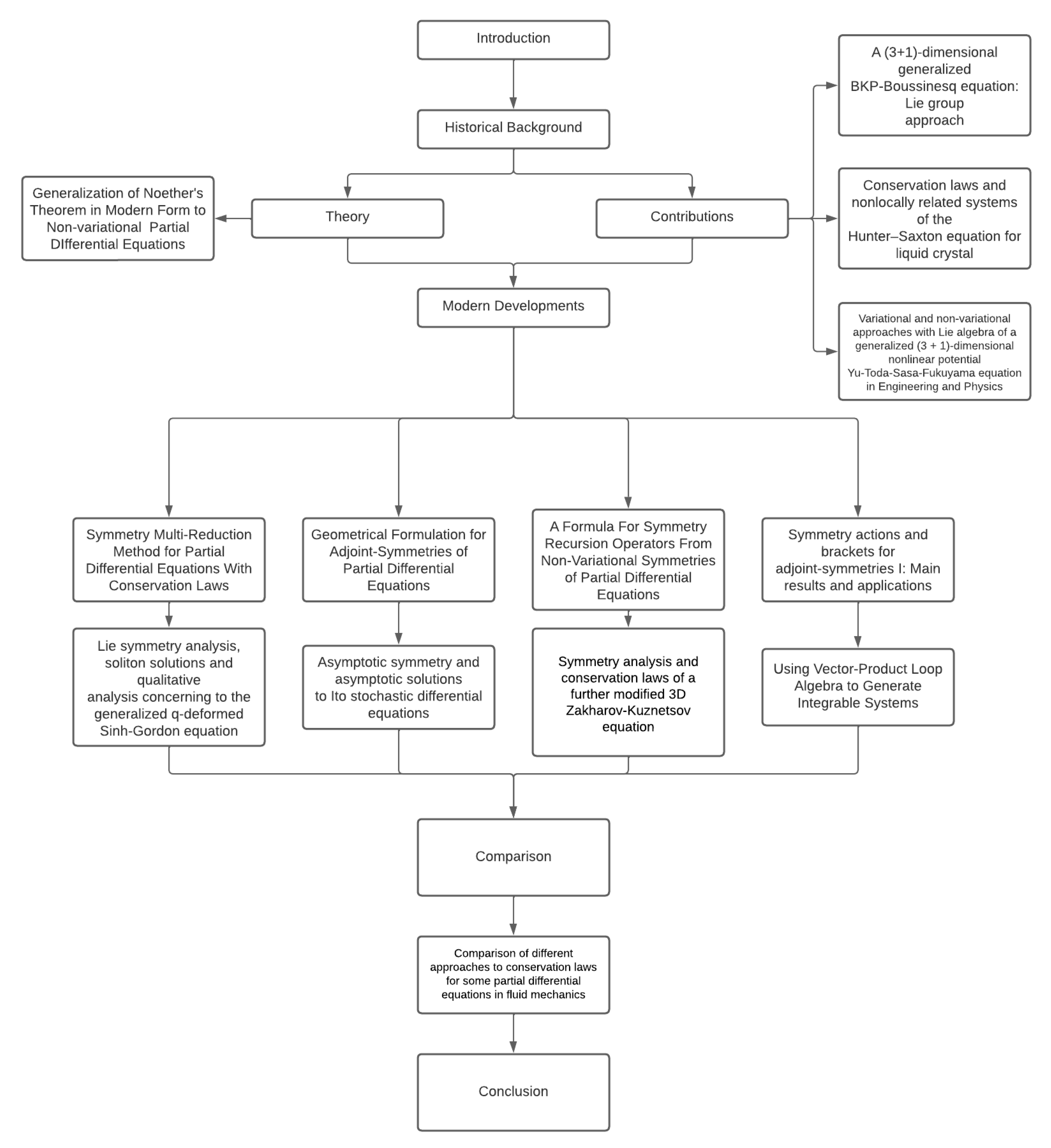
In this section, the information of four papers will be synthesized; each one of them gives a new result in non-related aspects of the same method; therefore, each paper will have its own subsection to explain them in detail.

These subsections will be listed in chronological order from oldest to newest starting from [16], followed by [17,18,19].

The first paper in the list gives a geometrical interpretation of the adjoint-symmetries for PDEs.

The second paper listed relates the method of multipliers with the symmetry multi-reduction method generalizing it.

The third paper listed gives a formula to derive symmetry reduction operators from non-variational symmetries for PDEs.

The last paper is a study of the algebraic structure for general PDE systems.

At the end of each section of this subsection, an example of a relevant use of this new development is presented and briefly discussed for better understanding of the new results.

3.1. Geometrical Formulation for Adjoint-Symmetries of Partial Differential Equations

The geometrical interpretation of an infinitesimal symmetry is well known as the tangent vector field to the solution space of the PDE; having this geometrical interpretation of the infinitesimal symmetries gives a more accessible way for other fields such as physics or applied mathematics to apply and understand this type of symmetry with respect to the PDE system.

This type of geometrical interpretation was not developed for adjoint-symmetries until the publication of the paper underlying this section; as shown later, giving adjoint-symmetries a geometrical interpretation would make it easier to apply this new type of symmetry to any PDE system and would also help to better understand the structure of these mathematical entities.

The geometrical interpretation of adjoint-symmetries was found to be evolutionary one-forms and for evolutionary systems their geometric meaning corresponds to one-forms that are invariant under the flow of the system being studied.

More generally, adjoint-symmetries of the evolution system with spacial constraints are one-forms invariant up to a functional multiplier of normal one-forms related to the constraint equations [16].

To present these results, first we have to write the tools of jet calculus needed in the language of geometrical algebra; we use the following notation recovered from [16].

Independent variables are defined as $x^i$, $i=1,\dots ,n$ and dependent variables are defined as $u^{\alpha }$, $\alpha =1,\dots ,m$. Derivative variables are denoted by the use of subscripts using the following multi-index notation: $I=\{i_1,\dots ,i_N\}$, $u_I^{\alpha }=u_{i_1\cdots i_N}^{\alpha }:={\partial }_{x^{i_1}}\cdots {\partial }_{x^{i_N}}{u}^{\alpha }$, $\left|I\right|=N$; $I=⌀$,$u_I^{\alpha }:=u^{\alpha }$, $\left|I\right|=0$.

Also, the following useful notation is used: ${\partial }^{k}u$ denotes the set ${\left\{u_I^{\alpha }\right\}}_{\left|I\right|=k}$ of all the derivative variables with the order of $k\ge 0$; $u^{\left(k\right)}$ the set ${\left\{u_I^{\alpha }\right\}}_{0\le \left|I\right|\le k}$ is defined as the set of all derivative variables of all orders up to $k\ge 0$. The summation convention for repeated indices is used throughout this section [16].

Jet space J is defined as earlier. A smooth function $u^{\alpha }={\varphi }^{\alpha }\left(x\right):{\mathbb{R}}^n\to {\mathbb{R}}^m$ defines a point in jet space J at any $x^i={\left(x_0\right)}^i$; the values ${\left(u_0\right)}^{\alpha }:={\varphi }^{\alpha }\left(x_0\right)$ and the derivative values ${\left(u_0\right)}_J^{\alpha }:={\partial }_{j_1\cdots {\partial }_{j_N}}{\varphi }^{\alpha }\left(x_0\right)$ for all orders $N\ge 1$ give a map,

$$u^{\alpha }={\varphi }^{\alpha }\left(x\right)\stackrel{x_0}{\to }\left({\left(x_0\right)}^i,{\left(u_0\right)}^{\alpha },{\left(u_0\right)}_j^{\alpha },\dots \right)\in J.$$

(62)

In jet space, the primitive geometric objects consist of partial derivatives ${\partial }_{x^i}$, ${\partial }_{u_j^{\alpha }}$ and differentials $d{x}^i,d{u}_j^{\alpha }.$ These quantities have the following relationship (hooking relations):

$${\partial }_{x_i}\rfloor d{x}^j={\delta }_{i^{\prime }}^j$$

(63)

$${\partial }_{u_I^{\alpha }}\rfloor d{u}_J^{\beta }={\delta }_{\alpha }^{\beta }{\delta }_J^I.$$

(64)

The following geometric contact one-forms will be helpful later:

$${\Theta }_I^{\alpha }=d{u}_I^{\alpha }-u_{I_i}^{\alpha }d{x}^i$$

(65)

Total derivates are given by $D_i=\partial x^i+u_{iJ}^{\alpha }{\partial }_{u_J^{\alpha }}$. Higher total derivatives are defined by $D_J=D_{j_1}\cdots D_{j_N}$, $J=\{j_1,\dots ,j_N\}$, $\left|J\right|=N$.

A differential is defined as a function $f(x,u^{\left(k\right)})$ defined on a finite jet space $J^{\left(k\right)}=(x^i,u^{\alpha },u_j^{\alpha },\dots ,u_{j_i\cdots j_k}^{\alpha })$ of order $k\ge 0$. The Fréchet derivative for a differential function f is defined as

$$f^{\prime }=f_{u_I^{\alpha }}{D}_I$$

(66)

This operator acts on differential functions $F^{\alpha }$. The adjoint Fréchet derivative for a differential function f is defined as

$${\left(f^{\prime \ast }\right)}_{\alpha }={(-1)}^{\left|I\right|}{D}_I{f}_{u_I^{\alpha }}$$

(67)

which also acts on differential functions $F^{\alpha }$.

The second Fréchet derivative is defined as

$$f^{″}(F_1,F_2)=f_{u_I^{\alpha }{u}_J^{\beta }}\left(D_I{f}_I^{\alpha }\right)\left(D_J{F}_2^{\beta }\right).$$

(68)

The Euler operator is defined as

$$E_{u^{\alpha }}={(-1)}^{\left|I\right|}{D}_I{\partial }_{u_I^{\alpha }}.$$

(69)

Higher Euler operators are defined as

$$E_{u^{\alpha }}^I=\left(\genfrac{}{}{0pt}{}{I}{J}\right){(-1)}^{\left|J\right|}{D}_J{\partial }_{u_{IJ}^{\alpha }}.$$

(70)

Fréchet derivatives and Euler operators are related by

$$f^{\prime }\left(F\right)=F^{\alpha }{E}_{u^{\alpha }}\left(f\right)+D_i{\Gamma }^i(F;f),{\Gamma }^i(F;f)=\left(D_J{F}^{\alpha }\right)E_{u_{iJ}^{\alpha }}\left(f\right).$$

(71)

The Fréchet derivative and its adjoint are related by

$$F_2{f}^{\prime }-F_1^{\alpha }{f}^{\prime \ast }{\left(F_2\right)}_{\alpha }=D_i{\Psi }^i(F_1,F_2;f),{\Psi }^i(F_1,F_2;f)=\left(D_K{F}_2\right)\left(D_J{F}_1^{\alpha }\right)E_{u_{iJ}^K}\left(f\right).$$

(72)

A vector field in jet space is defined as

$$P^i{\partial }_{x^i}+P_I^{\alpha }{\partial }_{u_I^{\alpha }}.$$

(73)

A one-form field in jet space is defined as

$$Q_{i}d{x}^i+Q_{\alpha }^{I}d{u}_I^{\alpha }$$

(74)

Geometric partial derivatives ${\partial }_{u_J^{\alpha }}$ can be interpreted as evolutionary vertical differentials $d{u}_J^{\alpha }$, where d is the evolutionary version of d: $d^2=0$, $d{x}^i=0$. These objects satisfy the following duality hooking relations

$${\partial }_{u_I^{\alpha }}\rfloor d{u}_J^{\beta }={\delta }_{\alpha }^{\beta }{\delta }_J^I.$$

(75)

An evolutionary vertical vector field is the geometrical object [16]

$$P_I^{\alpha }{\partial }_{u_I^{\alpha }}.$$

(76)

Its dual counterpart is an evolutionary vertical one-form field,

$$Q_{\alpha }^I$$

(77)

Now, using these definitions and notation we can formulate adjoint-symmetries geometrically, but first we need a general PDE system of order N

$$G^A(x,u^{(}N))=0,A=1,\dots ,M.$$

(78)

where $x^i$, $i=1,\dots ,n$ are the independent variables and $u^{\alpha }$, $\alpha =1,\dots ,m$ are the dependent variables.

Next, we need to define a symmetry as a vector field

$${\mathbf{X}}_P=P^{\alpha }(x,u^{\left(k\right)}){\partial }_{u^{\alpha }}$$

(79)

and the following two determining equations

$$\left(pr{\mathbf{X}}_P{G}^A\right){{|}_{\mathcal{E}}=G^{\prime }{\left(P\right)}^A|}_{\mathcal{E}}=0$$

(80)

called the symmetry determining equation and

$$G^{\prime \ast }{\left(Q\right)}_{\alpha }{|}_{\mathcal{E}}=0$$

(81)

called the adjoint-symmetry determining equation.

The question is whether there is any geometrical entity that describes $Q_A$. It is a good idea to work in a coordinate-free PDE system defined in jet space and this can be done as follows.

The system of equations $(G^1\ast (x,u^{\left(N\right)}),\dots ,G^M(x,u^{\left(N\right)}))=0$ defines a set of M surfaces living in finite space $J^{\left(N\right)}(x,u,\partial u,\dots ,{\partial }^{N}u).$ The total derivatives of these equations $(D^1{G}^1\ast (x,u^{\left(N\right)}),\dots ,D_I{G}^M(x,u^{\left(N\right)}))=0$ defines sets of surfaces living in the higher-derivative finite spaces $J^{(N+|I\left|\right)(x,u,\partial u,\dots ,{\partial }^{N+\left|I\right|}u)}$.

It is known that symmetry vector fields are also tangent vector fields with respect to $\mathcal{E}$. This can be seen explicitly in the identities:

$$d{G}^A={\left(G^A\right)}_{u_I^{\alpha }}d{u}_I^{\alpha }$$

(82)

and

$$G^{\prime }{\left(P\right)}^A=pr{\mathbf{X}}_P{G}^A=pr{\mathbf{X}}_P\rfloor d{G}^A$$

(83)

$d{G}^A$ is the normal one-form to the surfaces $G^A=0$. The symmetry determining Equation (80) gives the result that the prolonged vector field $pr{\mathbf{X}}_P$ vanishes thanks to the normal one-form; this then implies that it is tangent to these surfaces iff ${\mathbf{X}}_P$ is a symmetry of the PDE system.

The normal one-form (82) gives a relationship between a one-form and an adjoint-symmetry via:

$${\omega }_Q=Q_A(x,u^{\left(l\right)})d{G}^A.$$

(84)

An equivalent one-form is obtained by using integration by parts in this equation:

$$Q_{A}d{G}^A=Q_A{\left(G^A\right)}^{\prime }\left(du\right)=G^{\prime \ast }{\left(Q\right)}_{\alpha }d{u}^{\alpha }modtotalD.$$

(85)

In the solution space $\mathcal{E}$, this association between one-forms and adjoint-symmetries gives

$${\omega }_Q{|}_{\mathcal{E}}=0modtotalD.$$

(86)

Using these three results in the following theorem [16].

Theorem 2. 

Adjoint-symmetries describes evolutionary one-forms $Q_{A}d{G}^A$ that functionally vanish in the solution space $\mathcal{E}$ of a PDE system (78).

This was formulated for evolutionary vertical vector fields and evolutionary one-forms; these results are easily reformulated using full vector fields and full one-forms given that

$$Q_{A}d{G}^A{{|}_{\mathcal{E}}={\left(G^A\right)}^{\prime \ast }{\left(Q_A\right)}_{\alpha }|}_{\mathcal{E}}{\Theta }^{\alpha }modtotalD$$

(87)

Then, the determining equation can be expressed in terms of the one-form [16] $Q_{A}d{G}^A{|}_{\mathcal{E}}$ by $E_{{\Theta }^{\alpha }}\left(Q_{A}d{G}^A\right){{|}_{\mathcal{E}}={\left(G^A\right)}^{\prime \ast }\left(Q_A\right)|}_{\mathcal{E}}=0.$

From Theorem 2, a well-known formula is derived; this formula generates a conservation law from a pair consisting of a symmetry and an adjoint-symmetry.

Using these results, the geometrical derivation of three actions of symmetries on adjoint-symmetries are found using Cartan’s formula for the Lie derivative of an adjoint-symmetry one-form (84).

First, from the relation between symmetries and adjoint-symmetries, we need the functional pairing between a symmetry vector field and an adjoint-symmetry one-form that is given by,

$$\langle pr{\mathbf{X}}_P,{\omega }_Q\rangle =\langle pr{P}^{\alpha }{\partial }_{u^{\alpha }},Q_{A}d{G}^A\rangle =\int Q_A{G}^{\prime }{\left(P\right)}^{A}dx.$$

(88)

Using this functional pairing, the next theorem can be stated [16].

Theorem 3. 

Vanishing of the functional pairing (88) for any symmetry (79) and any adjoint-symmetry (81) corresponds to a conservation law

$$D_i{\Psi }^i{(P,Q;G)|}_{\mathcal{E}}=0$$

(89)

holding for the PDE system $G^A=0$, where the conserved current ${\Psi }^i(P,Q;G)$ is given by ${\Psi }^i(P,Q;G)=\left(D_K{Q}_A\right)\left(D_J{P}^{\alpha }\right)E_{u_{iJ}^{\alpha }}\left(G^A\right)$.

Giving the relation between symmetries and adjoint-symmetries.

The action of symmetries on adjoint-symmetries can also be derived in this geometrical formulation noting that for a given PDE system (78), the set of adjoint-symmetries is also linear space, and as shown in [57] symmetries of the PDE system have then three different types of actions in this space.

To derive the first symmetry action, the Lie derivative of an adjoint-symmetry one-form with respect to a symmetry vector field is used [16].

Proposition 1. 

If ${\omega }_Q$ is an adjoint-symmetry one-form (84), namely ${\omega }_Q{|}_{\mathcal{E}}=0$$\left(modtotalD\right)$, then its Lie derivative with respect to any symmetry vector ${\mathbf{X}}_{\mathbf{P}}={\mathbf{P}}^{\mathit{\alpha }}{\mathbf{\partial }}_{{\mathbf{u}}^{\mathit{\alpha }}}$ yields an adjoint-symmetry one-form,

$${\mathcal{L}}_{{\mathbf{X}}_P}{\omega }_Q{{|}_{\mathcal{E}}={\omega }_{S_P\left(Q\right)}|}_{\mathcal{E}}=0\left(\mathit{mod}\mathit{total}D\right)$$

(90)

where

$$S_P{\left(Q\right)}_A=Q^{\prime }{\left(P\right)}_A+R_P^{\ast }{\left(Q\right)}_A$$

(91)

are its components.

The next formula due to Cartan for the Lie derivative is written using the operations d and ⌋. Using this formula, the following two additional symmetry actions are derived [16].

Theorem 4. 

The terms in Cartan’s formula

$${\mathcal{L}}_{{\mathbf{X}}_P}{\omega }_Q=d(pr{\mathbf{X}}_P\rfloor {\omega }_q)+pr{\mathbf{X}}_P\rfloor \left(d{\omega }_Q\right)$$

(92)

evaluated on $\mathcal{E}$ each yield an action of symmetries on adjoint-symmetries. The action produced by the Lie derivative term has the components (91) and the actions produced by the differential term and the hook term, respectively, have the components

$$S_{1P}\left(Q\right)=R_P^{\ast }{\left(Q\right)}_A-R_Q^{\ast }{\left(P\right)}_A^{\prime }$$

(93)

$$S_{2P}\left(Q\right)=Q^{\prime }{\left(P\right)}_A+R_Q^{\ast }{\left(P\right)}_A$$

(94)

The three actions (91), (93) and (94) are related by:

$$S_{1P}\left(Q\right)+S_{2P}\left(Q\right)=S_P{\left(Q\right)}_A$$

(95)

where each of these actions describes a mapping on the linear space of adjoint-symmetries $Q_A$.

The last important result in this paper is the geometrical interpretation of adjoint-symmetries of evolution equations.

To present these results, first a general system of evolution equations of order N is defined as follows

$$u_t^{\alpha }=g^{\alpha }(x,u,{\partial }_{x}u,\dots ,{\partial }_x^{N}u)$$

(96)

where t is taken to be time variable, $x^i$, $i=1,\dots ,n$ are the space variables and $u^{\alpha }$, $\alpha =1,\dots ,m$ are the dependent variables. The space of solutions will still be denoted $\mathcal{E}$.

For general PDE systems, we can specialize them with $G^{\alpha }=u_t^{\alpha }-g^{\alpha }$ via identifying the indices $A=\alpha$$(M=m)$. In $\mathcal{E}$, it is assumed that only $u^{\alpha }$ and its spatial derivatives are contained in addition to t and $x^i$.

A symmetry is then stated to be an evolutionary vector field,

$${\mathbf{X}}_P=P^{\alpha }(t,x,{\partial }_{x}u,\dots ,{\partial }_x^{k}u){\partial }_{u^{\alpha }}$$

(97)

that satisfies the linearization of the evolution system on $\mathcal{E}$:

$$\left(pr{\mathbf{X}}_P(u_t^{\alpha }-g^{\alpha })\right){{|}_{\mathcal{E}}=(D_t{P}^{\alpha }-g^{\prime }{\left(P\right)}^{\alpha })|}_{\mathcal{E}}=0.$$

(98)

The symmetry determining Equation (98) can now be expressed as:

$${(P_t+[g,P])}^{\alpha }=0.$$

(99)

The following determining equation for adjoint-symmetries $Q_{\alpha }(t,x,{\partial }_{x}u,\dots ,{\partial }_x^{l}u)$ is described in terms of the the adjoint linearization of the evolution system in $\mathcal{E}$:

$${(Q_t+Q^{\prime }\left(G\right)+g^{\prime \ast }\ast \left(Q\right))}_{\alpha }=0.$$

(100)

These two determining equations have a geometrical formulation using the Lie derivative defined using the flow that arises from the evolution system; similar work was carried out in [58] for ODEs.

It is useful to introduce the following flow vector field

$$\mathbf{Y}={\partial }_t+g^{\alpha }{\partial }_{u^{\alpha }}$$

(101)

related to the Lie derivative as

$${\mathcal{L}}_t:={\mathcal{L}}_{pr\mathbf{Y}}.$$

(102)

From this relationship, the following well-known result can be stated [16].

Proposition 2. 

A symmetry of an evolution system (96) is an evolutionary vector field (79) that is invariant under the associated flow (102).

In particular, the resulting Lie-derivative vector field

$${\mathcal{L}}_t{\mathbf{X}}_P={(P_t+[g,P])}^{\alpha }{\partial }_{u^{\alpha }}$$

(103)

vanishes iff the functions $P_{\alpha }$ are the components of a symmetry.

For adjoint-symmetries, we introduce the evolutionary one-form

$${\omega }_Q=Q_{\alpha }(t,x,{\partial }_{x}u,\dots ,{\partial }_x^{l}u)d{u}^{\alpha }.$$

(104)

Its Lie derivative is given by

$${\mathcal{L}}_t{\omega }_Q={(Q_t+Q^{\prime }\left(g\right)+g^{\prime \ast }\left(Q\right))}_{\alpha }d{u}^{\alpha }\left(\mathit{mod}\mathit{total}D\right)$$

(105)

Then, the adjoint-symmetry determining Equation (100) can be formulated as the functional vanishing of the Lie derivative expression (105).

Using this proposition, the following theorem is stated [16].

Theorem 5. 

An adjoint-symmetry of an evolution system (96) is an evolutionary one-form (104) that is functionally invariant under the associated flow (105).

In particular, the resulting Lie-derivative one-form

$${\mathcal{L}}_t{\omega }_Q={(Q_t+Q^{\prime }\left(g\right)+g^{\prime \ast }\left(Q\right))}_{\alpha }d{u}^{\alpha }\left(\mathit{mod}\mathit{total}D\right)$$

(106)

functionally vanishes iff the functions $Q_{\alpha }$ are the components of an adjoint-symmetry.

Now, the generalization for evolution equations with spacial constraints is also developed in this paper; this type of system is of high relevance in many areas of physics and applied mathematics; some examples are Maxwell’s equations, incompressible fluid equations, Einstein’s equations, etc.

The constraints consist of spatial equations

$$C^Y(x,u,{\partial }_{x}u,\dots ,{\partial }_x^{N^{\prime }}u)=0,Y=1,\dots ,M^{\prime }$$

(107)

The symmetry equation is described by the linearization of the system on $\mathcal{E}$ and is written as

$$\left(pr{\mathbf{X}}_P{C}^Y\right){{|}_{\mathcal{E}}=C^{\prime }{\left(P\right)}^Y|}_{\mathcal{E}}=0.$$

(108)

The two determining equations (98) and (108) can be stated as:

$${(P_t+[g,P])}^{\alpha }{{|}_{{\mathcal{E}}_C}=0,C^{\prime }{\left(P\right)}^Y|}_{{\mathcal{E}}_C}=0$$

(109)

where ${\mathcal{E}}_C$ is defined as the solution space for the spatial constraint equations.

The determining equation in the adjoint case is found thanks to the adjoint linearization of the full system; this can be stated as:

$${(Q_t+Q^{\prime }\left(G\right)+g^{\prime \ast }\left(Q\right)-C^{\prime \ast }\left(q\right))}_{\alpha }{|}_{{\mathcal{E}}_C}=0.$$

(110)

A geometrical formulation is known in terms of a constrained flow (102) and gives the next generalization of evolutionary systems [16].

Theorem 6. 

A symmetry of a constrained evolution system (96) and (107) is an evolutionary one-form (104) that is functionally invariant under the associated constrained flow (105), up to a functional multiple of the normal one-form $d{C}^Y$ arising from the constraints.

Another theorem is stated in this paper that gives a geometrical result related to gauge adjoint [16,59,60,61].

Theorem 7. 

A gauge adjoint-symmetry ${\omega }_{\chi }=C^{\prime \ast }{\left(\chi \right)}_{\alpha }d{u}^{\alpha }={\chi }_{Y}d{C}^y\mathit{mod}\mathit{total}D$ is functionally equivalent to a normal one-form ${\omega }_{\chi }$ associated with the constraint Equation (107). Under the evolution flow, it is mapped into another normal one-form.

The paper gives some last remarks on what are interesting paths to further develop these results such as working this constraint equation to a formulation using conditional symmetries and conditional adjoint-symmetries based on the spatial constraints of the system.

Translating these results via secondary calculus [62,63], the tool developed by Vinogradov and Krasil’shchik and their coworkers is also advised as an interesting path for further developing the method.

And lastly the authors point out that an interesting path of research would be the full development of the use of adjoint-symmetries for studying specific PDE systems, that is, finding exact solutions, detecting and finding mappings in a target of class of PDEs and detecting integrability of particular PDE systems using this method.

3.2. Example 4 Ito-Type Stochastic Equation

One of the only articles that reference this work, given how recent the work is, is the one found in [64]; here, the asymptotic symmetry and asymptotic solutions for Ito stochastic differential equations are presented.

When finding the conservation laws for these types of equations, similarities were found for the stochastic case and the so-called deterministic ODEs.

The work that we presented earlier only works in terms of deterministic ODEs, while the latter article analyzes stochastic ODEs.

The authors, by trying to find conservation laws for this type of ODE, found a similarity between the geometrical interpretation obtained here and the stochastic ODEs.

To see this more clearly, we will recover the important parts of [64] concerning the results presented here.

First, let us consider the next vector field for a stochastic ODE

$$X=\tau (x,t,\omega )\frac{\partial }{\partial t}+{\varphi }^i(x,t,\omega )\frac{\partial }{\partial x^i}+h^k(x,t,\omega )\frac{\partial }{\partial {\omega }^k}$$

(111)

This equation is then written in the following form if we impose that a certain transformation leaves invariant our vector field, giving a necessary but not sufficient condition for invariance

$$X=\tau \left(t\right)\frac{\partial }{\partial t}+{\varphi }^i(x,t,\omega )\frac{\partial }{\partial x^i}+\left(R_l^k{\omega }^l\right)\frac{\partial }{\partial {\omega }^k}$$

(112)

where R is a matrix that belongs to the Lie algebra of the linear group $CL\left(n\right)$.

Then, an infinitesimal action of X is described as

$$t\to t+ϵ\tau ,x^i\to x^i+ϵ{\varphi }^i,{\omega }^k\to {\omega }^k+ϵR_l^k{\omega }^l.$$

(113)

The equations studied here are Ito-type; this type of equation has the following form

$$d{x}^i=f^i(x,t)dt+{\omega }_k^i(x,t)d{\omega }^k$$

(114)

The infinitesimal action described earlier leaves invariant this type of equation and therefore when applied to Equation (113) we have that

$$d{x}^i={\widehat{f}}^i(x,t)dt+{\widehat{\sigma }}_k^i(x,t)d{\omega }^k$$

(115)

From this equation, we can see that the action of the vector field X is different from the usual way it acts on deterministic ODEs.

The way this vector fields work in deterministic equations is by acting on a proper vector field Z that lives in a suitable jet bundle J of the system; when studying how X and its prolongation acts on Z, we may be able to find the conservation laws of the system.

For the case of stochastic Ito equations, the vector field X acts on the functions $f^i(x,t)$ and ${\sigma }_k^i(x,t)$; therefore, the vector field acts on the differentials $d{x}^i,dt,d{\omega }^k$.

This can be seen in Equation (115) and it looks similar to how vector fields of adjoint-symmetries behave.

This is pointed out in this article and gives an interesting result in terms of how, for two seemingly unrelated types of equations, a bridge between them seems to appear thanks to the use of adjoint-symmetries.

More work needs to be conducted on this point for any strong conclusions, but a connection seems to exist between some stochastic equations and deterministic equations in the sense that the underlying structure of their symmetries seems to be connected thanks to the use of adjoint-symmetries on deterministic equations.

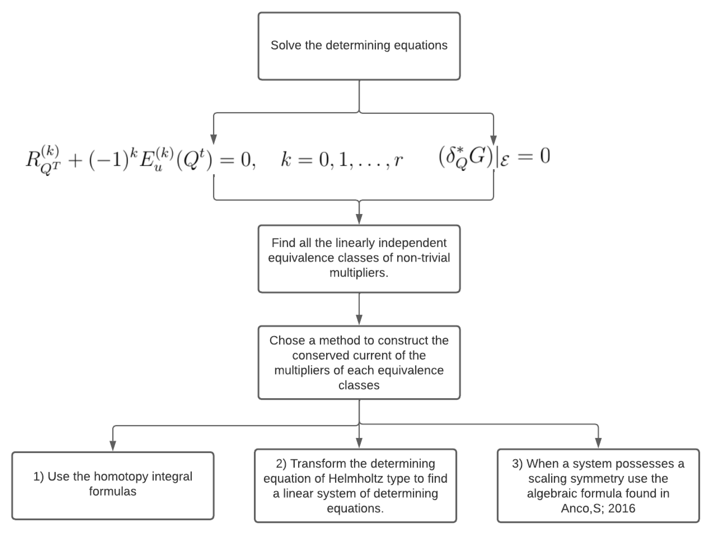
3.3. Symmetry Multi-Reduction Method for Partial Differential Equations with Conservation Laws

This paper [17] gives an algorithmic method for finding all symmetry-invariant conservation laws for PDEs that have $n\ge 2$ independent variables and a symmetry algebra of dimensions of at least $n-1$.

This is a generalization for the well-known double reduction method.

In this paper, the condition for symmetry invariance of a conservation law is given with the use of multipliers; this is because it makes it possible to obtain symmetry-invariant conservation laws in a direct way.

This is done in order to make the calculation steps of this reduction method easier with respect to the number of steps needed and the complexity of these calculations.

In this paper, various examples are presented; these examples will not be added in this review but any extra information can be found in [17].

To understand what the reduction method achieves, it is important to remember that symmetries are used for finding group-invariant solutions of PDEs. When finding these solutions for PDEs, what we obtain is a reduced differential equation (DE) that is expressed using less variables and it is expressed in terms of the invariants that the symmetry group possesses.

By solving this reduced DE, one finds the group-invariant solutions; for us to be able to solve this DE sufficiently, many first integrals are needed so the system can reduce its order for finding the quadrature of the reduced DE.

When the reduced DE obtained is an ordinary differential equation (ODE), we can make further reductions of the system if the system of PDE studied is a Lagrangian one; this is possible thanks to the fact that via Noether’s Theorem we can find a local conservation law that will reduce this ODE to a first integral, giving us the quadrature of this reduced ODE.

The double reduction described earlier for PDEs is a direct counterpart of the double reduction of a variational problem describing an ODE system [65].

The more general reduction method found in [66,67] applies not only to variational PDEs but also to non-variational ones; this method has a long story and it was already developed a decade ago.

This method involves finding an invariant symmetry of the corresponding conserved current in a local conservation law of a PDE.

If the system when reduced under the symmetry specified gives a first integral of the ODE, then it is known that this PDE system has a Lagrangian and this first integral obtained using this method is equal to the one obtained by using the Lagrangian reduction method.

This double reduction method has been extended [68] to PDEs of any number of independent and dependent variables; when carrying out this extension, we find a reduced ODE that describes a PDE having one less independent variable and also an invariant conserved current that is reduced yields a conservation law for this reduced PDE [67]. This can be further extended for conserved currents invariant modulo a trivial current. This extension requires that the underlying local conservation law is invariant [11,69].

In this paper, many applications of the double reduction method are studied [35,66,67,70,71,72,73,74,75,76,77,78].

All of these applications begin by proposing a known conservation law and a known symmetry group for a certain PDE.

Therefore, the method consists of finding a symmetry generator under the conserved current of the given conservation law and this conserved current needs to be strictly invariant or invariant modulo some trivial current.

One problem the method faces is for PDEs that are not of second order; for this type of PDE, the method does not provide sufficient first integrals in order to obtain the quadrature of the PDE.

This paper tries to solve this problem; to do this, first the method does not start by imposing a known conservation law and then working with the symmetries of this conservation law, but instead the method starts by finding the symmetry of the PDE to be used in that case and from this result the conservation laws that are invariant under the symmetry are derived.

This solves the problem for non-second-order PDEs of not having enough first integrals for systems of two independent variables.

Using this approach, further reductions in the ODE are possible.

Second, the reduction in the PDE is considered to be carried out under an algebra of symmetries as opposed to a single symmetry.

This gives a solution for the problem of reducing PDEs with more than two independent variables and gives a reduced system of ODEs with a set of first integrals for finding the quadrature of the system.

Lastly, the condition of symmetry invariance for a given conservation law is written using multipliers; the main goal of this is to make the process algorithmic and therefore make it more straightforward to solve.

Using this approach, the complexity and length of computational steps needed for the reduction method are largely decreased.

We will start with the travelling wave reduction; a travelling wave solution of a PDE $G(t,x,u,u_t,u_x,\dots )=0$ is of the form

$$u(t,x)=U(x-ct)$$

(116)

where $c=const$ is the wave speed. The solutions of this system come from an invariance under a translation symmetry

$$X={\partial }_t+c{\partial }_x$$

(117)

with $x-ct=\xi$ and $u=U$ being the invariants of the symmetry.

The condition of symmetry can then be expressed as

$$prX\left(G\right)=G_t+c{G}_x=0$$

(118)

Invariant solutions satisfy the ODE obtained from reducing the PDE

$${G|}_{u_t+c{u}_x=0}=\overline{G}\left(\xi ,\frac{dU}{d\xi },\dots \right)=0.$$

(119)

The first integrals for this travelling wave ODE (119) are now found via the symmetry reduction of the conservation laws that are invariant under X and are then expressed in terms of $(\xi ,\rho ,U)$ with $X={\partial }_{\rho }$, where $\xi =x-ct,U=u$ is the invariants of the system and the canonical coordinate is given by $\rho =x$. When using these new expressions, the conservation law is then rewritten as

$$\overline{T}=T-\frac{1}{c}\Phi ,\overline{\Phi }=\frac{1}{c}\Phi .$$

(120)

Under the action of $X={\partial }_{\rho }$, the conserved current $(\overline{T},\overline{\Phi })$ is mapped via $\tilde{T}=prX\left(\overline{T}\right)={\partial }_{\rho }\overline{T}$ and $\tilde{\Phi }=prX\left(\overline{\Phi }\right)={\partial }_{\rho }\overline{\varphi }$.

Then, we know that a conservation law is invariant under the travelling wave symmetry iff $(\tilde{T},\tilde{\Phi })$ describes a mapping to a trivial conserved current (see [17]):

$$\tilde{T}=prX\left(\overline{T}\right)={\partial }_{\rho }\overline{T}=D_{\rho }\overline{\Theta },\tilde{\Phi }=prX\left(\overline{\Phi }\right)={\partial }_{\rho }\Phi =-D_{\xi }\overline{\Theta }$$

(121)

This invariance condition (121) is not written in terms of multipliers; as said earlier, formulating this in terms of multipliers gives multiple advantages; the starting point to make this possible is first defining the next mapping of multipliers.

The multiplier mapping $Q\to \tilde{Q}$ is given by [11,69]

$$\tilde{Q}=prX\left(Q\right)+(R_X+D_X\xi +D_t\tau )Q$$

(122)

where $R_X$ is the function defined by $prX\left(Q\right)=R_{X}G$.

Symmetry invariance of a conservation law is a multiplier condition [11,69]

$$\tilde{Q}{|}_{\mathcal{E}}=0.$$

(123)

More details on the derivation of these two expressions can be found in [17].

For the purposes of this paper, we only need these two main results (122) and (123) to rewrite (121) in an equivalent more useful way [17]

$$prX\left(Q\right)=Q_t+c{Q}_x=0$$

(124)

which holds for the multiplier Q of the conserved current $(T,\Phi )$.

From this invariance condition, the next conserved current is derived in terms of canonical variables [17]

$$D_{\xi }\overline{T}+D_{\rho }\overline{\Phi }=D_{\xi }\Psi =0.$$

(125)

This is a reduced conservation law (125) that is a first integral $\Psi =const$ of the travelling wave ODE (119). This conservation can be expressed in an explicit form as

$$\Psi \left(\xi ,U,\frac{dU}{d\xi },\dots \right)=\overline{T}+\int {\partial }_{\rho }\overline{\Phi }d\xi$$

(126)

which only involves the current

$$(\overline{T},\overline{\Phi })=\left(T-\frac{1}{c}\Phi ,\frac{1}{c}\Phi \right){|}_{u(t,x)=U\left(\xi \right),t=\frac{1}{c}(\rho -\xi ),x=\rho }$$

(127)

An equivalent formula for the fist integral can be written as [17]

$$\Psi \left(\xi ,U,\frac{dU}{d\xi },\dots \right)=\int \overline{Q}\overline{G}d\xi$$

(128)

in terms of a multiplier

$$\overline{Q}={\left|J\right|Q|}_{u(t,x)=U\left(\xi \right),t=\frac{1}{c}(\rho -\xi ),x=\rho }$$

(129)

where Q is a multiplier for some symmetry invariant conservation law and $\left|J\right|=\left|\frac{\partial (\xi ,\rho )}{\partial (t,x)}\right|=\frac{1}{c}$ is the Jacobian factor that comes from the point transformation from the normal system variables to the canonical ones $(t,x,u)\to (\xi ,\rho ,U)$.

Then, for any symmetry invariant conservation law for a given PDE $G=0$ will be reduced to a first integral for a travelling wave ODE $\overline{G}=0$; the conservation laws from here can be derived when solving Equations (41) and (124) for Q [17].

The first integrals then can be solved via (126) in terms of $(T,\Phi )$ which comes from the multiplier Q or from Equation (128) which is written in terms of the reduced multipliers (129).

Next is the case of similarity (scaling) reduction; this type of solution of a PDE $G(t,x,u,u_t,u_x,\dots )=0$ takes the form

$$u(t,x)=t^{\alpha }U(x/t^{\beta })\mathrm{or}u(t,x)=x^{\alpha }U(t/x^{\beta })$$

(130)

where $\alpha ,\beta =const$ are scaling weights. Solutions for this type of PDE arise from invariance under a scaling symmetry [17]

$$X=t{\partial }_t+\beta x{\partial }_x+\alpha u{\partial }_u\mathrm{or}X=\alpha t{\partial }_t+x{\partial }_x+\beta u{\partial }_u$$

(131)

The symmetry invariance for this system can be expressed in the solution space $\mathcal{E}$ as [17]

$$prX\left(G\right)=t{G}_t+\beta x{G}_X+\alpha u{G}_u+(\alpha +1)u_t{G}_{u_t}+\cdots =\Omega G$$

(132)

where $\Gamma =const$ represents the scaling weight of the PDE.

The solutions arising from here need to satisfy the reduced ODE corresponding to the PDE.

$$t^{-\Omega }G{|}_{t{u}_t+\beta x{u}_x-\alpha u=0}=\overline{G}\left(\xi ,\frac{dU}{d\xi },\dots \right)=0$$

(133)

The reduction can also be stated in terms of the canonical variables $(\xi ,\rho ,U)$ having the relationship $X={\partial }_{\rho }$, where $\xi =x/t^{\beta }$, $U=u/t^{\alpha }$ are invariants of the system and $\rho =ln\left(t\right)$ is the canonical coordinate.

A conservation law $D_{\xi }\overline{T}+D_{\rho }\overline{\Omega }=0$ is given by

$$\overline{T}=\beta xT-t\Omega ,\overline{\Omega }=t^{\beta }\Omega .$$

(134)

which are functions $\rho ,\xi ,U$ and derivatives of U.

This condition for symmetry invariance can also be written in terms of multipliers for the conserved current $T,\Omega$ as

$$prX\left(Q\right)=t{Q}_t+\beta x{Q}_x+\alpha u{Q}_u+(\alpha -1)u_t{Q}_{u_t}+(\alpha -\beta )u_x{Q}_{u_x}+\cdots =-(\Omega +\beta +1)Q.$$

(135)

from the relations (126) and (125). This gives Equation (128) in terms of multipliers [17]

$$\overline{Q}=\left|J\right|e^{{\Omega }_{\rho }}Q{|}_{u(t,x)=t^{\alpha }U\left(\xi \right),t=e^{\rho },x=e^{\beta }\rho }$$

(136)

where Q is the multiplier of the scaling invariant conservation law; $\left|J\right|=\left|\frac{\partial (\xi ,\rho )}{\partial (t,x)}\right|=e^{(\beta +1)\rho }$ is the Jacobian for the transformation made between the usual coordinates and the canonical coordinates of the system $(t,x,u)\to (\xi ,\rho ,U)$.

Then, we can conclude that all conservation laws of a system of PDEs can be obtained by solving (41) and (135) for Q.

The first integrals can be obtained via (126) and (136) in terms of using the reduced multipliers.

These two multi-reduction methods have a generalization to systems with more independent variables and one symmetry.

These results are further generalized to solvable symmetry algebras. This is possible if the symmetry algebra dimensions are one less than the number of independent variables; if this condition is met, the PDE reduces to an ODE.

In this case, each conservation law of the PDE is described by a first integral of the reduced ODE.

In the paper, two cases with a two-dimensional symmetry algebra in $2+1$ dimensions are discussed.

The first type is a system of line travelling waves and the second type is systems describing line similarity solutions and similarity travelling waves.

To present this, first a discussion on conservation laws, multipliers and symmetries in $2+1$ dimensions is needed.

A local conservation law of a scalar PDE $G(t,x,u,u_x,u_y,\dots )=0$ for $u(t,x,y)$ is a continuity equation $D_{t}T+D_x{\Omega }^x+D_y{\Omega }^y=0$ holding the solution space $\mathcal{E}$, where T is the conserved density and $\Omega =({\Omega }^x,{\Omega }^y)$ is the spatial flux vector. The conserved current is $(T,\Omega )$ [17].

As in the last cases, given a non-trivial conservation law of the PDE $G=0$, this conservation law comes from a multiplier.

In this case, Q is a function of $t,x,,y,u$ and derivatives of u, such that ${Q|}_{\mathcal{E}}$ is non-singular.

The PDE $G=0$ admits a point symmetry $X=\tau (t,x,y,u){\partial }_t+{\xi }^x(t,x,y,u){\partial }_x+{\xi }^y(t,x,y,u){\partial }_y+\eta (t,x,y,u){\partial }_u$. The mapping between multipliers and reduced multipliers $Q\to \overline{Q}$ is given by [11,69]

$$\overline{Q}=prX\left(Q\right)+(R_X+D_X{\xi }^x+D_y{\xi }^y+D_t\tau )Q$$

(137)

where $R_X$ is defined by $prX\left(G\right)=R_{X}G$.

The set given by all symmetry-invariant conservation laws under $\{X_1,X_2\}$ is known to be the subspace of all conservation laws described via the PDE $G=0$.

When the invariant subspace has dimension $m\ge 1$, the reduction method will yield a set of m first integrals for the ODE obtained thanks to the symmetry reduction of $G=0$ [17].

Using this definition, we can first develop the case for the reduction by two translations; this is our first case of line travelling waves.

The line travelling wave is a two-dimensional description of a plane wave. These types of waves are described by [17].

$$u(t,x,y)=U(\mu x+\nu y-t)$$

(138)

where $\mu =const$ and $\nu =const$.

Invariance of a PDE $G(t,x,y,u,u_x,u_y,\dots )=0$ under the pair of commuting translation symmetries

$$X_1=({\mu }^2+{\nu }^2){\partial }_t+\mu {\partial }_x+\nu {\partial }_y,X_2=\nu {\partial }_x-\mu {\partial }_y$$

(139)

holding the solution space of the PDE when written in a solved form for a leading derivative.

Line travelling wave solutions $u=U\left(\xi \right)$ correspond to the reduction $u(t,x,y)\to U\left(\xi \right)$ and satisfy the ODE obtained form reducing the PDE [17].

$$G{|}_{\nu u_x-\mu u_y=0,({\mu }^x+{\nu }^2)u_t+\mu u_x+\nu u_y=0}=\overline{G}\left(\xi ,\frac{dU}{d\xi },\dots \right)=0.$$

(140)

This equation is a consequence of (139) as said earlier, where $\nu u_x-\mu u_y=0$ and $({\mu }^2+{\nu }^2)u_t+\mu u_x+\nu u_y=0$ are known as the invariant surface conditions stating that the action of $X_2\mathrm{and}{X}_1$ on the function (138) vanishes [17].

The first integrals for Equation (140) can be derived using this symmetry reduction method applied to the conservation laws found to be invariant under the action of $X_1\mathrm{and}{X}_2$ of the PDE.

This condition of symmetry invariance can be stated again in term of the canonical variables of the system as

$$(t,x,y,u)\to (\xi ,\rho ,\chi ,u)$$

(141)

given by $\rho =c^{2}t$ and $\chi =c^2(\nu x-\mu y)$ where c is the speed of the wave. This pair of symmetries together written in canonical variables looks as follows

$$X_1={\partial }_{\rho },X_2={\partial }_{\chi },$$

(142)

The transformation (141) then sends a conservation law in normal variables to an equivalent one written in canonical form [17] $D_{\xi }\overline{T}+D_{\rho }{\overline{\Omega }}^{\rho }+D_{\chi }{\overline{\Omega }}^{\chi }=0$, with

$$\overline{T}=\frac{1}{c^2}\left(\mu {\Omega }^x+\nu {\Omega }^y-T\right),{\overline{\Omega }}^{\rho }=Tm{\overline{\Omega }}^{\chi }=\nu {\Omega }^x-\mu {\Omega }^y$$

(143)

The invariance condition rewritten in terms of the conservation law multipliers reads as follows [17]:

$$pr{X}_1\left(Q\right)=({\mu }^2+{\nu }^2)Q_t+\mu Q_x+\nu Q_y=0,pr{X}_2\left(Q\right)=\nu Q_x-\mu Q_y=0,$$

(144)

All conservation laws again can be obtained via (41) and (124).

The formula for the first integrals of this system is then given again by

$$\Psi \left(\xi ,U,\frac{dU}{d\xi },\dots \right)=\overline{T}\int ({\partial }_{\rho }{\overline{\Omega }}^{\rho }+{\partial }_{\chi }{\overline{\Omega }}^{\rho })d\xi$$

(145)

The transformation using canonical variables is written as

$$(\overline{T},{\overline{\Omega }}^{\rho },{\overline{\Omega }}^{\chi })=\left(\frac{1}{c^2}\left(\mu {\Omega }^x+\nu {\Omega }^y-T\right),T,\nu {\Omega }^x-\mu {\Omega }^t\right){|}_{u(t,x,y)=U\left(\xi \right)t=\frac{1}{c^2}\rho ,x=c^2\mu \xi +\mu \rho ,\nu \chi ,y=c^2\nu \xi -\nu \rho +\mu \chi }.$$

(146)

An equivalent multiplier formula is also possible and reads as follows

$$\Psi \left(\xi ,U,\frac{dU}{d\xi },\dots \right)=\int \overline{Q}\overline{G}d\xi$$

(147)

using a reduced multiplier given by

$$\overline{Q}=\left(\right|J\left|Q\right){|}_{u(t,x,y)=U\left(\xi \right)t=\frac{1}{c^2}\rho ,x=c^2\mu \xi +\mu \rho ,\nu \chi ,y=c^2\nu \xi -\nu \rho +\mu \chi }$$

(148)

in terms of the multiplier Q of a symmetry-invariant conservation law with a Jacobian given by $J=\frac{\partial (\xi ,\rho ,\chi )}{\partial (t,x,y)}$

The next part presents results obtained for reduction of scaling and translation symmetries; this type of reduction help to describe line similarity solutions and traveling similarity solutions.

A line solution is a two-dimensional version of a similarity solution (130) with solutions

$$u(t,x,y)=t^{\alpha }U((\mu x+\nu y)/t^{\beta })$$

(149)

This type of solution is invariant under the pair of symmetries of a spatial translation and a scaling [17]

$$X_1=\nu {\partial }_x-\mu {\partial }_y,X_2=t{\partial }_t+\beta x{\partial }_x+\beta y{\partial }_y+\alpha u{\partial }_u$$

(150)

whose joint invariants are $(\mu x+\nu y)/t^{\beta }=\xi$ and $u/t^{\alpha }=U$.

A travelling similarity solution, in contrast, is of the form [17]

$$u(t,x,y)={(\nu x-\mu y)}^{\alpha }U((\mu x+\nu y-t)/{(\nu x-\mu y)}^{\beta })$$

(151)

This type of solution possess the following two invariant pairs of symmetries

$$\begin{array}{cc}\hfill X_1& =({\mu }^2+{\nu }^2){\partial }_t+\mu {\partial }_x+\nu {\partial }_y,\hfill \\ \hfill X_2& =\beta t{\partial }_t+((\beta {\mu }^2+{\nu }^2)x+(\beta -1)\mu \nu y){\partial }_x+(({\mu }^2+\beta {\nu }^2)y+(\beta -1)\mu \nu x){\partial }_y+\alpha u{\partial }_u,\hfill \end{array}$$

(152)

This represents a travelling wave translation and a scaling that is aligned with the translation applied to it; the joint invariants for this are $(\mu x+\nu y-t)/{(\nu x-\mu y)}^{\beta }\xi$ and $u/{(\nu x-\mu y)}^{\alpha }=U$.

The important connection between these two types of solutions is the algebra described by the symmetries; these two symmetries comprise a solvable algebra with the same commutator structure

$$[X_1,X_2]=C{X}_1$$

(153)

where $C=\beta =const$ is known as the structure constant.

The canonical variables $\rho ,\chi$ satisfy $X_1\rho =1$, $X_2\chi =1$. These are not joint canonical coordinates because these two symmetries do not commute.

Imposing the conditions $X_1\chi =0$, $X_2\rho =C\rho$, whereby $X_1={\partial }_{\rho }$, $X_2={\partial }_{\chi }+C\rho {\partial }_{\rho }$ after a point transformation between Q and $\overline{Q}$. This is introduced to help carry out the reduction method as similarly as possible to the other cases.

The relevant details that make important the study of algebras with a solvable structure of the symmetry algebra are the condition symmetry invariance (152) of multipliers

$$0=({\mu }^2+{\nu }^2)Q_t+\mu Q_x+\nu Q_y$$

(154)

$$\begin{array}{c}CQ=\beta t{Q}_t+((\beta {\mu }^2+{\nu }^2)x+(\beta -1)\mu \nu y)Q_x+(({\mu }^2+\beta {\nu }^2)y+(\beta -1)\mu \nu x)Q_y+\alpha u{Q}_u+\hfill \\ \hspace{1em}\hspace{1em}\hspace{1em}\hspace{1em}\hspace{1em}\hspace{1em}\hspace{1em}\hspace{1em}\hspace{1em}\hspace{1em}\hspace{1em}\hspace{1em}\hspace{1em}\hspace{1em}\hspace{1em}\hspace{1em}\hspace{1em}\hspace{1em}\hspace{1em}\hspace{1em}\hspace{1em}\hspace{1em}\hspace{1em}\hspace{1em}\hspace{1em}\hspace{1em}\hspace{1em}\hspace{1em}\hspace{1em}\hspace{1em}\hspace{1em}\cdots +(\Omega +\beta +2)Q=CQ\hfill \end{array}$$

(155)

where $\Omega =const$ is known as the scaling weight of the PDE.

The second invariance condition has an extra term $CQ$; this term cancels the $\beta Q$ term.

This term is related to the solvable structure of the symmetry algebra; this element vanishes in the abelian case, $C=0$ [17].

The first integral formulas are the same as (145), (147) and (148) derived in the abelian case $C=0$ [17].

Lastly, in this paper the multi-reduction under a non-solvable symmetry algebra is mentioned and some examples are given; the theory is related to other studies in the literature.

The important remark is that the theory developed for solvable symmetries can also be generalized to non-solvable algebras with some conditions.

For a reduction in a PDE with n independent variables and an ODE with the same number of independent variables, we need to impose conditions on the algebra; specifically, the algebra needs to have two invariants; one of these invariants needs to involve the dependent variable of the PDE. For a more formal treatment of this case, see [79]. As in the solvable case, the ODE inherits for each symmetry one first integral.

Thanks to these first integrals that are functionally independent, one can further reduce the ODE.

The following is a summary of each case. For the case of a PDE system with two independent variables, from a point symmetry an algorithmic approach was found to obtain all symmetry-invariant conservation laws; these objects are then reduced to first integrals of the reduced ODE describing the symmetry-invariant solutions of the PDE.

This is the generalization given in this paper for the double reduction method known in literature.

The multi-reduction method is then generalized to PDEs with $n>2$ independent variables and a symmetry algebra of dimension $n-1$.

For this case, the method provides a way of obtaining a direct reduction from a PDE to an ODE for a given invariant solution and also a set of first integrals to find the quadrature of the system.

The symmetry algebras do not need to be solvable. The condition of symmetry invariance is also formulated using multipliers, giving an algorithm for finding theses reductions and also giving the invariance condition of the conservation law in the process.

The third result is related to symmetry-invariant conservation law spaces with dimensions of $m\ge 1$; this method yields m first integrals knowing if they are trivial or non-trivial thanks to the multipliers.

Next, work in the making [79] gives a method for finding all conservation laws inherited by a PDE in fewer variables obtained via symmetry reduction of a PDE in more than two independent variables.

The work presented here is completely new and results and examples of how it is used are found in [17].

Before jumping to the next section, an example of how these results have been used is found in [44].

3.4. Example 5 (q-Deformed Sinh–Gordon)

Here, for the generalized q-deformed Sinh–Gordon equation, the traveling wave reductions were derived; this was achieved with the help of the results presented earlier.

The authors retrieved the reduction found in this paper to find in an easier way the conservation laws of these traveling wave reductions of the equation.

To present these results, first the q-deformed Sinh–Gordon equation is presented as reported in [80,81]

$$\frac{{\partial }^{2}y}{\partial x^2}-\frac{{\partial }^{2}y}{\partial t^2}={\left[{sinh}_n\left(y^{\gamma }\right)\right]}^p-\delta$$

(156)

with ${sinh}_q$ defined as the Arai q-deformed function

$${sinh}_n\left(x\right)=\frac{e^x-n{e}^{-x}}{2};0<n\le 1.$$

(157)

The low-order multipliers are found thanks to the work presented earlier for travelling wave solutions and in this case are given by

$$\begin{array}{cc}\hfill Q1& =\frac{v_t}{v^4},\hfill \\ \hfill Q_2& =\frac{v_x}{v^4},\hfill \\ \hfill Q_3& =t\frac{v_x}{v^4}+x\frac{v_t}{v^4},\hfill \end{array}$$

(158)

These multipliers then produce non-trivial conservation laws of low order

$$\begin{array}{cc}\hfill T_1& =\frac{1}{3v^3}(3v^2+(-3v_t^2-3v_x^2-3\delta )v-n)\hfill \\ \hfill X_1& =\frac{2v_t{v}_x}{v^2}\hfill \end{array}$$

(159)

$$\begin{array}{cc}\hfill T_2& =-\frac{2v_t{v}_x}{v^2}\hfill \\ \hfill X_2& =\frac{1}{3v^3}(3v^2+(-3v_t^2+3v_x^2-3\delta )v-n)\hfill \end{array}$$

(160)

$$\begin{array}{cc}\hfill T_3& =\frac{1}{3v^3}(3x{v}^2+((-3v_t^2-3v_x^2-3\delta )x-6v_{x}t{v}_t)v-xn)\hfill \\ \hfill X_3& =\frac{1}{3v^3}(3t{v}^2+((3v_t^2+3v_x^2-3\delta )t+6v_{t}x{v}_x)v-tn)\hfill \end{array}$$

(161)

This is given in the original variables t, x and y.

Next, the form in canonical variables is given as

$$\begin{array}{cc}\hfill Q_1& =y_t,\hfill \\ \hfill Q_2& =y_x,\hfill \\ \hfill Q_3& =t{y}_x+x{y}_t,\hfill \end{array}$$

(162)

These multipliers give the next non-trivial conservation laws of low order

$$\begin{array}{cc}\hfill T_1& =-\frac{1}{2}(y_x^2+y_t^2)-\int {sinh}_n\left(y\right)dy\hfill \\ \hfill X_1& =y_t{y}_x\hfill \end{array}$$

(163)

$$\begin{array}{cc}\hfill T_2& =-y_t{y}_x\hfill \\ \hfill x_2& =-y_t{y}_x\hfill \end{array}$$

(164)

$$\begin{array}{cc}\hfill T_3& =-t{y}_t{y}_x-\frac{1}{2}(x{y}_t^2-x{y}_x^2)-\int x{sinh}_n\left(y\right)dy\hfill \\ \hfill X_3& =x{y}_t{y}_x+\frac{1}{2}(t{y}_t^2+t{y}_x^2)-\int t{sinh}_n\left(y\right)dy\hfill \end{array}$$

(165)

Then, we have already found all the conservation laws permitted by the generalized q-deformed Sinh–Gordon equation using the reduction method for travelling wave solutions.

This demonstrates the power this new reformulation of the multi-reduction method has in terms of multipliers.

In the paper, several type of solutions for different types of systems are presented and can be applied to more systems that check the necessary conditions imposed here.

As a further remark, the generalized q-deformed Sinh–Gordon equation is widely used in many applications respecting the modelling of complex wave mechanics.

The graphics of the periodic solutions for this system are found in [44].

3.5. A Formula for Symmetry Recursion Operators from Non-Variational Symmetries of Partial Differential Equations

This paper [18] gives an explicit formula for finding symmetry recursion for PDEs; these results are given via a newfound connection between variational integrating factors and non-variational symmetries.

The formula obtained in this paper is found to be a special case of an already-existing general formula that exists for pre-symplectic operators that arise from a non-gradient adjoint-symmetry.

The paper also gives a classification for quasilinear second-order PDEs that admit a multiplicative symmetry recursion operator.

These symmetry recursion operators are really important for the theory of linear PDEs and nonlinear integrable PDEs.

These symmetry recursion operators in the linear case are typically derived using the Fréchet derivative of a Lie symmetry that is written in characteristic form.

In the case of integrable evolution PDEs, another symmetry recursion operator is found using the ratio of two compatible Hamiltonian operators.

The main result of this paper gives a symmetry recursion operator arising in a similar way as in linear PDEs for nonlinear integrable PDEs.

Also, a simple explicit formula for a symmetry recursion operator of a Euler–Lagrange PDE is obtained.

This result is related to all the other research carried out on the method of multipliers because the formula uses the Fréchet derivative of a non-variational symmetry of the PDE, this gives a new use for non-variational symmetries, the same symmetries studied in previous papers.

One important thing to note is that the generalized pre-symplectic operator derived here uses adjoint-symmetries that do not necessarily need to be multipliers of the system.

For Euler–Lagrange PDEs, it is found that the generalized pre-symplectic operator mentioned earlier is equivalent to a symmetry recursion operator; also in this case the non-multiplier adjoint-symmetries of the system are found to be equivalent to non-variational symmetries.

For PDEs with no variational structure, a generalized pre-symplectic operator [82] is found to be a linear differential operator that gives a map between symmetries and adjoint-symmetries, analogously to the case of Hamiltonian evolution equations [83].

The systems studied in this paper are scalar PDEs $G=0$ of any order $N\ge 1$, with n independent variables $x=(x^1,\dots ,x^n)$ and a single dependent variable u.

The space of solutions will be again denoted $\mathcal{E}$. Most of the results in the first review paper will be used for all these new developments and some new concepts will need to be added as in [18].

Definition 1. 

A PDE $G=0$ is a Euler–Lagrange equation, $G=E_u\left(L\right)$, with a Lagrangian given by a differential function L, iff the Fréchet derivative of G is self-adjoint $G^{\prime }=G{″}^{\ast }$.

The next lemma is also useful.

Lemma 6. 

Any Euler–Lagrange PDE $G=E_u\left(L\right)=0$ that is quasilinear and of second order possesses a Lagrangian L that is of first order.

The definition of pre-symplectic operators [82].

Definition 2. 

A generalized pre-symplectic operator is a linear differential operator (in total derivatives) that maps symmetries into adjoint-symmetries.

For pre-Hamiltonian operators [82].

Definition 3. 

A generalized pre-Hamiltonian operator is a linear differential operator (in total derivatives) that maps adjoint-symmetries into symmetries.

When this operator is a pre-Hamiltonian operator, it gives rise to a recursion operator that acts on (adjoint) symmetries.

As said earlier, to derive the new results for a general PDE $G=0$ we need to state the next connection that exist between variational integrating factors, symmetries and adjoint-symmetries [18].

Proposition 3. 

If $G=0$ admits a variational integrating factor W, then for any symmetry ${\widehat{X}}_P=P{\partial }_u$ (in characteristic form) of $G=0$, there is an adjoint-symmetry $Q=WP$.

The mapping $P\to Q=WP$ can be iterated when $G=0$ is Euler–Lagrange, since adjoint-symmetries coincide with symmetries giving that [18].

Proposition 4. 

If $G=0$ is Euler–Lagrange and admits a variational integrating factor W, then starting from any symmetry ${\widehat{X}}^{\left(l\right)}=W^{l}P{\partial }_u$, $l=0,1,2,\dots$. Thus, W is a multiplicative recursion operator for symmetries.

From this, the following necessary condition on G is deduced [18].

Proposition 5. 

A Euler–Lagrange PDE $G=E_u\left(L\right)=0$ admits a non-constant variational integrating factor only if

$$rank\left(\left(\left(\genfrac{}{}{0pt}{}{i_1{i}_2\dots i_N}{i_1}\right)G_{u_{i_1{i}_2\dots i_N}}\right){|}_{\mathcal{E}}\right)\le n-1$$

(166)

This rank condition (166) constitutes an equation of the form of G. For the case when G is of second order, that is $N=2$, the rank condition is equivalent to

$$det{\left(\left({\delta }_{ij}+1\right)G_{u_{ij}}\right)}_{\mathcal{E}}=0.$$

(167)

When G is quasilinear by Lemma 6, the Lagrangian for G can be assumed to have the form $L(x,u^{\left(1\right)})$, so that $G=E_u\left(L\right)=L_u-L_{x^i{u}_i}-u_i{L}_{u{u}_i}-u_{ij}{L}_{u_j{u}_i}$. Then, we have $G_{u_{ij}}=-L_{u_i{u}_j}$, which can be used to express (167) in terms of L:

$$det\left(L_{u_i{u}_j}\right)=0$$

(168)

From here, we obtain the following result [18].

Proposition 6. 

If a quasilinear second-order Euler–Lagrange PDE $G=E_u\left(L\right)$ admits a non-constant variational integrating factor, then the first-order Lagrangian satisfies the Monge–Ampere Equation (168).

For the case of general Euler–Lagrange PDEs, if there exist a non-variational Lie point symmetry of the system then an explicit formula for a variational integrating factor can be derived [18].

Proposition 7. 

Suppose a Euler–Lagrange equation $G=0$ possesses a non-variational Lie point symmetry $X_p=\xi {(x,u)}^i{\partial }_{x^i}+\eta (x,u){\partial }_u$. Then, $G=0$ possesses a variational integrating factor

$$W=f_p+{\eta }_u+{\xi }_{x^i}^i$$

(169)

with $f_p$ defined by

$$pr{X}_p\left(G\right)=f_{p}G.$$

(170)

If this function (169) is non-constant, then it defines a non-trivial multiplicative recursion operator for the symmetries of $G=0$.

To fully state the results of the paper, first a classification is made for non-trivial variational integrating factors and for quasilinear second-order Euler–Lagrange equations in two independent variables [18].

Theorem 8. 

Suppose

$$G\left(u^{\left(2\right)}\right)=A_1\left(u^{\left(1\right)}\right)u_{tt}+A_2\left(u^{\left(1\right)}\right)u_{tx}+A_3\left(u^{\left(1\right)}\right)u_{xx}+A_0\left(u^{\left(1\right)}\right)=0$$

(171)

is a Euler–Lagrange PDE, which is quasilinear and translation invariant. If it admits a variational integrating factor $W(t,x,\left(u^{\left(2\right)}\right))$ that is not a constant, then it is equivalent (modulo a point transformation) to one of the following PDEs:

$$\begin{array}{cc}\hfill \left(a\right)& A_1=\frac{f(u,v)v^2}{u_t},A_2=-2\frac{f(u,v)v}{u_t},A_3=\frac{f(u,v)}{u_t},A_0=0\mathrm{or}0,\hfill \\ \hfill & v=\frac{u_x}{u_t};f(u,v)\mathit{arbitrary}\hfill \end{array}$$

(172)

$$\begin{array}{cc}\hfill \left(b\right)& A_1=\frac{f(u,v)g{\left(u\right)}^2}{v},A_2=2\frac{f(u,v)g\left(u\right)}{v},A_3=\frac{f(u,v)}{v},\hfill \\ \hfill & A_0=f_u(u,v)+f_v(u,v)g_u\left(u\right)u_t,\hfill \\ \hfill & v=g\left(u\right)u_t+u_x;g\left(u\right),f(u,v)\mathit{arbitrary}\hfill \end{array}$$

(173)

$$\begin{array}{cc}\hfill & A_1=\frac{f_v(u,v)v^2}{(g_v(u,v)-u_t)(u_x+v{u}_t)},A_2=2\frac{f_v(u,v)v}{(g_v(u,v)-u_t)(u_x+v{u}_t)},\hfill \\ \hfill & A_3=\frac{f_v(u,v)}{(g_v(u,v)-u_t)(u_x+v{u}_t)},A_0=f_u(u,v)+\frac{f_v(u,v)g_u(u,v)}{(g_v(u,v)-u_t)},\hfill \\ \hfill & v=h(u,u_t,u_x),v{u}_t+u_x=g(u,v);f(u,v),g(u,v)\mathit{arbitrary}\hfill \end{array}$$

(174)

The corresponding variational integrating factors are given by

$$\begin{array}{cc}\hfill \left(a\right)& W=F(u,x+h_1(u,v),t-h2(u,v))\hfill \\ \hfill & h_1(u,v)=\int f(u,v)du+k_1\left(u\right),h2(u,v)=\int vf(u,v)dv+k_2\left(u\right),\hfill \end{array}$$

(175)

$$\begin{array}{cc}\hfill (b,c)& W=F(f(u,v),x-h_1(u,f(u,v)),t-h2(u,f(u,v))),\hfill \\ \hfill & h_1(u,w)=\int \frac{1}{f_{-1}(u,w)}du+k_1\left(w\right),h_2(u,w)=\int g\left(u\right)h_{1u}(u,w)du+k_2\left(w\right),\hfill \\ \hfill & f(u,f^{-1}(u,w))=w;k_1\left(w\right),k_2\left(w\right)\mathit{arbitrary}\hfill \end{array}$$

(176)

where F is an arbitrary function of its arguments. In each case, $W=F$ is a multiplicative recursion operator for symmetries of the corresponding PDE.

The next remarks are important for understanding this type of PDE system [18]

Remark 1. 

1.

A Lagrangian for the PDEs (a)–(c) can be obtained either from the homotopy formula

$$L={\int }_0^{1}uG(x,\lambda u^{\left(2\right)})d\lambda$$

(177)

or integration of the equations $A_1=-L_{u_t{u}_t}$, $A_2=-2L_{u_t{u}_t}$, $A_3=-L_{u_x{u}_x}$, $A_0=L_u-L_{u{u}_t}{u}_t-L_{u{u}_x}{u}_x$.

2.

Each PDE (a)–(c) possesses a sequence of contact symmetries ${\widehat{X}}^{\left(l\right)}=W^{l}P{\partial }_u$, $l=0,1,2,\dots$, starting from the translation symmetry given by $P=a{u}_t+b{u}_x$, where $a,b$ are arbitrary constants.

3.

All of the PDEs (a)–(c) are of a parabolic type, since their coefficients satisfy the algebraic relation $A_2^2-4A_1{A}_3=0$.

4.

None of these PDEs can be mapped into the linear parabolic PDE $u_{tt}\pm 2u_{tx}+u_{xx}=0$ by a contact transformation.

A complete proof of Theorem 8 is found in [18] and we highly encourage the reader to review this proof.

These results can be generalized to yield non-multiplicative operators [18].

Theorem 9. 

Suppose $G=0$ possesses an adjoint-symmetry Q that is not a multiplier, namely

$$G^{\prime \ast }\left(Q\right)=R_Q\left(G\right),E_u\left(QG\right)\not\equiv 0$$

(178)

holds for $\mathcal{E}$, where $R_Q$ is a non-zero linear differential operator in total derivatives whose coefficients are non-singular differential functions on $\mathcal{E}$. Then

$$S:=R_Q^{\ast }+Q^{\prime }$$

(179)

is a linear differential operator in total derivatives that maps symmetries to adjoint-symmetries. Moreover, when an inverse $S^{-1}$ exists, it maps adjoint-symmetries to symmetries.

Such adjoint-symmetry is a multiplier for a conservation law [18].

Proposition 8. 

For a symmetry ${\widehat{X}}_P=P{\partial }_u$ of $G=0$, the adjoint-symmetry $S\left(P\right)$ is a multiplier yielding a conservation law of $G=0$ iff

$$(pr{\widehat{X}}_P{S}^{\ast }+S^{\ast }{R}_P+P^{\prime \ast }{S}^{\ast })G=0$$

(180)

holds for $\mathcal{E}$.

These results applied to an evolution system yield the following result [18].

Theorem 10. 

Suppose $u_t=g$ has an adjoint-symmetry Q that is not a multiplier. Then, the linear differential operator (179), under which symmetries are mapped into adjoint-symmetries, has the skew-symmetric form

$$S=Q^{\prime }-Q^{\prime \ast }=-S^{\ast }$$

(181)

For a symmetry ${\widehat{X}}_P=P{\partial }_u$, the adjoint-symmetry $S\left(P\right)$ is a multiplier, yielding a conservation law, if and only if

$$pr{\widehat{X}}_{P}S+S{P}^{\prime }+P^{\prime \ast }S=0.$$

(182)

For Euler–Lagrange equations, adjoint-symmetries are also symmetries. In this case, the pre-symplectic operator (179) becomes a recursion operator for symmetries [18].

Theorem 11. 

Suppose a Euler–Lagrange equation $G=0$ possesses a symmetry ${\widehat{X}}_P=P{\partial }_u$ that is not variational, namely

$$G^{\prime }\left(P\right)=R_P\left(P\right),E_u\left(PG\right)\not\equiv 0$$

(183)

holds for $\mathcal{E}$, where $R_P$ is non-zero linear differential operator in total derivatives whose coefficients are non-singular differential functions on $\mathcal{E}$. Then

$$S:=R_P^{\ast }+P^{\prime }$$

(184)

is a linear differential operator that maps symmetries to symmetries.

The symmetry recursion operator (184) is a recursion operation applied to variational symmetries when the following applies.

Proposition 9. 

If $P{\partial }_u$ is a variational symmetry of the Euler–Lagrange equation $G=0$, then $S\left(P\right){\partial }_u$ is also a variational symmetry of $G=0$ if and only if

$$[S^{\ast },P^{\prime \ast }]=\left(pr{X}_P{S}^{\ast }\right)G.$$

(185)

Remark 2. 

Given that variational symmetries of Euler–Lagrange equations are the same as a conservation law multiplier by Noether’s Theorem, the condition (185) is necessary for the operator (184) to define a recursion operator on a conservation law multiplier. The condition is sufficient if it holds with $S\left(P\right)$ in place of P.

To compare this with Proposition 7 the case when P is a characteristic function for a given Lie point symmetry is taken into account [18].

Corollary 1. 

If $P=\eta (x,u)-{\xi }^i(x,u)u_i$ is the characteristic function of a non-variational Lie point symmetry of a Euler–Lagrange equation $G=0$, then the corresponding symmetry recursion operator (184) is $S=W$, where W is the variational integrating factor.

Therefore, recursion operators (184) need more than Lie point symmetries.

This is stated in the next corollary [18].

Corollary 2. 

If $P(x,u^{\left(1\right)})$ is the characteristic function of a non-variational contact symmetry of a Euler–Lagrange equation $G=0$, with $pr{X}_{P}G=fG$, then the corresponding symmetry recursion operator (184) is

$$S=f+P_u-D_i{P}_{u_i}$$

(186)

which is a variational integrating factor.

This paper then gives a new form to derive generalized pre-sympletic operators for PDEs, either for the linear or nonlinear systems.

This result also gives new recursion operators for the case of Euler–Lagrange PDEs; these recursion operators work only with non-variational symmetries.

This work can be followed by studying system of PDEs with any number of dependent variables; the authors say they will work in a classification of non-variational symmetries and adjoint-symmetries for interesting classes of PDEs.

The authors also state that a geometrical formulation of these formulas will be studied.

For this paper, the most recent article using these results can be found in [84]; in this work, the Zakharov–Kuznetsov (ZK) equation is studied.

Firstly, the conservation laws of this equation are found via the method of multipliers and other similar methods but the relevant use of the results presented here is the study of the Hamiltonian structure of the target equation.

A generalized pre-symplectic structure is also found; this structure gives a map between symmetries and adjoint-symmetries.

The details are not presented here but for more details we encourage the reader to check the work carried out in [84].

3.6. Symmetry Actions and Brackets for Adjoint-Symmetries I: Main Results and Applications

Note that the second part of this paper will not be discussed here because it contains only examples of the results for this paper and in this review only the theory is presented; the second part of the paper can be found in [20].

In this paper, the algebraic structure of the adjoint linearization equation that holds on the space of solutions to the PDE, also called adjoint-symmetries, is studied.

This work was motivated by the already known relationship that exists between symmetries and adjoint-symmetries.

Several main results are obtained such as the three different linear actions on the linear space of adjoint-symmetries of symmetries.

In this paper, these three new actions found are then used for a construction of bilinear adjoint-symmetry brackets; it is found that one of these brackets describes the pull-back of a symmetry that also has a Lie bracket structure.

The brackets obtained in this paper do not need any local variational structure.

Also, it is found that the last of the symmetry actions derived has a pre-symplectic (Noether) operator encoded; from this bracket, one can then construct a symplectic two-form and also Poisson brackets only for evolution systems.

Note that in the context of Hamiltonian and integrable systems the multipliers are also referred to as cosymmetries [85,86].

The existence of an adjoint-symmetry for a given PDE is also known in this context as “nonlinear self-adjointness” [27].

This paper is a follow-up to the one presented before [18]; in this paper, scalar PDEs were studied to find a linear mapping from infinitesimal symmetries into adjoint-symmetries for any fixed adjoint-symmetry that is not a multiplier.

This mapping was found to be equivalent to a pre-symplectic operator (Noether) and there exists an analog of this case for the mapping between symmetries and adjoint-symmetries that exist in Hamilton systems thanks to symplectic operators [87].

The inverse of this mapping is then found to be a pre-Hamiltonian operator.

This paper then expands on these ideas, but for general PDE systems as opposed to only scalar PDEs.

More specifically, the results of this work first show the existence of two different actions of infinitesimal symmetries on adjoint-symmetries.

The first action is found to be a Lie derivative; the second action arises from the adjoint relationship that exists between the determining equation for infinitesimal symmetries and adjoint-symmetries.

If an adjoint-symmetry is also a multiplier, it was found that the two actions mentioned earlier are the actions of symmetries on the multipliers of the system defined in [11,69,88].

The difference between these two actions also describes a third action that vanishes if the adjoint-symmetry is a multiplier.

This third action is a generalization of the pre-symplectic operator for scalar PDEs; the inverse of this action gives the general pre-Hamiltonian operator.

When considering PDEs and Euler–Lagrange PDEs, this action describes a symplectic two-form that has an associated Poisson bracket; these results are expected to be useful in describing a Hamiltonian structure for non-dissipative PDE systems.

These three actions are used to construct bracket structures on the subset of adjoint-symmetries.

The first bracket constructed in the paper is non-symmetric and is the pull-back of the symmetry commutator; it is also a Lie bracket to adjoint-symmetries; the second bracket constructed is also non-symmetric and it does not use the commutator structure of symmetries.

One of these brackets also satisfies the Jacobi identity; therefore, this bracket also encodes a Lie algebra structure to a natural subset of adjoint-symmetries.

A correspondence is also shown to exist between Lie subalgebras of symmetries and adjoint-symmetries; this correspondence holds for dissipative PDEs with no local variational structure.

The lie bracket that exists on adjoint-symmetries is also found to give a bracket structure to conservation laws; this bracket is found to be a Poisson bracket for non-Hamiltonian systems.

The importance of these results resides in giving a more broad understanding of the basic algebraic structure of adjoint-symmetries and how they apply to pre-Hamiltonian operators, (Noether) pre-symplectic operators and symplectic 2-forms for general PDE systems.

One more important possible use of the results on this paper is to obtain new adjoint-symmetries via the symmetry actions; these actions of symmetries over adjoint-symmetries can give a new adjoint-symmetry and possibly a new multiplier.

This can give rise to new possible conservation laws from adjoint-symmetries that can be or not be a multiplier of the PDE system.

It is known that from a pair of known symmetries one can find a new symmetry from their Lie bracket; therefore, studying these structures for adjoint-symmetries can prove useful for finding new symmetries of a system in an easier way.

The first important result is the action of symmetries on adjoint-symmetries; to state this first we need the well-known fact that symmetries of any given PDE system form a Lie algebra via their commutators.

From the algebraic viewpoint, if $P_1^{\alpha }$, $P_2^{\alpha }$ are symmetries, then it is the commutator defined by [19]

$$[P_1,P_2]\alpha =P_2^{\prime }{\left(P_1\right)}^{\alpha }-P_1^{\prime }{\left(P_2\right)}^{\alpha }.$$

(187)

The geometrical formulation is given by:

$$[pr{X}_{P_1},pr{X}_{P_2}]=pr{X}_{P_1,P_2}.$$

(188)

The set of symmetries for a system is known to be a linear space with a bilinear antisymmetric bracket defined by the commutator that obeys the Jacobi identity.

The bracket is called the Lie bracket of the symmetry vector fields. Symmetries have a natural action on the set of adjoint-symmetries.

The first symmetry action comes from the prolonged action for a symmetry $P^{\alpha }$ of the adjoint-symmetry determining Equation (46).

Carrying out this prolongation, one obtains [19]

$$G^{\prime \ast }{(Q^{\prime }\left(P\right)+R_P^{\ast }\left(Q\right))}_{\alpha }{|}_{\mathcal{E}}=0$$

(189)

This yields a linear mapping

$$Q_A\stackrel{X_P}{\to }{Q}^{\prime }{\left(P\right)}_A+R_P^{\ast }{\left(Q\right)}_A$$

(190)

that acts on the linear space of adjoint-symmetries.

The action (190) geometrically represents the Lie derivative [16] and gives a generalization for a known action of symmetries on the conservation law multipliers of the system.

The second symmetry action is derived from an adjoint relation between the determining Equations (34) and (46), giving the next expression [19]

$$D_i{\Psi }^i(P,Q)=(R_P^{\ast }{\left(Q\right)}_A-R_Q^{\ast }{\left(P\right)}_A)G^A+D_i{F}^i(P,Q;G)$$

(191)

Hence, $(R_P^{\ast }{\left(Q\right)}_A-R_Q^{\ast }{\left(P\right)}_A)G^A$ is a total divergence in jet space; therefore, the set of functions $R_P^{\ast }{\left(Q\right)}_A-R_Q^{\ast }{\left(P\right)}_A$ gives a conservation law multiplier. It is known that every multiplier is also an adjoint-symmetry; then, the following linear mapping exists.

$$Q_A\stackrel{X_P}{R_P^{\ast }{\left(Q\right)}_A-R_Q^{\ast }{\left(P\right)}_A:={\mathsf{\Lambda }}_A}$$

(192)

which acts on the linear space of adjoint-symmetries.

The following results give a generalization of the results found in [18]

Theorem 12. 

For any (regular) PDE system (3), there are two actions (190) and (192) of symmetries on the linear space of adjoint-symmetries. The second symmetry action (192) maps adjoint-symmetries into conservation law multipliers. The difference of the first and second actions yields the linear mapping

$$Q_A\stackrel{X_P}{\to }{Q}^{\prime }{\left(P\right)}_A+R_Q^{\ast }{\left(P\right)}_A.$$

(193)

The action (193) will be trivial when the adjoint-symmetry is a conservation law multiplier.

Next, results on how the symmetry action acts on multipliers is found. The action of a symmetry vector field $X_P=P^{\alpha }{\partial }_{u^{\alpha }}$ on the multiplier equation ${\mathsf{\Lambda }}_A{G}^A=D_i{\Psi }^i$ yields

$$pr{X}_P\left({\mathsf{\Lambda }}_A{G}^A\right)=({\mathsf{\Lambda }}^{\prime }{\left(P\right)}_A+R_P^{\ast }{\left(\mathsf{\Lambda }\right)}_A)G^A\mathrm{modulo}\mathrm{total}\mathrm{derivatives}.$$

(194)

This yields the action [19]

$${\mathsf{\Lambda }}_A\stackrel{X_P}{\to }{\mathsf{\Lambda }}^{\prime }{\left(P\right)}_A+R_P^{\ast }{\left(\mathsf{\Lambda }\right)}_A.$$

(195)

Theorem 12 implies that this action goes from conservation law multipliers to adjoint-symmetries through the symmetry action (190).

Next, the action of Lie point symmetries is studied; this is a symmetry action (190) and can be obtained for Lie point symmetries.

A Lie point symmetry vector field has the form [2,89]

$$X_P=P_p^{\alpha }{\partial }_{u^{\alpha }},P_p^{\alpha }={\eta }^{\alpha }(x,u)-{\xi }^i(x,u)u_i^{\alpha }$$

(196)

If exponentiated, the following canonical vector field is found

$$Y_p={\xi }^i{\partial }_{x^i}+{\eta }^{\alpha }{\partial }_{u^{\alpha }}.$$

(197)

The symmetry determining Equation (46) for Lie point symmetries can be expressed as

$$pr{Y}_p\left(G\right)=R_p\left(G\right)$$

(198)

With this, the following proposition can be stated [19].

Proposition 10. 

The first symmetry action (190) for a Lie point symmetry (196) on an adjoint-symmetry is given by

$$Q_A\stackrel{X_p}{\to }{Y}_p{\left(Q\right)}_A+R_p^{\ast }{\left(Q\right)}_A+\left(D_i{\xi }^i\right)Q_A$$

(199)

where $R_p^{\ast }$ is the adjoint of $R_p$.

For the other two-symmetry actions (192) and (193), similar expressions are derived for the case of adjoint-symmetries that contain a first-order linear form and we obtain that

$$Q_A=\mathcal{K}(x,u)+{\rho }_{A\alpha }^i(x,u)u_i^{\alpha }.$$

(200)

The adjoint-symmetry determining Equation (46) implies

$$G^{\prime \ast }{\left(Q\right)}_{\alpha }={\rho }_{A\alpha }{D}_i{G}^A++K_{A\alpha }{G}^A.$$

(201)

This leads to the following result [19]

Proposition 11. 

For a Lie point symmetry (196), the second and third symmetry actions (192) and (193) on a first-order linear adjoint-symmetry (200) and (201) are given by

$$Q_A\stackrel{X_p}{\to }{R}_p^{\ast }{\left(Q\right)}_A+u_j^{\alpha }{D}_i\left(2{\xi }^{[i,j]}{\rho }_A\alpha \right)+D_i({\xi }^i{\mathcal{K}}_A+{\rho }_{A\alpha }^i{\eta }^{\alpha })-K_{A\alpha }({\eta }^{\alpha }-{\xi }^i{u}_i^{\alpha }),$$

(202)

$$Q_A\stackrel{X_p}{\to }{T}_p{\left(Q\right)}_A+\left(D_i{\xi }^i\right)Q_A-u_j^{\alpha }{D}_i\left(2{\xi }^{[i,k]}{\rho }_{A\alpha }\right)-D_i({\xi }^i{\mathcal{K}}_A+{\rho }_{A\alpha }^i{\eta }^{\alpha })+K_{A\alpha }({\eta }^{\alpha }-{\xi }^i{u}_i^{\alpha }),$$

(203)

where $R_p^{\ast }$ is the adjoint of $R_p$

One type of Lie symmetry that is common in a number of applications is translations $Y_{trans}=a^i{\partial }_{x^i}$ and scalings $Y_{scal}=w_{\left(i\right)}{x}^i{\partial }_{x^i}+w_{\left(\alpha \right)}{u}^{\alpha }{\partial }_{u^{\alpha }}$.

The vector $a^i$ is the direction of translation; the scalars $w_{\left(a\right)}$, $w_{\left(i\right)}$ represent the scaling weights.

The evolutionary form of these symmetries is given by [19]

$$P_{trans}^{\alpha }=-a^i{u}_i^{\alpha }$$

(204)

and

$$P_{scal}=w^{\left(a\right)}{u}^{\alpha }-w^{\left(i\right)}{x}^i{u}_i^{\alpha }.$$

(205)

These symmetries acting on adjoint-symmetries are a consequence of Propositions 10 and 11.

Corollary 3. 

(i) Suppose $Q_A$ and $G^A$ are translation invariant: $T_{trans}{\left(Q\right)}_A=0$ and $Y_{trans}{\left(G\right)}^A=0$. Then, the three symmetry actions, respectively, consist of

$$Q_A\stackrel{X_p}{\to }0,$$

(206)

$$Q_A\stackrel{X_p}{\to }2u_j^{\alpha }{a}^{[i,j]}{D}_i{\rho }_{A\alpha }+a^i{D}_i{\mathcal{K}}_A+a^i{u}_i^{\alpha }{K}_{A\alpha }$$

(207)

$$Q_A\stackrel{X_p}{\to }2u_j^{\alpha }{a}^{[i,j]}{D}_i{\rho }_{A\alpha }-a^i{D}_i{\mathcal{K}}_A-a^i{u}_i^{\alpha }{K}_{A\alpha }.$$

(208)

(ii) Suppose $G_A$ and $G^A$ are scaling homogeneous: $Y_{scal}{\left(Q\right)}_A=w^{\left(A\right)}{Q}_A$ and $Y_{scal}{\left(G\right)}^A={\omega }^{\left(A\right)}{G}^A$. Then, the three symmetry actions, respectively, consist of

$$Q_A\stackrel{X_p}{\to }\left({\omega }^{\left(A\right)}+w^{\left(A\right)}+\sum _i{w}^{\left(i\right)}\right)Q_A,$$

(209)

$$\begin{array}{c}{Q}_A\stackrel{X_p}{\to }{\omega }^{\left(A\right)}{Q}_A+u_j^{\alpha }{w}^{\left(i\right)}{D}_i\left(2x^{[i,j]}{\rho }_{A\alpha }\right)+w^{\left(i\right)}{D}_i\left(x^i{\mathcal{K}}_A\right)+w^{\left(\alpha \right)}{D}_i\left({\rho }_{A\alpha }^i{u}^{\alpha }\right)\hfill \\ \hspace{1em}\hspace{1em}\hspace{1em}\hspace{1em}\hspace{1em}\hspace{1em}\hspace{1em}\hspace{1em}\hspace{1em}\hspace{1em}\hspace{1em}\hspace{1em}\hspace{1em}\hspace{1em}\hspace{1em}\hspace{1em}\hspace{1em}\hspace{1em}\hspace{1em}\hspace{1em}\hspace{1em}-K_{A\alpha }(w^{\left(\alpha \right)}{u}^{\alpha }-w^{\left(i\right)}{x}^i{u}_i^{\alpha })\hfill \end{array}$$

(210)

$$\begin{array}{c}{Q}_A\stackrel{X_p}{\to }\left(w^{\left(A\right)}+\sum _i{w}^{\left(i\right)}\right)Q_A-u_j^{\alpha }{w}^{\left(i\right)}{D}_i\left(2x^{[i,j]}{\rho }_{A\alpha }\right)-w^{\left(i\right)}{D}_i\left(x^i{\mathcal{K}}_A\right)+w^{\left(\alpha \right)}{D}_i\left({\rho }_{A\alpha }^i{u}^{\alpha }\right)\hfill \\ \hspace{1em}\hspace{1em}\hspace{1em}\hspace{1em}\hspace{1em}\hspace{1em}\hspace{1em}\hspace{1em}\hspace{1em}\hspace{1em}\hspace{1em}\hspace{1em}\hspace{1em}\hspace{1em}\hspace{1em}\hspace{1em}\hspace{1em}\hspace{1em}\hspace{1em}\hspace{1em}\hspace{1em}\hspace{1em}\hspace{1em}\hspace{1em}\hspace{1em}\hspace{1em}\hspace{1em}\hspace{1em}\hspace{1em}\hspace{1em}-K_{A\alpha }(w^{\left(\alpha \right)}{u}^{\alpha }-w^{\left(i\right)}{x}^i{u}_i^{\alpha })\hfill \end{array}$$

(211)

For both of these symmetries, the second and third symmetry actions here are considered only for first-order linear adjoint-symmetries.

The generalization for pre-symplectic and pre-Hamiltonian structures (Noether operators) from symmetry actions is developed next; the authors start with a useful general discussion to introduce important notions for the following results.

Let

$${\mathrm{Symm}}_G:={\{P^{\alpha }(x,u^{\left(k\right)}),k\ge 0,s.t.G^{\prime \ast }{\left(P\right)}_{\alpha }|}_{\mathcal{E}}=0\}$$

(212)

$${\mathrm{AdjSymm}}_G:={\{Q_A(x,u^{\left(k\right)}),k\ge 0,s.t.G^{\prime \ast }{\left(Q\right)}_{\alpha }|}_{\mathcal{E}}=0\}$$

(213)

define the linear spaces of symmetries and adjoint-symmetries for a given PDE system $G^A(x,u^{\left(n\right)})=0$. Let

$${\mathrm{Multr}}_G:=\{{\mathsf{\Lambda }}_A(x,u^{\left(k\right)}),k\ge 0,s.t.G^{\prime \ast }{\left(\mathsf{\Lambda }\right)}_{\alpha }+{\mathsf{\Lambda }}^{\prime \ast }{\left(Q\right)}_{\alpha }=0\}$$

(214)

define the linear space of multipliers; this is a subspace of the linear space of adjoint-symmetries.

Suppose the DPE system has the following extra structure

$$\mathcal{D}{G}^{\prime }=G^{\prime \ast }\mathcal{J}$$

(215)

where $\mathcal{D}$ and $\mathcal{J}$ are linear differential operators in total derivatives with coefficients that are non-singular on the solution space $\mathcal{E}$. Then, for any symmetry $P^{\alpha }$, $G^{\prime \ast }{\left(\mathcal{J}\left(P\right)\right)|}_{\mathcal{E}}=0$ shows that [19]

$$Q_A:=\mathcal{J}{\left(P\right)}_A$$

(216)

is an adjoint-symmetry. When $\mathcal{J}{\left(P\right)}_A$ is a multiplier, then $\mathcal{J}$ describes a pre-symplectic operator for the PDE system; that is, $\mathcal{J}{\left(P\right)}_A$ gives a mapping from ${\mathrm{Symm}}_G$ into ${\mathrm{Multr}}_G$. When $\mathcal{J}{\left(P\right)}_A$ is an adjoint-symmetry but not a multiplier, then it represents a Noether operator [87].

Now, a PDE system (3) has the following extra structure

$$\mathcal{D}{G}^{\prime \ast }=G^{\prime }\mathcal{H}$$

(217)

with $\mathcal{D}$ and $\mathcal{H}$ being linear differential operators in total derivatives whose coefficients are non-singular on $\mathcal{E}$. Any adjoint-symmetry $Q_A$ [19]

$$P^{\alpha }:=\mathcal{H}{\left(Q\right)}^{\alpha }$$

(218)

defines symmetry. Since $\mathcal{H}$ is a mapping from ${\mathrm{AdjSymm}}_G\supseteq {\mathrm{Multr}}_G$ into ${\mathrm{Symm}}_G$, it represents a Hamiltonian operator for the PDE system [87].

The next inverse ${\mathcal{J}}^{(-1)}:=\mathcal{H}$ when well defined defines a pre-Hamiltonian operator and the inverse ${\mathcal{H}}^{(-1)}:=\mathcal{J}$ also when well defined defines a Noether operator.

These definitions can be generalized further to linear operators in partial derivatives with respect to jet space; in the following remark, this result is stated [19].

Remark 3. 

For $\mathcal{H}$ to be a Hamiltonian structure, there must exist a non-degenerate integral pairing $\langle Q,P\rangle$ (modulo total derivatives) between symmetries and adjoint-symmetries such that ${\{Q_1,Q_2\}}_{\mathcal{H}}:=\langle Q_1,\mathcal{H}\left(Q_2\right)\rangle$ is a Poisson bracket; namely, it must be skew-symmetric and satisfy the Jacobi identity. Similarly, for $\mathcal{J}$ to be a symplectic structure, the analogous bilinear-form ${\omega }_{\mathcal{J}}(P_1,P_2):=\langle \mathcal{J}\left(P_1\right),P_2\rangle$ must be skew-symmetric and closed.

Any symmetry action

$$Q_A\stackrel{X_P}{\to }{S}_P{\left(Q\right)}_A$$

(219)

on ${\mathrm{AdjSymm}}_G$, where $S_P$ is a linear operator which is also linear in $P^{\alpha }$. The action $S_P{\left(Q\right)}_A$ gives a dual linear operator [19]

$$S_Q{\left(P\right)}_A:=S_P{\left(Q\right)}_A$$

(220)

from ${\mathrm{Symm}}_G$ into ${\mathrm{AdjSymm}}_G$; this dual linear operator constitutes a generalized pre-symplectic (Noether) structure. The inverse $S_Q^{-1}$, defined modulo its kernel, $ker\left(S_Q\right)\subset {\mathrm{Symm}}_G$, represents a generalized pre-Hamiltonian (inverse Noether) structure when $S_Q\left({\mathrm{Symm}}_G\right)={\mathrm{AdjSymm}}_G$; when this condition is not met, we obtain the same structure but restricted.

If now we take the results on Theorem 12, the following structures are obtained [19].

Theorem 13. 

For a general PDE system (3), let $Q_A$ be any fixed adjoint-symmetry. Then, a generalized Noether structure is given by the first symmetry action (190),

$${\mathcal{J}}_1{\left(P\right)}_A:=S_{1Q}{\left(P\right)}_A=G^{\prime }{\left(P\right)}_A+R_P^{\ast }{\left(Q\right)}_A;$$

(221)

a generalized pre-symplectic structure is given by the second symmetry action (192),

$${\mathcal{J}}_2{\left(P\right)}_A:=S_{2Q}{\left(P\right)}_A=R_P^{\ast }{\left(Q\right)}_A-R_Q^{\ast }{\left(P\right)}_A;$$

(222)

and a Noether operator is given by the third symmetry action (193),

$${\mathcal{J}}_Q:=S_{3Q}=Q^{\prime }+R_Q^{\ast }$$

(223)

The inverse of each structure (221) and (222) defines a generalized pre-Hamiltonian (inverse Noether) structure, while the inverse of the operator (223) defines a pre-Hamiltonian (inverse Noether) operator.

For the last Noether operator (223), if combined using the Fréchet derivative identity (41) the following bilinear form is obtained [19].

Proposition 12. 

Let $Q_A$ be any fixed adjoint-symmetry such that the Noether operator (223) is non-trivial and let ${\Psi }^i(P,Q)$ be the components of the vector in the Fréchet derivative identity (41). A bilinear form on the linear space of symmetries $P^{\alpha }{\partial }_{u^{\alpha }}$ is defined by

$${\omega }_Q(P_1,P_2)={\int }_{\Omega }{\Psi }^i(P_i,J_Q\left(P_2\right)){\widehat{n}}_i{d}^{n-1}dV$$

(224)

where Ω is the domain of codimension 1 in ${\mathbb{R}}^n$, with ${\widehat{n}}^i$ denoting a unit formal one-form of Ω and with $d^{n-1}V$ denoting the volume element on Ω.

The next section of the paper studies the bracket structures for adjoint-symmetries; that is, using the commutator (187) of symmetries the structure of the Lie bracket defined via this commutator on the linear space of adjoint-symmetries is further developed (212).

This section of the paper asks the question whether there is any bilinear bracket on the linear space of adjoint-symmetries (213).

This type of structure for symmetries is known to give a new symmetry from two symmetries on the bracket; therefore, if there is a structure of this type for adjoint-symmetries, the same method of finding new adjoint-symmetries is possible.

This bilinear bracket can also helps us find conservation laws from known adjoint-symmetries if there exists a projection into the linear space of multipliers; this type of bracket defines a Poisson bracket.

The paper shows that all the actions of symmetries on adjoint-symmetries have two different bilinear bracket structures defined on the linear space of adjoint-symmetries.

The first bracket is a Lie bracket obtained from the pull-back of the symmetry commutator (187) when the inverse of the symmetry action on adjoint-symmetry is given.

This gives a homomorphism from the Lie algebra to the Lie algebra of adjoint-symmetries.

The second bracket is known to not use the commutator (187) and instead uses a composed symmetry action of an inverse action to find a recursion operator on adjoint-symmetries.

These two brackets are constructed in terms of the dual linear operator (220) that is associated with a symmetry action (219). Properties of each of the three action brackets will be discussed.

To construct the first bracket, the authors operate in the following way [19].

Proposition 13. 

Fix an adjoint-symmetry $Q_A$ in ${\mathit{AdjSymm}}_G$ and let $S_Q$ be the dual linear operator (220) associated with a symmetry action $S_P$ on ${\mathit{AdjSymm}}_G$. If the kernel of $S_Q$ is an ideal in ${\mathit{Symm}}_G$, then

$${}^{Q}Q{[Q_1,Q_2]}_A:=S_Q{\left([S_Q^{-1}{Q}_1,S_Q^{-1}{Q}_2]\right)}_A$$

(225)

will define a bilinear bracket in the linear space $S_Q\left({\mathit{Symm}}_G\right)\subseteq {\mathit{AdjSymm}}_G$. We can express this bracket as

$$\begin{array}{c}{}^{Q}Q{[Q_1,Q_2]}_A:=S_Q{\left([S_Q^{-1}{Q}_1,S_Q^{-1}{Q}_2]\right)}_A=Q_2^{\prime }\left(S_Q^{-1}{Q}_1\right)-Q_1^{\prime }\left(S_Q^{-1}{Q}_2\right)\hfill \\ \hspace{1em}\hspace{1em}\hspace{1em}\hspace{1em}\hspace{1em}\hspace{1em}\hspace{1em}\hspace{1em}\hspace{1em}\hspace{1em}\hspace{1em}\hspace{1em}\hspace{1em}\hspace{1em}-S_Q^{\prime }\left(S_Q^{-1}{Q}_2\right)\left(S_Q^{-2}{Q}_1\right)+S_Q^{\prime }\left(S_Q^{-1}{Q}_1\right)\left(S_Q^{-1}{Q}_2\right)\hfill \end{array}$$

(226)

where $S_Q^{\prime }$ denotes the Fréchet derivative of $S_Q$.

The symmetry actions (190), (192) and (193) are used then to define a corresponding bracket (225).

Via some special conditions, one can use a set of adjoint-symmetries $Q_A$ to construct the bracket.

If the kernel of the set of adjoint-symmetries meets the requirement of being an ideal, then it describes a projective subspace in ${\mathrm{AdjSymm}}_G$.

For the linear space $ker\left(S_Q\right)\subseteq {\mathrm{Symm}}_G$ to be an ideal, this subalgebra must be preserved by the action of ${\mathrm{Symm}}_G$ given by (225). The subalgebra condition [19]

$$[ker\left(S_Q\right),ker\left(S_Q\right)]\subseteq ker\left(S_Q\right)$$

(227)

implies that $S_Q\left[(P_1,P_2)\right]=0$ needs to be true for all pairs of symmetries $X_{P_1}=P_1^{\alpha }{\partial }_{u^{\alpha }}$ and $X_{P_2}=P_2^{\alpha }{\partial }_{u^{\alpha }}$, such that $S_Q{\left(P_1\right)}_A=S_{QA}=0$ and $S_Q{\left(P_2\right)}_A=S_{P_2}{\left(Q\right)}_A=0$.

This condition is known to hold for all pairs of symmetries and establishes the following results [19].

Lemma 7. 

For the first symmetry action (190), $ker\left(S_Q\right)$ is a subalgebra in ${\mathit{Symm}}_G$.

To continue, consider the third symmetry action (193).

Lemma 8. 

For the third symmetry action (193), $ker\left(S_{3Q}\right)$ is a subalgebra in ${\mathit{Symm}}_G$ iff the condition

$$pr{X}_{P_2}\left(R_Q^{\ast }\right){\left(P_1\right)}_A-pr{X}_{P_1}\left(R_Q^{\ast }\right){\left(P_2\right)}_A=0$$

(228)

holds for all symmetries $X_{P_1}=P_1^{\alpha }$ and $X_{P_2}=P_2^{\alpha }{\partial }_{u^{\alpha }}$ in $ker\left(S_{3Q}\right)$

Lemma 9. 

For the second symmetry action (192), $ker\left(S_{2Q}\right)$ is a subalgebra in ${\mathit{Symm}}_G$ iff the condition

$$pr{X}_{P_2}\left(R_Q^{\ast }\right){\left(P_1\right)}_A-pr{X}_{P_1}\left(R_Q^{\ast }\right){\left(P_2\right)}_A+R_{P_2}^{\ast }{\left(S_{1Q}\left(P_1\right)\right)}_A-R_{P_1}^{\ast }{\left(S_{1Q}\left(P_2\right)\right)}_A=0$$

(229)

holds for all symmetries $X_{P_1}=P_1^{\alpha }$ and $X_{P_2}=P_2^{\alpha }{\partial }_{u^{\alpha }}$ in $ker\left(S_{2Q}\right)$

This can be summarized as follows [19].

Proposition 14. 

The adjoint-symmetry commutator bracket (225) associated with each of the symmetry actions (190), (192) and (193) is well defined on $S_Q\left({\mathit{Symm}}_G\right)\subseteq {\mathit{AdjSymm}}_G$ if $ad\left({\mathit{Symm}}_G\right)ker\left(S_Q\right)\subseteq ker\left(S_Q\right)$ and for the actions (192) and (193), if the respective conditions (228) and (229) hold when $dimker\left(S_Q\right)>1$. These latter conditions are identically satisfied when Q is a conservation law multiplier for a PDE system with no differential identities

Another condition for the bracket to be well defined is that the symmetry Lie algebra admits an extra structure of a direct sum decomposition as a linear space

$${\mathit{Symm}}_G=ker\left(S_Q\right)\oplus coker\left(S_Q\right)$$

(230)

such that this decomposition is independent of the choice of basis.

This is possible if the subspaces $ker\left(S_Q\right)$ and $coker\left(S_Q\right)$ are characterized in terms of their scaling weights [19].

Proposition 15. 

Suppose ${\mathit{Symm}}_G$ contains a scaling symmetry (205). For each of the symmetry actions (190), (192) and (193), $ker\left(S_Q\right)$ is a scaling homogeneous subspace in ${\mathit{Symm}}_G\subseteq {\mathit{AdjSymm}}_G$ by taking $S_Q^{-1}$ to belong to a sum of scaling homogeneous subspaces with scaling weights that are different than that of $ker\left(S_Q\right)$.

These results are generalized if $ker\left(S_Q\right)$ is a direct sum of scaling homogeneous subspaces all with different scaling weights for all scaling homogeneous subspaces that are in $\left(S_Q\right)$.

Some basic properties of the general adjoint-symmetry bracket (225) are as follows.

The bracket (225) takes the same properties as the symmetry commutator bracket, that is, the Jacobi identity and antisymmetry; therefore, the following theorem can be stated [19].

Theorem 14. 

The adjoint-symmetry commutator bracket (225) is a Lie bracket; namely it is antisymmetric

$${}^Q{[Q_1,Q_2]}_A+{}^Q{[Q_2,Q_1]}_A=0$$

(231)

and obeys the Jacobi identity

$${}^Q[Q_1,{}^Q{[Q_2,Q_3]}_a]+{}^Q{[Q_2,{}^Q[Q_3,Q_1]]}_A+{}^Q{[Q_3,{}^Q[Q_1,Q_2]]}_A.$$

(232)

Hence, the linear subspace $S_Q\left(Symm\right)G)\subseteq {\mathit{AdjSymm}}_G$ of adjoint-symmetries has a Lie algebra structure that is homeomorphic to the symmetry Lie algebra. If there exists an adjoint-symmetry $Q_A$ such that $S_Q{\left(Symm\right)}_G={\mathit{AdjSymm}}_G$ where $ker\left(S_Q\right)$ satisfies the conditions in either Proposition 14 or Proposition 15, then the whole space ${\mathit{AdjSymm}}_G$ will be a Lie algebra.

A more useful condition for the finite case is $dim$ ${\mathrm{Symm}}_G\ge dim$ ${\mathrm{AdjSymm}}_G$.

From here, the adjoint-symmetry commutators associated with symmetry subalgebras are presented; for this, the paper starts by replacing the linear subspace $S_Q\left({\mathrm{Symm}}_G\right)$ by $S_Q\left(\mathcal{A}\right)$, taking into account that $\mathcal{A}$ is any Lie subalgebra in ${\mathrm{Symm}}_G$ and where $Q_A$ is chosen in such a manner that $ker\left(S_Q\right)\cap \mathcal{A}$ is empty.

This set is a projective subspace in ${\mathrm{AdjSymm}}_G$.

The commutator bracket in Proposition 13 is modified as [19].

Proposition 16. 

Given a Lie subalgebra $\mathcal{A}$ is ${\mathit{Symm}}_G$ and a symmetry action $S_P$ on ${\mathit{AdjSymm}}_G$, fix an adjoint-symmetry $Q_A$ in ${\mathit{AdjSymm}}_G$ such that the kernel of $S_Q$ restricted to $\mathcal{A}$ is empty, where $S_Q$ is the dual linear operator (220) of the symmetry action. Then, the commutator bracket (225) is well defined on the linear space $S_Q\left({\mathit{Symm}}_G\right)\subseteq {\mathit{AdjSymm}}_G$ and this structure is isomorphic to the Lie subalgebra $\mathcal{A}$.

In particular, $S_Q^{-1}$ provides an isomorphism under which the commutator bracket (225) on $S_Q\left({\mathit{Symm}}_G\right)$ is the pull-back of the Lie bracket on $\mathcal{A}$. The condition

$$ker\left(S_Q\right)\cap \mathcal{A}=\varnothing$$

(233)

gives the adjoint-symmetries $Q_A$ that are compatible with respect to constructing this bracket. If the condition is not met for all adjoint-symmetries then there is no subspace in ${\mathit{AdjSymm}}_G$ where this bracket gives a Lie algebra isomorphic to $\mathcal{A}$.

An open problem is the classification of which Lie subalgebras $\mathcal{A}$ in ${\mathrm{Symm}}_G$ have a counterpart in ${\mathrm{AdjSymm}}_g$.

Also non-commutator brackets for adjoint-symmetries coming from symmetry actions are studied; this section of the paper starts by listing the following properties, which the second bracket lacks [19].

Proposition 17. 

Fix an adjoint-symmetry $Q_A$ in ${\mathit{AdjSymm}}_G$ and let $S_Q$ be the dual linear operator (220) associated with a symmetry action $S_P$ on ${\mathit{AdjSymm}}_G$. If the kernel of $S_Q$ satisfies

$$S_P=0\mathrm{for}\mathrm{all}P\in ker\left(S_Q\right),$$

(234)

then a bilinear bracket from ${\mathit{AdjSymm}}_G\times S_Q\left({\mathit{Symm}}_G\right)$ into $S_Q\left({\mathit{Symm}}_G\right)\subseteq {\mathit{AdjSymm}}_G$ is defined by

$${}^Q{(Q_1,Q_2)}_A:=S_{Q_1}{\left(S_Q^{-1}{Q}_2\right)}_A$$

(235)

Condition (234) can be ignored when a scaling symmetry (205) is present in the symmetry Lie algebra [19].

Proposition 18. 

Suppose ${\mathit{Symm}}_G$ contains a scaling symmetry (205). For any symmetry action, if $Ker\left(S_Q\right)$ is a scaling homogeneous subspace in ${\mathit{Symm}}_G$, then the adjoint-symmetry bracket (235) is well defined on $S_Q\left({\mathit{Symm}}_G\right)\subseteq {\mathit{AdjSymm}}_G$ by taking $S_Q^{-1}$ to belong to a sum of scaling homogeneous subspaces.

The bracket (235) is non-symmetric. Its only general property is that

$${}^Q(Q,Q_2)=Q_2$$

(236)

for all $Q_2$ in the linear subspace $S_Q\left({\mathrm{Symm}}_G\right)\subseteq {\mathrm{AdjSymm}}_G$.

Two worthwhile remarks can be made [19].

Remark 4. 

(i) Bracket (235) can be viewed as arising from the property that $S_{Q_1}{S}_{Q_2}^{-1}$ is a recursion operator on adjoint-symmetries in $S_Q\left({\mathit{Symm}}_G\right)$. (ii) A symmetric version and a skew-symmetric version of bracket (235) can be defined by respectively symmetrizing and antisymmetrizing on the pairs $Q_1$ and $Q_2$:

$${{}^Q(Q_1,Q_2)}_A^{-}=\frac{1}{2}\left(S_{Q_1}{\left(S_Q^{-1}{Q}_2\right)}_A-S_{Q_2}{\left(S_Q^{-1}{Q}_1\right)}_A\right)$$

(237)

and

$${{}^Q(Q_1,Q_2)}_A^{+}=\frac{1}{2}\left(S_{Q_1}{\left(S_Q^{-1}{Q}_2\right)}_A+S_{Q_2}{\left(S_Q^{-1}{Q}_1\right)}_A\right)$$

(238)

The way the two brackets (225) and (235) are defined involves the dual linear map $S_Q$ defined by a symmetry action (219); the symmetry action that can be chosen is any of the three actions already defined given in Theorem 12.

For the second symmetry action (192), the brackets obtained are defined on the linear (sub) space of multipliers that is composed of the range for this symmetry action, namely $ran\left(S_{2Q}\right)\subseteq {\mathrm{Multr}}_G\subseteq {\mathrm{AdjSymm}}_G$.

These two brackets now define a bracket structure for the conservation laws of the PDE system; these brackets are also a generalization of the Poisson brackets on the conserved integrals associated.

If the adjoint-symmetry is a multiplier, the two brackets defined using $S_{1Q}$ are equal to the ones mentioned earlier.

As mentioned earlier, for the third bracket (193), in the case that $Q_A$ is a multiplier the brackets for this case will be trivial.

Both brackets (225) and (235) are constructed in terms of $S_Q$ and its inverse.

$S_Q$ can also be constructed using structure constants obtained with respect to any fixed basis of the two linear spaces ${\mathrm{Symm}}_G$ and ${\mathrm{AdjSymm}}_G$ [19].

Using this representation helps to find the pre-image of any given adjoint-symmetry.

These brackets then are an a posteriori structure on the linear space ${\mathrm{AdjSymm}}_G$.

The two brackets (225) and (235) are local in jet space and thereby constitute an a priori structure.

This also applies to pre-symplectic and pre-Hamiltonian (Noether) structures shown in Theorem 13.

The last results in this paper are the theory already presented applied to evolution PDEs.

To present these results, first consider a system of evolution PDEs for $u^{\alpha }(t,x)$,

$$u_t^{\alpha }=g^{\alpha }(x,u,\partial u,\dots ,{\partial }_x^{M}u)$$

(239)

where x represents the spatial independent variables, while t represents the time variable. The system can be written as

$$G^{\alpha }(t,x,u^{\left(N\right)})=u_t^{\alpha }-g^{\alpha }(x,u,\partial u,\dots ,{\partial }_x^{M}u).$$

(240)

In the solution space (239), the t-derivatives of $u^{\alpha }$ can be made to vanish.

This is proof that every evolution system satisfies Lemma 4; therefore, all the conditions assumed at the beginning of this review hold identically for evolution systems.

The determining Equation (9) then takes the next form $(D_t{P}^{\alpha }-g^{\prime }{\left(P\right)}^{\alpha }){|}_{\mathcal{E}}=0$ for a set of functions $P^{\alpha }(t,x,u,{\partial }_{x}u,\dots ,{\partial }_x^{k}u)$ that do not contain any derivatives of t $u^{\alpha }$. The first term can therefore be written as [19]

$${\partial }_t{P}^{\alpha }+P^{\prime }{\left(g\right)}^{\alpha }-g^{\prime }{\left(P\right)}^{\alpha }={\partial }_t{P}^{\alpha }+{[g,P]}^{\alpha }=0$$

(241)

This is the symmetry determining equation in a simplified form. From here, the following result is obtained

$$R_P=P^{\prime }.$$

(242)

The determining Equation (41) for adjoint-symmetries can be simplified as [19]

$$-({\partial }_t{Q}_{\alpha }+Q^{\prime }{\left(g\right)}_{\alpha }+g^{\prime \ast }{\left(Q\right)}_{\alpha })=0.$$

(243)

This yields

$$R_Q=-Q^{\prime }.$$

(244)

The following equation gives a relationship between adjoint-symmetries and symmetries.

$${\partial }_t{Q}_{\alpha }+{\{Q,g\}}_{\alpha }^{\ast }=0$$

(245)

using the anti-commutator.

From work already conducted, we know that the necessary and sufficient condition for an adjoint-symmetry to be a conservation law multiplier is that the Fréchet derivative is self-adjoint [2,21,24,87,89,90].

$$Q^{\prime }=Q^{\prime \ast }$$

(246)

This condition, as pointed out in [21], can be rewritten as the following system of Helmholtz equations

$${\partial }_{u_I^{\beta }}{Q}_{\alpha }={(-1)}^{\left|I\right|}{E}_{u^{\alpha }}^I\left(Q_{\beta }\right),\left|I\right|=0,1,\dots$$

(247)

The determining system then consists of (243) and (247).

Self-adjointness (246) is necessary and sufficient for $Q_{\alpha }$ to be a variational derivative

$${\mathsf{\Lambda }}_{\alpha }=E_{u^{\alpha }}(\Phi )$$

(248)

Then, the symmetry action in Theorem 12 can be simplified using the last results yielding [19].

Theorem 15. 

The actions (219) and (193) of symmetries on the linear space of adjoint-symmetries are, respectively, given by

$$Q_{\alpha }\stackrel{X_P}{\to }{Q}^{\prime }{\left(P\right)}_{\alpha }+P^{\prime \ast }{\left(Q\right)}_{\alpha },$$

(249)

$$Q_{\alpha }\stackrel{X_P}{\to }{Q}^{\prime \ast }{\left(P\right)}_{\alpha }+P^{\prime \ast }{\left(Q\right)}_{\alpha }=E_{u^{\alpha }}\left(P^{\beta }{Q}_{\beta }\right)$$

(250)

which coincide if $Q_{\alpha }$ is a conservation law multiplier. Action (192), given by the difference of these actions, consists of

$$Q_{\alpha }\stackrel{X_P}{\to }{Q}^{\prime }{\left(P\right)}_{\alpha }-Q^{\prime \ast }{\left(P\right)}_{\alpha }$$

(251)

which vanishes if $Q_{\alpha }$ is a multiplier.

The dual linear map $S_Q$ for this system is given by any of these three symmetry actions already defined.

As seen earlier, the commutator bracket defined when $ker\left(S_Q\right)$ satisfies either Proposition (15) or (14). The first propositions can be rewritten in terms of Q and a pair of symmetries $P_1,P_2$, and the next condition is obtained [19]

$$pr{X}_{P_1}\left(Q^{\prime \ast }\right)\left(P_2\right)-pr{X}_{P_2}\left(Q^{\prime \ast }\right)\left(P_1\right)=0$$

(252)

for the second condition (229) takes the form [19]

$$pr{X}_{P_1}\left(Q^{\prime \ast }\right)\left(P_2\right)-pr{X}_{P_2}\left(Q^{\prime \ast }\right)\left(P_1\right)+P_2^{\prime \ast }(Q^{\prime }\left(P_1\right)-Q^{\prime \ast }\left(P_1\right))-P_1^{\prime \ast }(Q^{\prime }\left(P_2\right)-Q^{\prime \ast }\left(P_2\right))=0$$

(253)

for all symmetries $X_{P_1}=P_1^{\alpha }{\partial }_{u^{\alpha }}$ and $X_{P_2}=P_2^{\alpha }{\partial }_{u^{\alpha }}$ in $ker\left(S_Q\right)$ when dim $ker\left(S_Q\right)>1$. When Q is a conservation law multiplier, these conditions are satisfied and $Q^{″}(P_1,P_2)=Q^{″}(P_2,P_1)$.

These adjoint-symmetry brackets do not need a variational principle underlying the PDE system.

From the third action (223), it is found that [19]

$$\mathcal{J}=Q^{\prime }-Q^{\prime \ast }$$

(254)

which is the Noether operator of Theorem 13 specialized to evolution PDEs through relation (244). This operator will be non-trivial iff the multiplier Q describes a non-variational adjoint-symmetry.

From Proposition 12, we found an integral bilinear form (224) on the linear space of symmetries $P^{\alpha }{\partial }_{u^{\alpha }}$. For the case of evolution equations, the integral domain $\Omega$ changes to the spatial domain ${\mathbb{R}}^n$; from this, the following bilinear integral form is derived [19]

$${\omega }_Q(P_1,P_2)={\int }_{{\mathbb{R}}^n}{\Psi }^t(P_1,\mathcal{J}\left(P_2\right))d^{n}x={\int }_{{\mathbb{R}}^n}(P_1^{\alpha }{Q}^{\prime }{\left(P_2\right)}_{\alpha }-P_2^{\alpha }{Q}^{\prime }{\left(P_1\right)}_{\alpha }))d^{n}x.$$

(255)

This is a two-form inner space of symmetries. We also have the closure condition $d{\omega }_Q=0$ that can be formulated as [19]

$$pr{X}_{f_3}{\omega }_Q(f_1,f_2)+\mathrm{cyclic}=0$$

(256)

where all functions $f_1^{\alpha }(t,x),f_2^{\alpha }(t,x),f_3^{\alpha }(t,x)$ must meet this condition.

The next theorem can be stated using these results [19]

Theorem 16. 

For any evolution system (239), the two-form (255) is symplectic. Hence, when an evolution system has a non-variational adjoint-symmetry, the system has a non-trivial symplectic structure.

This result can be generalized giving the next relation [19]

$$pr{X}_{P_3}{\omega }_Q(P_1,P_2)+\mathrm{cyclic}=0$$

(257)

which holds for all symmetries $P_1^{\alpha }{\partial }_{u_{\alpha }},P_2^{\alpha }{\partial }_{u_{\alpha }},P_3^{\alpha }{\partial }_{u_{\alpha }}$.

The inverse of the Noether operator (254) gives a pre-Hamiltonian operator that maps adjoint-symmetries to symmetries. This result also gives the following Poisson bracket [19]

$${\{F_1,F_2\}}_{{\mathcal{J}}^{-1}}:={\int }_{{\mathbb{R}}^n}(\delta F_1/\delta u){\mathcal{J}}^{-1}(\delta F_2/\delta u)d^{n}x$$

(258)

for functionals $F={\int }_{{\mathbb{R}}^n}f(x,u^{\left(k\right)})d^{n}x$ where $\delta /\delta u$ is the variational derivative; namely $\delta F/\delta u^{\alpha }=E_{u^{\alpha }}\left(f\right)$ [19].

Proposition 19. 

For any non-variational adjoint-symmetry $Q_{\alpha }$, bracket (258) given by the Noether operator (254) is skewed and obeys the Jacobi identity as a consequence of ${\omega }_Q$ being symplectic.

Next, work can be carried out to find the conditions on ${\mathcal{J}}^{-1}$ or $Q_{\alpha }$ to obtain a Hamiltonian structure.

To conclude this section of the paper, every result will be briefly addressed in this last part.

First, three linear actions of symmetries on adjoint-symmetries were derived, that is, $S_{1P}:{\mathrm{AdjSymm}}_G\stackrel{P}{\to }{\mathrm{AdjSymm}}_G$.

This gives a new generalization for a known action of symmetries acting over conservation law multipliers, ${\mathrm{Multr}}_G\stackrel{P}{\to }{\mathrm{Multr}}_G$.

The second action is found from another known formula that gives a conservation law multiplier, ${\mathsf{\Lambda }}_A\in {\mathrm{Multr}}_G$, obtained from a pair of symmetries in $P^{\alpha }\in {\mathrm{Symm}}_G$ and an adjoint-symmetry in $Q_A\in {\mathrm{AdjSymm}}_G$. This formula describes an action $S_{1P}:{\mathrm{AdjSymm}}_G\stackrel{P}{\to }{\mathrm{Multr}}_G\subseteq {\mathrm{AdjSymm}}_G$.

A third action $S_{3P}:=S_{1P}-S_{2P}$ will only be non-trivial if the adjoint-symmetries used are not multipliers of the system [19].

For all these actions, two different bilinear brackets for adjoint-symmetries were found; this was obtained using the dual linear action $S_Q\left(P\right):=S_P\left(Q\right)$ for a fixed adjoint-symmetry.

The first bracket derived is a Lie bracket, the second bracket does not involve the commutator structure of symmetries and is non-symmetric.

When some conditions are met in $S_Q$, the brackets are well defined on the entire space of adjoint-symmetries, ${\mathrm{AdjSymm}}_G$.

The third symmetry gives a Noether (pre-symplectic) operator when a PDE system has an adjoint-symmetry that is not a multiplier.

For evolution PDEs, the same Noether operator describes an associated two-form which also defines a Poisson bracket structure.

For the Hamiltonian systems, the Poisson brackets yield a Hamiltonian operator.

In general, the adjoint-symmetry brackets give a relationship between symmetries and adjoint-symmetries when the system does not have a variational structure.

The adjoint-symmetry commutator gives a homomorphism of a Lie (sub) algebra of symmetries into a Lie algebra of adjoint-symmetries.

For this new result, there is no actual work carried out in other references but only some articles point out that the results developed here will be used.

Specifically, article [91] proposes a new three-dimensional Lie algebra; from this algebra some well-known equations are obtained and it is found that this Lie algebra possesses a Hamiltonian structure.

The authors of this paper at the end propose that they will work to investigate the symmetries and the Lie algebras of the equations obtained; this work is thought to be done using the results of this paper.

We think this could be done by analyzing what properties are met for the Hamiltonian structure found in the paper; from this analysis, we expect that a lot of information about the symmetries, adjoint-symmetries and therefore conservation laws of the system could be derived.

Maybe also by finding this information some other non-expected structures could be found for this Lie algebra, but this classification work is still pending.

For more details on the actual status of this line of research, we again encourage the reader to see the article [91].

3.7. Further Steps

In each one of the works presented here, there is a huge amount of open questions that, if solved, a lot of new information about the method could be obtained.

The importance of doing this lies in the accessibility the method could have; we think that one of the reasons the method has not been used more is because of the early stage that the method is in.

This makes understanding and applying the method more cumbersome but working on the aspects that will be presented next, the method could become a huge tool used for solving many PDEs in an easy and fast manner.

For the first paper [16], some of the work that is advised for further developing the results of the paper is to work with systems that have spatial constraints; to do this instead using the usual method of finding only symmetries and adjoint-symmetries, the use of conditional symmetries and conditional adjoint-symmetries is advised.

The development of conditional symmetries has been going from various years starting from work done in [92,93] where “conditional” refers to the submanifold of E being determined by attaching differential equations to the original system E. This type of system does not exist for adjoint-symmetries and can be fully explored in future work.

Another path advised by the authors for this paper is to translate the geometrical results to secondary calculus; this type of calculus is naturally geometrical; this type of calculus frames higher-order symmetries into a geometrical object and other structure of PDE systems to differential forms; more information is available at [62,63].

Lastly, the authors recommend studying specific PDE systems using the geometrical formulation presented here.

For the second paper [17], the authors are already in the making of a method for finding all conservation laws inherited by a PDE in fewer variables obtained by symmetry reduction of a PDE in more than two independent variables. We advise anyone interested in this multi-reduction method to review the work carried out here in specific PDEs with known results to further compare and understand the advantages of this new framing of the multi-reduction method using multipliers.

For the third paper [18], the work that the authors want to follow is the classification of non-variational symmetries and how the main formula derived fits into a more geometrical formulation of recursion operators and pre-symplectic operators; it is important to note that this paper and [19] are related and this last paper generalizes the results on the first; in this paper, symmetry actions over adjoint-symmetries are studied; three of these types of symmetry actions are found and bracket (258) can be studied further to find the conditions for when ${\mathcal{J}}^{-1}$ or $Q_{\alpha }$ give a Hamiltonian structure.

This last paper completes some of the future objectives established on the third paper but still these results can be further generalized; the use of secondary calculus is also encouraged by us to work more on the geometrical interpretation for this operator.

We want to state that the main interest for us is the geometrical interpretation of this method, as discussed in [17]; having this geometrical formulation will make the method much more accessible to everyone and we believe that this method truly deserves a widespread use in all fields of science thanks to its nature.

The existence of powerful algebraic computational tools and algorithms for solving PDEs using this method makes it a great possibility to obtain analytical solutions of many more PDE systems without the need for huge amounts of time.

We insist on the importance of the geometrical aspect of the method because, as mentioned earlier, the tools for solving systems even computationally exist; the difficulty of this method is the interpretation of the results; having a geometrical aspect to it can make this more accessible for people who do not specialize in this type of method. We then expect to present in a next paper the translation to secondary calculus of these results.

4. Comparison

To really understand this method, a comparison is one of the best ways to give insights into the strengths and weaknesses of the method.

To do this, we will use the results found in [94] where many different approaches for solving and finding conservation laws of PDEs are compared in the context of fluid mechanics.

The first method we can compare with the method of multipliers is Noether’s Theorem, a theorem stated long ago with a huge impact; it is the basis of most of the methods for studying PDEs.

In our case, we see that the method of multipliers can be seen as an extension of Noether’s Theorem, giving a reformulation of the theorem in a modern form with a more generalized form.

But let us talk about some other lesser-known methods by starting with the direct method.

4.1. Direct Method

The direct method, as it name implies, is one of the most straightforward methods and uses the following simple condition

$$D_i{T}^i=0$$

(259)

This equation is then transformed into a determining equation for the system of PDEs being studied in the following manner

$$D_1{Y}^i{|}_{{ϵ}_{\alpha }=0}=0$$

(260)

By solving this determining equation, one can obtain all conservation laws

4.2. Trivial Conservation Laws

There are two types of trivial conservation laws that can be obtained via this method.

The first is to find all $T=(T^1,T^2,\dots ,T^n)$ that vanish for all solutions of the PDE system.

Second is when the condition (259) holds for arbitrary functions and not only solutions of the PDE system.

4.3. Noether’s Approach

This method, as its names implies, uses Noether’s Theorem applied to a PDE system to find conservation laws.

This is one of the most widely used methods in areas such as physics and can be reviewed in [23].

4.3.1. Euler–Lagrange Differential Equations

This approach first uses a function $L(x,u,u_{\left(1\right)},u_{\left(2\right)},\dots ,u_{\left(s\right)})\in \mathcal{A},s\le k$ such that

$$\frac{\delta L}{\delta u^{\alpha }},\alpha =1,2,\dots ,N,$$

(261)

Then L the Lagrangian of the system and (261) are the so-called Euler–Lagrange differential equations.

4.3.2. Noether Symmetry Generator

First, we need to have a Lie–Bäcklund operator X that is a Noether symmetry generator associated with a Lagrangian L of (261) if there exists a vector $B=(B^1,B^2,\dots ,B^n)$, such that

$$X\left(L\right)+L{D}_i\left({\xi }^i\right)=D_i\left(B^i\right)$$

(262)

4.3.3. Noether Conserved Vectors

For a Noether symmetry generator X related to a given Lagrangian L that corresponds to the Euler–Lagrange differential equations, there is a vector $T=(t^1,T^2,\dots ,T^n)$ with $T^i$ defined by

$$T^i=B^i-N^{i}L=B^i-{\xi }^{i}L-W^{\alpha }\frac{\delta L}{\delta u_i^{\alpha }}-\sum _{s\ge 1}{D}_{i_1\cdots i_s}\left(W^{\alpha }\right)\frac{\delta L}{\delta u_{i_1\cdots i_s}^{\alpha }}$$

(263)

that is a conserved vector for the given Euler–Lagrange differential Equation (261). For this approach, we need to have a system with a Lagrangian to construct the conserved vectors.

4.4. Characteristic Method

There exists a characteristic form for conservation laws found in [93] written as

$$D_i{T}^i=Q^{\alpha }{E}_{\alpha }$$

(264)

where $Q^{\alpha }$ are the characteristics; these are multipliers making the equation exact.

4.5. Variational Approach

This other approach also found in [93] is given by

$$\frac{\delta }{\delta u^{\beta }}\left(Q^{\alpha }{E}_{\alpha }\right){|}_{E_{\alpha }=0}=0$$

(265)

This approach is less overdetermined than the characteristic method and it may give an adjoint-symmetry instead of a conservation law.

4.6. Symmetry and Conservation Law Relation

For a Lie–Bäcklund symmetry generator X and the conserved vector T for a DE, the following relationship exists

$$X\left(T^i\right)+D_k\left({\xi }^k\right)T^i-D_k\left({\xi }^i\right)T^k=0$$

(266)

Using this condition and (259), one can obtain the conserved vector T for a given DE.

4.7. Direct Construction Method for Conservation Laws

This is the method developed in Section 2.

4.8. Partial Noether Approach

When there is no standard Lagrangian, we can find the so-called partial Lagrangian to derive conservation laws via a partial Noether approach found in [26].

4.8.1. Partial Lagrangian

A differential system of kth order can be written as

$$E_{\alpha }=E_{\alpha }^0+E_{\alpha }^1=0$$

(267)

A function $L=L(x,u,u_{\left(1\right)},\dots ,u_{\left(l\right)}),l\le k$ is defined as a partial Lagrangian if the PDE system can be written as

$$\frac{\delta L}{\delta u^{\alpha }}=f_{\alpha }^{\beta }{E}_{\beta }^1,E_{\beta }^1\ne 0\mathrm{for}\mathrm{some}\beta$$

(268)

4.8.2. Partial Noether Operator

The operator X satisfies

$$X\left(L\right)+L{D}_i\left({\xi }^i\right)=D_i\left(B^i\right)+({\eta }^{\alpha }={\xi }^j{u}_j^{\alpha })\frac{\delta L}{\delta u^{\alpha }},i=1,2,\dots ,n,\alpha =1,2,\dots ,N$$

(269)

being a partial Noether operator that corresponds to the partial lagrangian L.

4.8.3. Partial Noether Conserved Vector

The conserved vector is obtained with the determined form (263) using the partial Noether operator X.

4.9. Direct Comparison

As said at the beginning of this section, there is a wide variety of methods for solving and finding conservation laws of PDEs.

In this case, we analyzed some of them and now we will discuss the advantages and weaknesses of each one.

First, the direct method is the easiest method to explain and apply, the problem that arises from here is when the determining equation for the PDE system is complicated.

For this reason, we need to make some assumptions for some cases to obtain doable determining equations and therefore obtain the conserved vectors.

The next approach we encountered is Noether’s Theorem, which gives a quite elegant and beautiful way of finding the conserved vectors of a system.

The drawback of this method is that it needs a Lagrangian for it to work; not all PDEs arise from Lagrangian equations and this makes the method not as general as one could wish.

Next, for the characteristic method, we encounter some of the same problems.

Working with the determining condition given by this characteristic method and the variational approach can be quite difficult for some PDE systems.

Also, these two methods do not warrant that the solution obtained by solving the determining equations will give us a conserved vector.

We could also obtain adjoint-symmetries by solving these systems and by only using this method there is no way of constructing conserved vectors from these adjoint-symmetries.

Next, we have the partial symmetry and conservation law relation which is a quite noble method in the sense that it gives a straightforward way of constructing the conserved vectors.

One of the main drawbacks of this method again is the need of a lot of calculations that can be cumbersome and extensive.

Next, for solving the problem of Noether’s approach the partial Noether’s approach was introduced; it is less restrictive than the Noether’s approach but it is still quite restrictive on the type of DEs it can use.

By comparison, the multiplier method or direct construction method also gives a restriction for DEs to be of Cauchy Kovalevskaya form, but this restriction gives more freedom than the Noether and partial Noether approach.

One more drawback is again the computational requirement for solving the systems, but this difficulty is solved by the software that already exists for solving DEs with this method.

Again we see that at the actual state the method has advances in a lot of aspects and now thanks to it the adjoint-symmetries of a system have an actual relationship with conservation laws of the system.

By further study of the method, we see that the method is also generalized to many other types of DE systems and it can give easy-to-construct conservation laws of many important systems for the sciences.

Then, we see that the multiplier method gives a lot of advantages over other standard methods for solving PDEs and also it has a great potential to become even more powerful thanks to all the open questions it presents in its mathematical structure.

5. Conclusions

The method of multipliers is a powerful tool for solving PDE systems and finding their conservation laws; it has given a new and interesting approach to this type of method and it distinguishes itself for the algorithmic nature it presents. This method has already proven useful in many areas of science such as applied mathematics, physics, engineering, etc., and we believe that it still has a lot of potential that can be utilized if it is further developed.

The seed started by the study of continuous groups gave rise to the Lie group analysis of symmetries; this was then applied to PDE systems studying its Lie symmetries and it has given key insights for many areas of science, the rise of Noether’s Theorem, the structure of many algebras used in physics and the formalization of classical mechanics to name a few. Now there is still more room for improvement and the method of multipliers helps with this.

This method has been studied for some years and the latest developments in recent years are synthesized here; the work consists of showing the main results obtained and giving a comprehensive understanding of what could be further generalized; this gives the reader a notion on what is left to do so more people are encouraged to work on this topic and the main results as presented here can help someone starting to study the topic to have a condensed source of information.

Some of the main results that deserve a mention are the following. In [16], the geometric formulations for adjoint-symmetries are studied; the interpretation for adjoint-symmetries are stated in Theorem 2, where it is found that adjoint-symmetries describe evolutionary one-forms that functionally vanish on the solution space of the PDE system, stated for evolutionary vertical vector fields.

The result of this theorem gives a condition given by symmetry vector fields and adjoint-symmetry one-forms, for when a symmetry–adjoint-symmetry pair corresponds to a conservation law; this result is stated in Equation (81).

Next, in this paper for the first time two symmetry actions are derived thanks to Cartan’s formula; this is stated in Theorem 4 where these actions represent a mapping on the linear space of adjoint-symmetries $Q_A$.

The geometrical interpretation of adjoint-symmetries is given for evolutionary systems; this result is stated in Theorem 5 where adjoint-symmetries of an evolution system for an evolution system are found to be evolutionary one-forms; these one-forms are shown to be functionally invariant under the associated flow.

The next generalization of evolutionary systems for constrained flow is also given in Theorem 6 where it was found that the symmetry for a constrained evolution system describes an evolutionary one-form in the same way for evolution systems but they are now invariant under the associated constrained flow.

Also, a result is given for gauge adjoint-symmetries in Theorem 7 where a gauge adjoint-symmetry is functionally equivalent to a normal one-form associated with the constraint equation.

In the paper [17], the multi-reduction method for some special cases was studied to give it an explicit algorithmic method for finding all symmetry-invariant conservation laws that describe symmetry-invariant solutions of a PDE. The conditions of symmetry invariance for the method are formulated using multipliers, making the calculations less complex.

The first big result of this paper is given for multi-reduction performed in a single symmetry system for PDEs in $(1+1)$ dimensions; the first reduction that is given for this type of system is the travelling wave reduction, where the explicit form for a conserved quantity is (126) and the form using multipliers is given in (128).

For the case of similarity (scaling) reduction, the conservation law condition is given by (135) in terms of multipliers given by (136).

Next, for systems of two-dimensional symmetry algebras, similar expressions are derived. The first case is for a system with reduction of two translation symmetries; the resulting conservation law is given in Equation (146). The second case is for reductions via a scaling and a translation symmetry; the condition for symmetry invariance in terms of multipliers is given by (154) and Equation (155) is related to systems with a solvable structure.

The next paper [18] gives a formula for symmetry recursion operators from non-variational symmetries of PDEs; the first main result of the paper is given in Theorem 9 where a linear operator is found between symmetries and adjoint-symmetries.

For the evolution system case, Theorem 10 states the conditions for when an adjoint-symmetry is a multiplier giving a conservation law; this is obtained through the mapping between symmetries and adjoint-symmetries addressed earlier.

For the case of Euler–Lagrange equations in Theorem 11, it is found that all the adjoint-symmetries of this kind of system are symmetries and the operator found earlier becomes a recursion operator for symmetries; this result is found in Theorem 11.

For the paper [19], many generalizations of the results found in [18] are given. To start, the first result gives all the possible symmetry actions over adjoint-symmetries; these are stated in Theorem 12.

Next, from these three found symmetry actions, the authors find that this symmetry action gives different types of structures. The first symmetry action gives a Noether structure, the second a generalized pre-symplectic structure and the third one a Noether operator; these results are found in Theorem 13.

The next big result is the adjoint-symmetry commutator bracket given in Theorem 14 where it was found that this bracket is a Lie bracket and therefore the linear subspace of adjoint-symmetries acquires a Lie algebra that is homeomorphic to the symmetry Lie algebra.

For evolution systems, the symmetry actions stated generally are now given for this case in Theorem 15 and in Theorem 16 it is found that if an evolution system admits a non-variational adjoint-symmetry, then the system possesses a non-trivial associated symplectic structure.

Some other interesting results are, for example, the relationship between Ibragimov’s conservation law theorem and the method and multipliers; in [51], this conservation law theorem was found to be only a special case of a formula using symmetries and adjoint-symmetries, also many conditions that come from this theorem also arise from adjoint-symmetries of the system studied.

These are the the theoretical breakthroughs but in many other applied contexts the use of this method has given rise to many interesting results for a wide variety of equations; many of them have an application in important topics such as plasma physics, wave dynamics, gravitational waves, diffusion, etc.

But still a lot of work needs to be conducted to fully understand this new method; the study of adjoint-symmetries still has a lot of questions to be solved such as how they relate to symmetries and conservation laws.

One of the areas that we consider to be of main importance is the geometrical formulation of these results, the authors in [16] recommend to use secondary calculus to frame all these results in a geometrical setting; we expect this path to provide great improvements on the use and understanding of the method and we are working in this direction.

Other ares of development for the method are the study of the operators found in [19] for different types of specific systems and finding the necessary and sufficient conditions to find different types of structures given by the three different symmetry actions.

Also the use of the method is highly advised for solving specific systems of PDEs that are of interest in many different areas of scientific research.

As the method is further generalized, the amount of PDEs solvable will increase and this new result can be programmed thanks to the algorithmic nature of the method; earlier versions of computationally algebraic algorithms are found in [29,30,31,32] and this will need to be updated to implement the new results or new software can be developed.

It is also important to add that all computational methods for this method are strictly algebraic; therefore, this method is only algebraic; this gives the method advantages and disadvantages but the main problem this method tackles is finding exact solutions and exact conservation laws.

This can then be checked by other numerical method present in the literature but there are, to the knowledge of the authors, many numerical methods for the one reviewed here (see [95,96,97,98]).

By all the work presented in this review, we can conclude that the method of multipliers deserves the attention it has and still has a lot to offer.

The easy and fast implementation of it to a wide variety of PDEs gives it a great appeal for applied sciences and it made possible the study of many PDE systems that are of wide use in many areas.

Pure mathematics is another area of study that could benefit from the study of this method.

When studying adjoint-symmetries, a wide variety of interesting structures were found and there is still a wide variety of results to be obtained.

For this, we expect this work to give a comprehensive and complete panorama of the method and make the method widely available for more people.

References

1. Varadarajan, V.S. Historical Review of Lie Theory; UCLA: Los Angeles, CA, USA, 2007. [Google Scholar]
2. Peter, J. Applications of Lie Groups to Differential Equations; Springer: Berlin/Heidelberg, Germany, 1993. [Google Scholar]
3. Bluman, G.; Anco, S. Symmetry and Integration Methods for Differential Equations; Springer: New York, NY, USA, 2010; Volume 154. [Google Scholar]
4. Anco, S.; Bluman, G. Derivation of conservation laws from nonlocal symmetries of differential equations. J. Math. Phys. 1996, 37, 2361–2375. [Google Scholar] [CrossRef]
5. Anco, S. Construction of Locally-Symmetric Lagrangian Field Theories from Variational Identities. Am. Math. Soc. 1992, 132, 27–50. [Google Scholar] [CrossRef]
6. Bluman, G.W.; Reid, G.J.; Kumei, S. Erratum: New classes of symmetries for partial differential equations [J. Math. Phys. 29, 806 (1988)]. J. Math. Phys. 1988, 29, 2320. [Google Scholar] [CrossRef]
7. Bluman, G.W.; Doran-Wu, P. The use of factors to discover potential systems or linearizations. Acta Appl. Math. 1995, 41, 21–43. [Google Scholar] [CrossRef]
8. Clarkson, P.A. Applications of Analytic and Geometric Methods to Nonlinear Differential Equations; Springer Science & Business Media: Berlin/Heidelberg, Germany, 1993; Volume 413. [Google Scholar]
9. Anco, S.; Bluman, G. Direct construction method for conservation laws of partial differential equations. Part II: General treatment. Eur. J. Appl. Math. 2001, 13, 567–585. [Google Scholar] [CrossRef]
10. Anco, S.; Bluman, G. Direct construction method for conservation laws of partial differential equations. Part I: Examples of conservation law classifications. Eur. J. Appl. Math. 2001, 13, 545–566. [Google Scholar] [CrossRef]
11. Anco, S. Symmetry properties of conservation laws. Int. J. Mod. Phys. 2015, 30, 1640003. [Google Scholar] [CrossRef]
12. Fuciissteiner, B. On the Structure of Sympleetic Operators and Hereditary Symmetries; Springer: Berlin/Heidelberg, Germany, 1980. [Google Scholar]
13. Vinogradov, A. Local symmetries and conservation laws. Acta Appl. Math. 1984, 2, 21–78. [Google Scholar] [CrossRef]
14. Wolf, T. A comparison of four approaches to the calculation of conservation laws. arXiv 2003, arXiv:cs/0301027. [Google Scholar] [CrossRef]
15. Anco, S.; Kara, A. Symmetry-invariant conservation laws of partial differential equations. Eur. J. Appl. Math. 2017, 29, 78–117. [Google Scholar] [CrossRef]
16. Anco, S.C.; Wang, B. Geometrical Formulation for Adjoint-Symmetries of Partial Differential Equations. Symmetry 2020, 12, 1547. [Google Scholar] [CrossRef]
17. Anco, S.C.; Gandarias, M. Symmetry multi-reduction method for partial differential equations with conservation laws. Commun. Nonlinear Sci. Numer. Simul. 2020, 91, 105349. [Google Scholar] [CrossRef]
18. Anco, S.; Bao, W. A formula for symmetry recursion operators from non-variational symmetries of partial differential equations. Lett. Math. Phys. 2021, 111, 70. [Google Scholar] [CrossRef]
19. Anco, S. Symmetry actions and brackets for adjoint-symmetries. I: Main results and applications. Eur. J. Appl. Math. 2022, 34, 947–973. [Google Scholar] [CrossRef]
20. Anco, S. Symmetry actions and brackets for adjoint-symmetries. II: Physical examples. Eur. J. Appl. Math. 2022, 34, 974–997. [Google Scholar] [CrossRef]
21. Anco, S.C. Generalization of Noether’s Theorem in Modern Form to Non-Variational Partial Differential Equations; Springer: Berlin/Heidelberg, Germany, 2017; pp. 119–182. [Google Scholar] [CrossRef]
22. Bluman, G.W.; Cheviakov, A.F.; Anco, S.C. Applications of Symmetry Methods to Partial Differential Equations; Springer: New York, NY, USA, 2010. [Google Scholar]
23. Kosmann-Schwarzbach, Y. The Noether Theorems. Invariance and Conservation Laws in the Twentieth Century; Translation from the French by Bertram E. Schwarzbach; Springer: Berlin/Heidelberg, Germany, 2011. [Google Scholar] [CrossRef]
24. Anco, S.; Bluman, G. Direct Construction of Conservation Laws from Field Equations. Phys. Rev. Lett. 1997, 78, 2869–2873. [Google Scholar] [CrossRef]
25. Morawetz, C.S. Variations on conservation laws for the wave equation. Bull. Am. Math. Soc. 2000, 37, 141–154. [Google Scholar] [CrossRef]
26. Kara, A.H.; Mahomed, F.M. Noether-Type Symmetries and Conservation Laws Via Partial Lagrangians. Nonlinear Dyn. 2006, 45, 367–383. [Google Scholar] [CrossRef]
27. Ibragimov, N.H. Nonlinear self-adjointness and conservation laws. J. Phys. Math. Theor. 2011, 44, 432002. [Google Scholar] [CrossRef]
28. Ibragimov, N.H. A new conservation theorem. J. Math. Anal. Appl. 2007, 333, 311–328. [Google Scholar] [CrossRef]
29. Pulov, V.; Chacarov, E.; Uzunov, I. A Computer Algebra Application to Determination of Lie Symmetries of Partial Differential Equations. Serdica J. Comput. 2007, 1, 505–518. [Google Scholar] [CrossRef]
30. Cheviakov, A.F. GeM software package for computation of symmetries and conservation laws of differential equations. Comput. Phys. Commun. 2007, 176, 48–61. [Google Scholar] [CrossRef]
31. Rocha Filho, T.M.; Figueiredo, A. [SADE] a Maple package for the symmetry analysis of differential equations. Comput. Phys. Commun. 2011, 182, 467–476. [Google Scholar] [CrossRef]
32. Khare, V.; Timol, M. Determining equations for infinitesimal transformation of second and third-order ODE using algorithm in open-source SageMath. Malaya J. Mat. 2020, 8, 657–661. [Google Scholar] [CrossRef]
33. Khalique, C.M.; Moleleki, L.D. A (3+1)-dimensional generalized BKP–Boussinesq equation: Lie group approach. Results Phys. 2019, 13, 102239. [Google Scholar] [CrossRef]
34. Wazwaz, A.M.; El-Tantawy, S.A. Solving the (3 + 1)-dimensional KP–Boussinesq and BKP–Boussinesq equations by the simplified Hirota’s method. Nonlinear Dyn. 2017, 88, 3017–3021. [Google Scholar] [CrossRef]
35. Gandarias, M.; Bruzón, M. Conservation laws for a Boussinesq equation. Appl. Math. Nonlinear Sci. 2017, 2, 465–472. [Google Scholar] [CrossRef]
36. Anco, S.C.; Gandarias, M.L.; Recio, E. Conservation Laws, Symmetries and Line Soliton Solutions of Generalized KP and Boussinesq Equations with p-Power Nonlinearities in Two Dimensions. Theor. Math. Phys. 2018, 197, 1393–1411. [Google Scholar] [CrossRef]
37. Moleleki, L.D.; Simbanefayi, I.; Khalique, C.M. Symmetry solutions and conservation laws of a (3+1)-dimensional generalized KP–Boussinesq equation in fluid mechanics. Chin. J. Phys. 2020, 68, 940–949. [Google Scholar] [CrossRef]
38. Masood Khalique, C.; Davies Adeyemo, O. Closed-Form Solutions and Conserved Vectors of a Generalized (3+1)-Dimensional Breaking Soliton Equation of Engineering and Nonlinear Science. Mathematics 2020, 8, 1692. [Google Scholar] [CrossRef]
39. Bruzón, M.S.; Recio, E.; Garrido, T.M.; de la Rosa, R. Lie symmetries, conservation laws and exact solutions of a generalized quasilinear KdV equation with degenerate dispersion. Discret. Contin. Dyn. Syst.-Ser. S 2020, 13, 2691–2701. [Google Scholar] [CrossRef]
40. Bruzón, M.; Márquez, A.; Garrido, T.; Recio, E.; de la Rosa, R. Conservation laws for a generalized seventh order KdV equation. J. Comput. Appl. Math. 2019, 354, 682–688. [Google Scholar] [CrossRef]
41. Crighton, D.G. Applications of KdV. In KdV ’95: Proceedings of the International Symposium, Amsterdam, The Netherlands, 23–26 April 1995; Springer: Dordrecht, The Netherlands, 1995; pp. 39–67. [Google Scholar] [CrossRef]
42. Adeyemo, O.D.; Zhang, L.; Khalique, C.M. Bifurcation Theory, Lie Group-Invariant Solutions of Subalgebras and Conservation Laws of a Generalized (2+1)-Dimensional BK Equation Type II in Plasma Physics and Fluid Mechanics. Mathematics 2022, 10, 2391. [Google Scholar] [CrossRef]
43. Motsepa, T.; Khalique, C.M.; Gandarias, M.L. Symmetry Analysis and Conservation Laws of the Zoomeron Equation. Symmetry 2017, 9, 27. [Google Scholar] [CrossRef]
44. Raza, N.; Salman, F.; Butt, A.R.; Gandarias, M.L. Lie symmetry analysis, soliton solutions and qualitative analysis concerning to the generalized q-deformed Sinh-Gordon equation. Commun. Nonlinear Sci. Numer. Simul. 2023, 116, 106824. [Google Scholar] [CrossRef]
45. Zhao, Z. Conservation laws and nonlocally related systems of the Hunter–Saxton equation for liquid crystal. Anal. Math. Phys. 2019, 9, 2311–2327. [Google Scholar] [CrossRef]
46. Hussain, A.; Usman, M.; Al-Sinan, B.R.; Osman, W.M.; Ibrahim, T.F. Symmetry analysis and closed-form invariant solutions of the nonlinear wave equations in elasticity using optimal system of Lie subalgebra. Chin. J. Phys. 2023, 83, 1–13. [Google Scholar] [CrossRef]
47. Adeyemo, O.D.; Motsepa, T.; Khalique, C.M. A study of the generalized nonlinear advection–diffusion equation arising in engineering sciences. Alex. Eng. J. 2022, 61, 185–194. [Google Scholar] [CrossRef]
48. Anco, S.C.; Recio, E. A general family of multi-peakon equations and their properties. J. Phys. A Math. Theor. 2019, 52, 125203. [Google Scholar] [CrossRef]
49. Gandarias, M.L.; Durán, M.R.; Khalique, C.M. Conservation Laws and Travelling Wave Solutions for Double Dispersion Equations in (1+1) and (2+1) Dimensions. Symmetry 2020, 12, 950. [Google Scholar] [CrossRef]
50. Webb, G.M.; Anco, S.C. Conservation laws in magnetohydrodynamics and fluid dynamics: Lagrangian approach. AIP Conf. Proc. 2019, 2153, 020024. [Google Scholar] [CrossRef]
51. Anco, S.C. On the Incompleteness of Ibragimov’s Conservation Law Theorem and Its Equivalence to a Standard Formula Using Symmetries and Adjoint-Symmetries. Symmetry 2017, 9, 33. [Google Scholar] [CrossRef]
52. Halder, A.K.; Paliathanasis, A.; Leach, P.G.L. Noether’s Theorem and symmetry. arXiv 2018, arXiv:1812.03682. [Google Scholar]
53. Adeyemo, O.D.; Khalique, C.M.; Gasimov, Y.S.; Villecco, F. Variational and non-variational approaches with Lie algebra of a generalized (3+1)-dimensional nonlinear potential Yu–Toda–Sasa–Fukuyama equation in Engineering and Physics. Alex. Eng. J. 2023, 63, 17–43. [Google Scholar] [CrossRef]
54. Sadek, M.; Shahrour, I. Use of the Boussinesq solution in geotechnical and road engineering: Influence of plasticity. Comptes Rendus Mécanique 2007, 335, 516–520. [Google Scholar] [CrossRef]
55. Ünsal, Ö. Complexiton solutions for new form of (3+1)-dimensional BKP–Boussinesq equation. J. Ocean. Eng. Sci. 2022. [Google Scholar] [CrossRef]
56. Hou, Y.; Fan, E.; Zhao, P. Algebro-geometric solutions for the Hunter–Saxton hierarchy. Z. Angew. Math. Phys. 2014, 65, 487–520. [Google Scholar] [CrossRef]
57. Anco, S.; Bao, W. Algebraic structures for adjoint-symmetries and symmetries of partial differential equations. arXiv 2020, arXiv:2008.07476. [Google Scholar]
58. Sarlet, W. Construction of adjoint-symmetries for systems of second-order and mixed first- and second-order ordinary differential equations. Math. Comput. Model. 1997, 25, 39–49. [Google Scholar] [CrossRef]
59. Wald, R.M. Spin-two fields and general covariance. Phys. Rev. D 1986, 33, 3613–3625. [Google Scholar] [CrossRef]
60. Wald, R.M. Gauge Theories for Fields of Spin-1 and Spin-2. Phys. Rev. D 1986, 71. [Google Scholar]
61. Deser, S. Selfinteraction and gauge invariance. Gen. Rel. Grav. 1970, 1, 9–18. [Google Scholar] [CrossRef]
62. Krasil’shchik, I. Symmetries and Conservation Laws for Differential Equations of Mathematical Physics; American Mathematical Society: Providence, RI, USA, 1999; Volume 182. [Google Scholar]
63. Vinogradov, A. Introduction to Secondary Calculus. Contemp. Math. 1998, 219, 241–272. [Google Scholar] [CrossRef]
64. Gaeta, G.; Kozlov, R.; Spadaro, F. Asymptotic symmetry and asymptotic solutions to Ito stochastic differential equations. Math. Eng. 2022, 4, 1–52. [Google Scholar] [CrossRef]
65. Whittaker, E.T.; McCrae, S.W. A Treatise on the Analytical Dynamics of Particles and Rigid Bodies; Cambridge Mathematical Library, Cambridge University Press: Cambridge, UK, 1988. [Google Scholar] [CrossRef]
66. Sjöberg, A. Double reduction of PDEs from the association of symmetries with conservation laws with applications. Appl. Math. Comput. 2007, 184, 608–616. [Google Scholar] [CrossRef]
67. Sjöberg, A. On double reductions from symmetries and conservation laws. Nonlinear Anal. Real World Appl. 2009, 10, 3472–3477. [Google Scholar] [CrossRef]
68. Bokhari, A.H.; Al-Dweik, A.Y.; Zaman, F.; Kara, A.; Mahomed, F. Generalization of the double reduction theory. Nonlinear Anal. Real World Appl. 2010, 11, 3763–3769. [Google Scholar] [CrossRef]
69. Anco, S.; Kara, A. Symmetry invariance of conservation laws. arXiv 2015, arXiv:1510.09154. [Google Scholar]
70. Khalique, M.C.; Mahomed, F.M.; Muatjetjeja, B. Lagrangian formulation of a generalized Lane-Emden equation and double reduction. J. Nonlinear Math. Phys. 2008, 15, 152–161. [Google Scholar] [CrossRef]
71. Caraffini, G.; Galvani, M. Symmetries and exact solutions via conservation laws for some partial differential equations of Mathematical Physics. Appl. Math. Comput. 2012, 219, 1474–1484. [Google Scholar] [CrossRef]
72. Han, Z.; Zhang, Y.F.; Zhao, Z. Double Reduction and Exact Solutions of Zakharov-Kuznetsov Modified Equal width Equation with Power Law Nonlinearity via Conservation Laws. Commun. Theor. Phys. 2013, 60, 699. [Google Scholar] [CrossRef]
73. Morris, R.; Kar, A.H.; Chowdhury, A.; Biswas, A. Soliton Solutions, Conservation Laws and Reductions of Certain Classes of NonlinearWave Equations. Z. Naturforschung A 2012, 67, 613–620. [Google Scholar] [CrossRef]
74. Naz, R.; Khan, M.; Naeem, I. Conservation laws and exact solutions of a class of non-linear regularized long wave equations via double reduction theory and Lie symmetries. Commun. Nonlinear Sci. Numer. Simul. 2013, 18, 826–834. [Google Scholar] [CrossRef]
75. Naz, R.; Ali, Z.; Naeem, I. Reductions and New Exact Solutions of ZK, Gardner KP and Modified KP Equations via Generalized Double Reduction Theorem. Abstr. Appl. Anal. 2013, 2013, 340564. [Google Scholar] [CrossRef]
76. Gandarias, M.; Rosa, M. On double reductions from symmetries and conservation laws for a damped Boussinesq equation. Chaos Solitons Fractals 2016, 89, 560–565. [Google Scholar] [CrossRef]
77. San, S.; Akbulut, A.; Unsal, O.; Tascan, F. Conservation laws and double reduction of (2+1) dimensional Calogero–Bogoyavlenskii–Schiff equation. Math. Methods Appl. Sci. 2016, 40, 1703–1710. [Google Scholar] [CrossRef]
78. Przedborski, M.; Anco, S. Solitary waves and conservation laws for highly nonlinear wave equations modelling granular chains. arXiv 2015, arXiv:1507.04759. [Google Scholar]
79. Anco, S.C.; Gandarias, M. Multi-reduction of PDEs under symmetry algebras and applications to invariant conservation laws. arXiv 2019, arXiv:1910.10839. [Google Scholar]
80. Eleuch, H. Some Analytical Solitary Wave Solutions for the Generalized q-Deformed Sinh-Gordon Equation. Adv. Math. Phys. 2018, 2018, 5242757. [Google Scholar] [CrossRef]
81. Raza, N.; Arshed, S.; Alrebdi, H.; Abdel-Aty, A.H.; Eleuch, H. Abundant new optical soliton solutions related to q-deformed Sinh–Gordon model using two innovative integration architectures. Results Phys. 2022, 35, 105358. [Google Scholar] [CrossRef]
82. Kersten, P.; Krasil’schik, I.; Verbovetsky, A. Nonlocal constructions in the geometry of PDE. Inst. Math. Nas Ukr. 2004, 50, 412–423. [Google Scholar]
83. Dorfman, I.Y. Dirac structures of integrable evolution equations. Phys. Lett. A 1987, 125, 240–246. [Google Scholar] [CrossRef]
84. Ju, L.; Zhang, Y.; Afzal, F.; Feng, B. Conservation law and Lie symmetry analysis of the Zakharov–Kuznetsov equation. Mod. Phys. Lett. B 2023, 2350254. [Google Scholar] [CrossRef]
85. Błaszak, M. Multi-Hamiltonian Theory of Dynamical Systems; Springer: Berlin/Heidelberg, Germany, 2012. [Google Scholar]
86. Sokolov, V. Algebraic Structures in Integrability; World Scientific: Singapore, 2020. [Google Scholar] [CrossRef]
87. Fuchssteiner, B.; Fokas, A. Symplectic structures, their Bäcklund transformations and hereditary symmetries. Phys. D Nonlinear Phenom. 1981, 4, 47–66. [Google Scholar] [CrossRef]
88. Seiler, W.M. Involution the Formal Theory of Differential Equations and Its Applications in Computer Algebra; Springer: Berlin/Heidelberg, Germany, 2009. [Google Scholar]
89. Bluman, G.; Cheviakov, A.; Anco, S. Applications of Symmetry Methods to Partial Differential Equations; Springer: Berlin/Heidelberg, Germany, 2009; Volume 168. [Google Scholar] [CrossRef]
90. Zharinov, V. Lecture Notes on Geometrical Aspects of Partial Diferential Equations; World Scientific: Singapore, 1992. [Google Scholar]
91. Zhang, J.; Feng, B.; Zhang, Y.; Ju, L. Using Vector-Product Loop Algebra to Generate Integrable Systems. Axioms 2023, 12, 840. [Google Scholar] [CrossRef]
92. Bluman, G.W.; Cole, J.D. The General Similarity Solution of the Heat Equation. J. Math. Mech. 1969, 18, 1025–1042. [Google Scholar]
93. Olver, P.J. Group-Invariant Solutions. In Applications of Lie Groups to Differential Equations; Springer: New York, NY, USA, 1986; pp. 186–245. [Google Scholar] [CrossRef]
94. Naz, R.; Mahomed, F.; Mason, D. Comparison of different approaches to conservation laws for some partial differential equations in fluid mechanics. Appl. Math. Comput. 2008, 205, 212–230. [Google Scholar] [CrossRef]
95. Sandip, M. Numerical Methods for Partial Differential Equations; Academic Press: Cambridge, UK, 2016. [Google Scholar]
96. Bluman, G. Potential symmetries and equivalent conservation laws. In Modern Group Analysis: Advanced Analytical and Computational Methods in Mathematical Physics, Proceedings of the International Workshop Acireale, Catania, Italy, 27–31 October 1992; Springer: Berlin/Heidelberg, Germany, 1993; pp. 71–84. [Google Scholar]
97. Sharif Ahmadian, A. Chapter 5—Mathematical Modeling and Algorithm Development. In Numerical Models for Submerged Breakwaters; Sharif Ahmadian, A., Ed.; Butterworth-Heinemann: Boston, MA, USA, 2016; pp. 77–92. [Google Scholar] [CrossRef]
98. Larsson, S.; Thomée, V. Partial Differential Equations with Numerical Methods; Texts in Applied Mathematics; Springer: Berlin/Heidelberg, Germany, 2003; p. 262. [Google Scholar] [CrossRef]
Figure 1. Flowchart.
Mathematics 11 04572 g001
Figure 2. Flowchart of the algorithm of the method. Details on the third method can be found in [51].
Mathematics 11 04572 g002