Article

Bifurcations of Phase Portraits, Exact Solutions and Conservation Laws of the Generalized Gerdjikov–Ivanov Model

by
Nikolay A. Kudryashov
*,
Sofia F. Lavrova
and
Daniil R. Nifontov
Moscow Engineering Physics Institute, National Research Nuclear University MEPhI, 31 Kashirskoe Shosse, 115409 Moscow, Russia
*
Author to whom correspondence should be addressed.
Mathematics 2023, 11(23), 4760; https://doi.org/10.3390/math11234760
Submission received: 23 October 2023 / Revised: 21 November 2023 / Accepted: 22 November 2023 / Published: 24 November 2023

Abstract

:
This article explores the generalized Gerdjikov–Ivanov equation describing the propagation of pulses in optical fiber. The equation studied has a variety of applications, for instance, in photonic crystal fibers. In contrast to the classical Gerdjikov–Ivanov equation, the solution of the Cauchy problem for the studied equation cannot be found by the inverse scattering problem method. In this regard, analytical solutions for the generalized Gerdjikov–Ivanov equation are found using traveling-wave variables. Phase portraits of an ordinary differential equation corresponding to the partial differential equation under consideration are constructed. Three conservation laws for the generalized equation corresponding to power conservation, moment and energy are found by the method of direct transformations. Conservative densities corresponding to optical solitons of the generalized Gerdjikov–Ivanov equation are provided. The conservative quantities obtained have not been presented before in the literature, to the best of our knowledge.

1. Introduction

In this paper we study the generalized Gerdjikov–Ivanov equation of the form,
i q t + a q x x + b | q | 4 q + i c q 2 q x = i α q x + λ ( | q | 2 m q ) x + μ ( | q | 2 m ) x q ,
where q ( x , t ) is a complex-valued function, which describes the wave profile, a, b, c, α , λ and μ are parameters of the mathematical model, where a is responsible for the group velocity dispersion, b is the coefficient of quintic nonlinearity, α is the coefficient of intermodal dispersion, c and μ are coefficients of nonlinear dispersion, and λ is the coefficient of the self-steepening term for short pulses.
Equation (1) is a well-known nonlinear partial differential equation for the description of optical solitons in fiber, especially in photonic crystal fibers. This equation does not pass the Painlevé test, and the Cauchy problem for Equation (1) cannot be solved by the inverse scattering transform in the general case. However, at α = λ = μ = 0 , Equation (1) is an integrable equation, which has been shown in paper [1].
Equation (1) has been considered at m = 1 in a number of articles. In [2], the authors generated new optical soliton solutions to the perturbed Gerdjikov–Ivanov equation which was detected by means of the extended direct algebraic method. The perturbed Gerdjikov–Ivanov equation which describes the dynamics of the soliton in an optical fiber was investigated in [3]. Using a traveling-wave transformation, the nonlinear perturbed equation was transformed into two nonlinear ordinary differential equations and reduced to a first-order ordinary differential equation. Bright, dark and kink soliton solutions were found. Optical propagation pulses, such as dark, bright, periodic-singular and periodic-M-shaped soliton solutions, of the perturbed Gerdjikov–Ivanov equation with perturbation effects, with various applications in optical fibers, were obtained in [4]. The perturbed Gerdjikov–Ivanov equation was examined in [5] by taking into account the Jacobi elliptic function expansion method.
The perturbed Gerdjikov–Ivanov equation with spatio-temporal dispersion was investigated in [6] by the trial equation method where the complex-envelope traveling-wave transformation and the complete discriminant system for polynomial method were utilized. The perturbed optical solitons for the time–space fractional Gerdjikov–Ivanov equation were investigated with conformable derivatives having a group velocity dispersion and quintic nonlinearity coefficients in [7], where abundant families of optical solitons in single and combined forms were found.
A bifurcation analysis and soliton solutions for the generalized Gerdjikov–Ivanov equation were presented by using the theory of dynamical systems for fixed-parameter cases in [8]. The cubic–quartic optical solitons for the perturbed Gerdjikov–Ivanov equation were considered for the scalar case and birefringent fibers in [9]. The optical solitons to the perturbed Gerdjikov–Ivanov equation in optical fibers were explored in [10] using the improved projective Riccati equations method to solve the ordinary differential equation analytically, where the existence conditions of all optical solitons were given. A new fractional-mapping method based on a generalized fractional auxiliary equation was proposed and applied to solve the space–time fractional perturbed Gerdjikov–Ivanov equation in [11], where some exact fractional nonlinear wave solutions were constructed by Mittag-Leffler function. Exact single traveling-wave solutions to the nonlinear fractional perturbed Gerdjikov–Ivanov equation were captured by the complete discrimination system for polynomial method and the trial equation method in the paper [12], where rational-function solutions, solitary-wave solutions, triangular-function periodic solutions and elliptic-function periodic solutions were obtained. The dark-soliton solutions to the perturbed Gerdjikov–Ivanov equation describing the effects of ultrashort (femtosecond) optical soliton propagation in non-Kerr media were investigated in the paper [13].
Exact solutions of the generalized Gerdjikov–Ivanov equation by means of the traveling-wave reduction of the first integral were found in [14]. The space–time-perturbed fractional Gerdjikov–Ivanov equation was studied based on the modified Riemann–Liouville derivative in [15], and the fractional projective Riccati expansion approach was utilized. The dynamics of solitons of the perturbed Gerdjikov–Ivanov equation was carried out by considering transformations and newly well-established methods to obtain optical solitons of the model in [16]. Some other questions corresponding to Equation (1) were considered in [16,17,18,19,20,21,22,23,24,25,26,27,28,29,30].
The purpose of this paper was to find some exact solutions of Equation (1) by applying the method of direct calculations. It has an advantage over special methods used in the previously mentioned papers (for instance, see [5,6,31]) as it can provide a more general class of solutions. There is no need to use a special method, when the exact solution can be found by integrating the equation. Our aim was also to propose a classification of phase portraits corresponding to Equation (1) and to write conservation laws for Equation (1) by means of the direct method. To the best of our knowledge, there has been no works devoted to the derivation of conservation laws for Equation (1). Finding conservation laws of partial differential equations is very important for practical applications, since they are used to check whether numerical schemes are conservative in experiments. This motivated us to look for conservation laws of the studied equation.
The paper is organized as follows. In Section 2, we obtain the nonlinear ordinary differential equation corresponding to Equation (1). The bifurcation of phase portraits of the ordinary differential equation corresponding to Equation (1) is presented in Section 3. The periodic- and solitary-wave solution of ordinary differential equation at m = 1 and m = 2 are given in Section 4 and Section 5. In the case of an arbitrary value m, exact solutions in the form of optical solitons are presented in Section 6. Conservation laws corresponding to Equation (1) are derived by direct calculations in Section 7. In Section 8, the conserved quantities are calculated.

2. Nonlinear Ordinary Differential Equation Corresponding to Equation (1)

The Cauchy problem for Equation (1) cannot be solved by the inverse scattering transform in the general case, so we look for exact solutions of Equation (1) taking into account the traveling-wave reduction
q ( x , t ) = y ( z ) e i ( ψ ( z ) ω t ) , z = x C 0 t .
Substituting (2) into Equation (1), we obtain the system of equations of the form
2 a y z ψ z + a y ψ z z + c y 2 y z α y z C 0 y z ( 2 m + 1 ) λ y 2 m y z 2 m μ y 2 m y z = 0 ,
ω y + C 0 y ψ z + a y z z a y ψ z 2 + b y 5 + c y 3 ψ z + α y ψ z + λ y 2 m + 1 ψ z = 0 .
From Equation (3), we obtain after integrating
ψ z = C 0 + α 2 a c 4 a y 2 + ( 2 m + 1 ) λ + 2 m μ 2 a ( m + 1 ) y 2 m + C 1 a y 2 ,
where C 1 is an arbitrary constant of the integration.
Using Equation (5), Equation (4) can be written as the following after integration with respect to z
a 2 y z 2 + α 2 8 a + C 0 2 8 a + 3 c C 1 4 a + ω 2 + C 0 α 4 a y 2 + c α 8 a + C 0 c 8 a y 4 + + C 1 2 2 a y 2 + b 6 5 c 2 96 a y 6 λ C 1 + 2 μ C 1 2 1 + m a y 2 m + + c ( 5 m λ + 6 μ m + 2 λ ) 8 a ( 1 + m ) ( 2 + m ) y 4 + 2 m + λ C 0 + λ α 4 a ( 1 + m ) y 2 + 2 m 4 μ 2 m 2 + 4 λ μ m 2 2 λ 2 m λ 2 8 a ( 1 + m ) 2 ( 1 + 2 m ) y 2 + 4 m C 2 = 0 ,
where C 2 is an arbitrary constant.

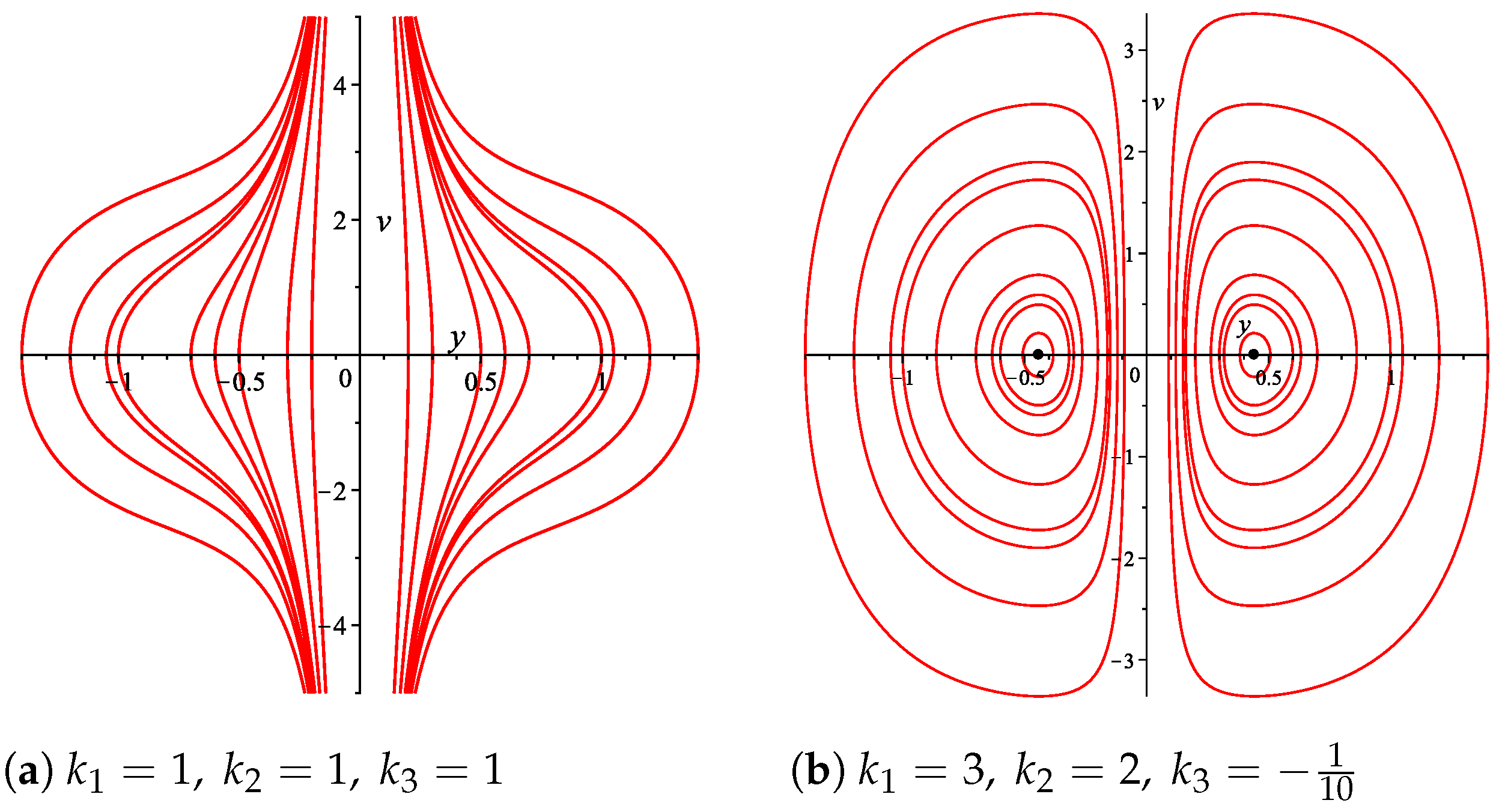
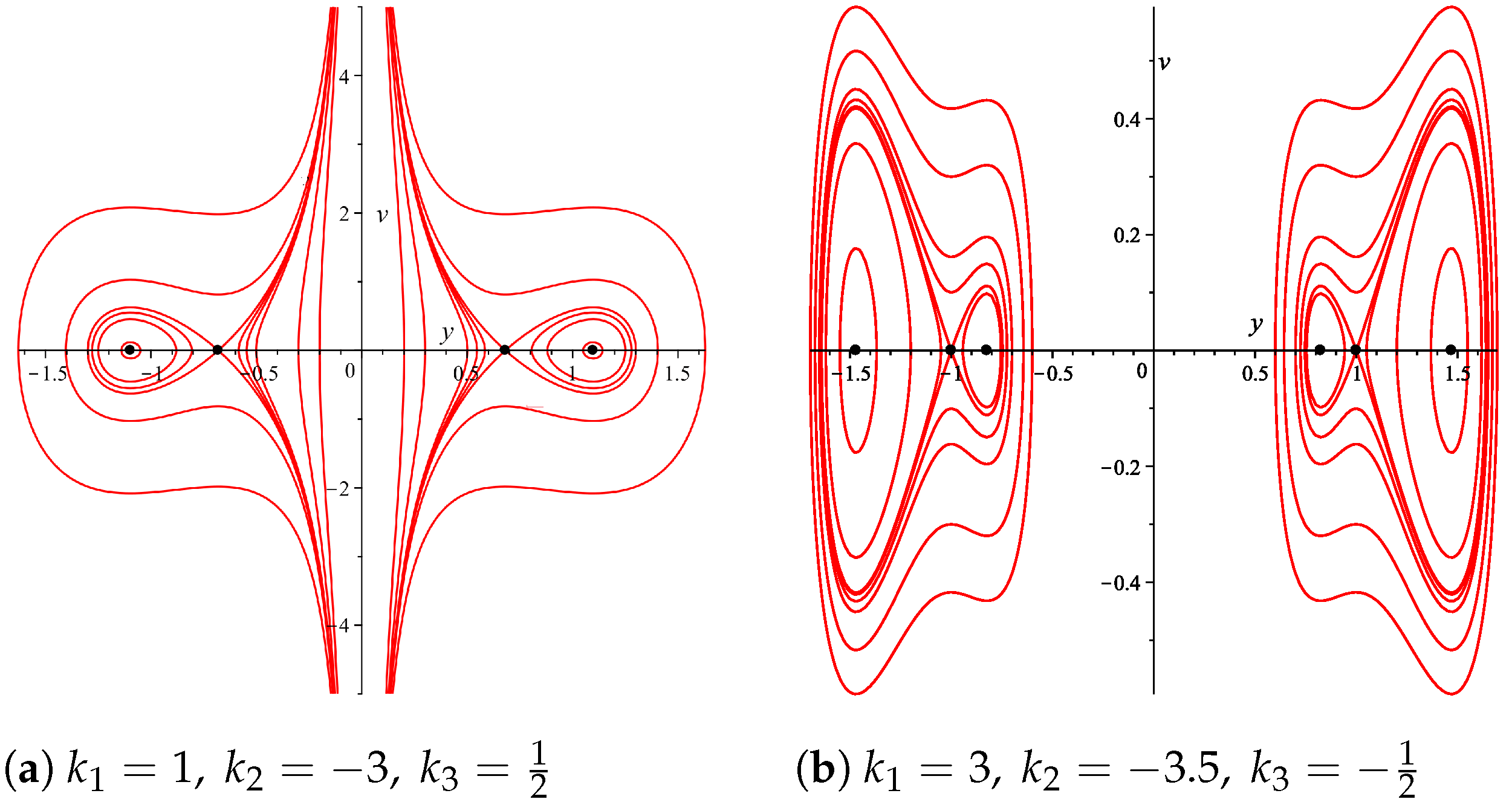
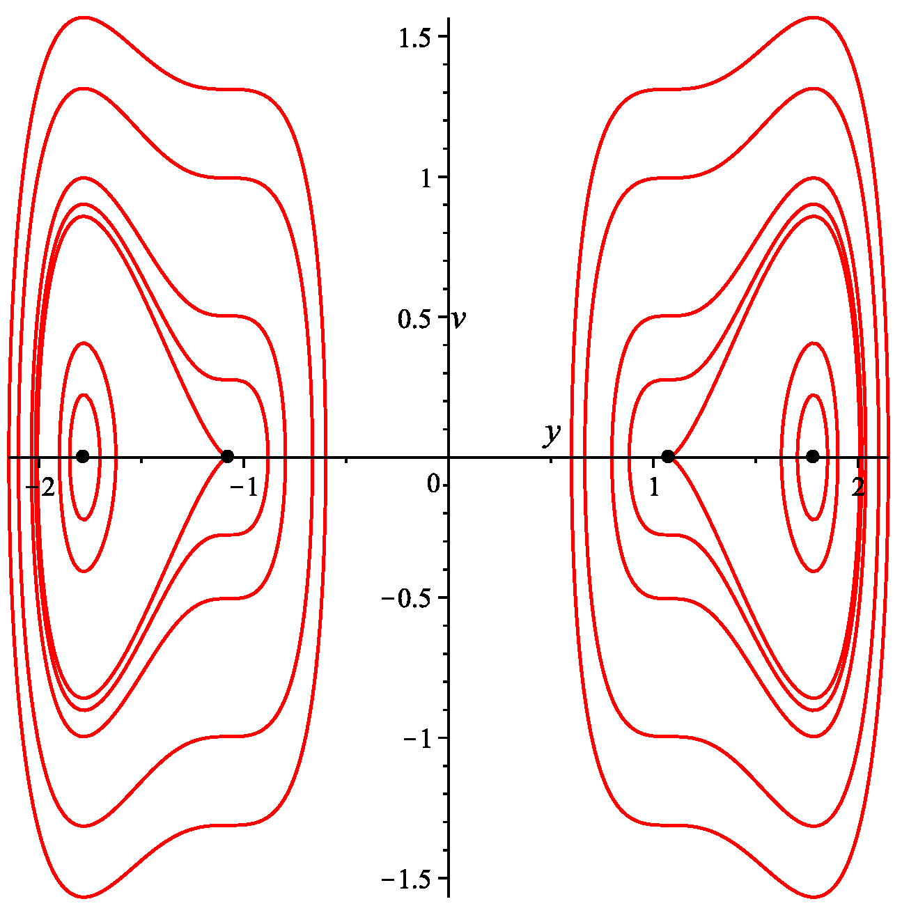
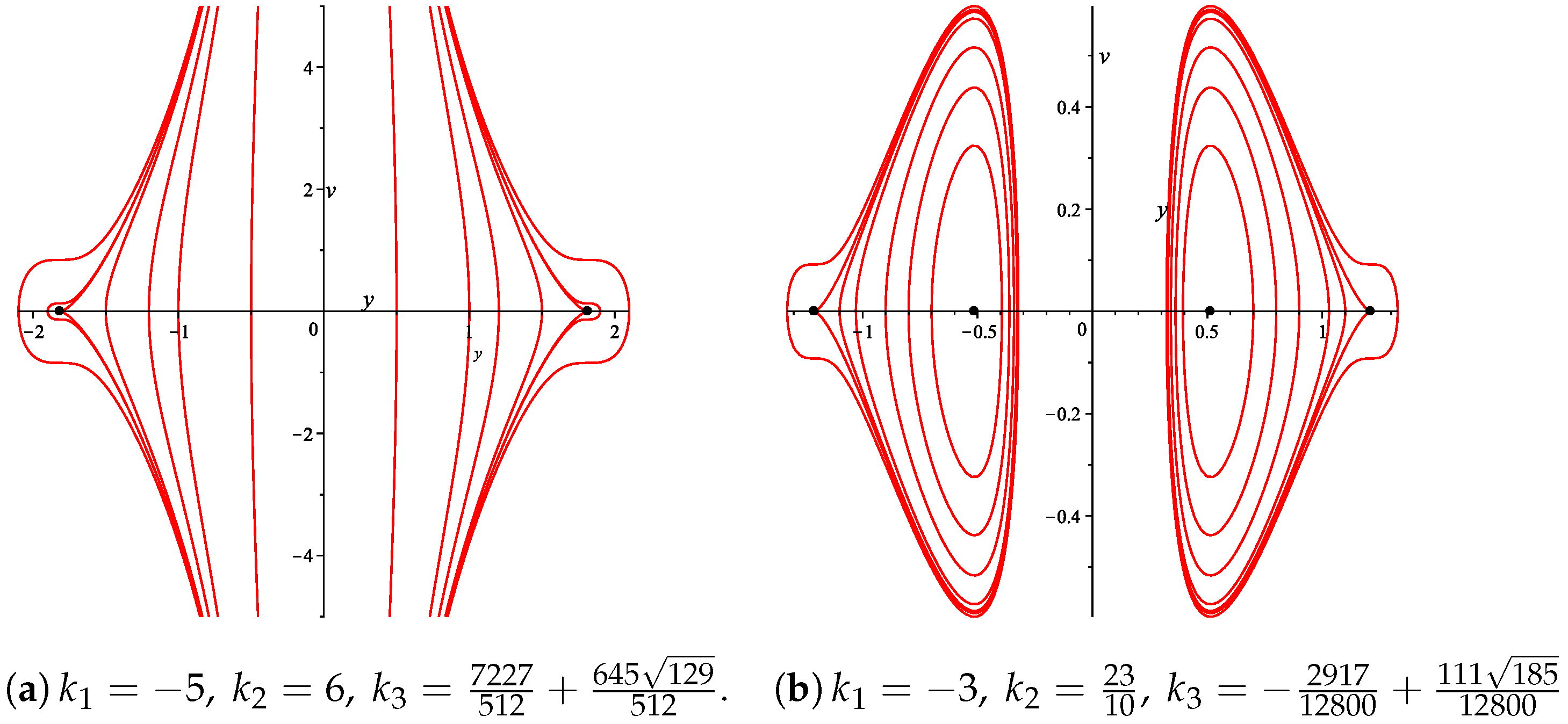
3. Bifurcation of Phase Portraits Corresponding to Equation (6)

In this section, we visualize the results from the previous section by analyzing the stability of equilibrium points of the traveling-wave reduction of the explored equation and study the bifurcations of its phase portraits using the first integral (6) (see [32]). Let us write Equation (6) before integration in its canonical form
y z = v , v z = A y B y 3 C y 5 D y 2 m 1 E y 2 m + 1 F y 2 m + 3 G y 4 m + 1 H y 3 ,
where parameters A, B, C, E, F and H are determined by formulas
A = 4 ω a + α 2 + 2 C 0 α + 6 c C 1 + C 0 2 4 a 2 , B = α + C 0 c 2 a 2 , C = 5 c 2 16 a 2 + b a , D = λ 2 μ C 1 m a 2 m + 1 , E = α + C 0 λ 2 a 2 , F = c 5 λ m + 6 μ m + 2 λ 4 a 2 m + 1 , G = 4 μ μ + λ m 2 + 2 λ 2 m + λ 2 4 a 2 m + 1 2 , H = C 1 2 a 2 .
Introducing into (7) the following transformation
d z = y 3 d ξ
yields the associated regular system
y ξ = y 3 v , v ξ = A y 4 B y 6 C y 8 D y 2 m + 2 E y 2 m + 4 F y 2 m + 6 G y 4 m + 4 H .
Ignoring the orientation, the trajectories of systems (7) and (10) are identical; therefore, systems (7) and (10) are topologically equivalent. Due to their first integrals being the same, they also have the same orbits, with the exception of the straight line y = 0 .
The first integral of the regular system (10) is (6), which is written as follows, taking into account the notations of the current section:
H ( y , v ) = v 2 2 + A y 2 2 + B y 4 4 + C y 6 6 + D y 2 m 2 m + E y 2 m + 2 2 m + 2 + + F y 2 m + 4 2 m + 4 + G y 4 m + 2 4 m + 2 H 2 y 2 .
Let us conduct the analysis of the equilibrium point stability for the regular system (10). All of its equilibrium points are located on the y axis (provided that H 0 ), with the coordinate determined by the following equation
A y 4 + B y 6 + C y 8 + D y 2 m + 2 + E y 2 m + 4 + F y 2 m + 6 + G y 4 m + 4 + H f m ( y ) = 0 .
The stability of an equilibrium point ( y s , 0 ) is determined by the eigenvalues of the following Jacobi matrix
J = 0 y s 3 d f m ( y ) d y ( y s ) 0 ,
where y s solves Equation (12).
One can see that the point ( y s , 0 ) is of the center stability type if f m ( y ) decreases at y s and y s > 0 , it is of the saddle stability type if f m ( y ) increases at y s and y s > 0 (if y s < 0 , then the stability type is reversed), and ( y s , 0 ) is a degenerate point if f m ( y ) has a zero derivative at the equilibrium point and, therefore, a zero eigenvalue, since the eigenvalues of the matrix J are determined by the following formula
λ 1 , 2 = ± y s 3 · d f m d y ( y s ) .
For example, let us explore the case of m = 1 . Equation (12) takes the form
( A + D ) y 4 + ( B + E ) y 6 + ( C + F + G ) y 8 + H f 1 ( y ) = 0 .
Making the change of variables y 2 = w yields
w 4 + k 1 w 3 + k 2 w 2 + k 3 = 0 f 1 ( w ) ( C + F + G ) ,
where
k 1 = B + E C + F + G , k 2 = A + D C + F + G , k 3 = H C + F + G .
The discriminant of Equation (16) is as follows:
D 0 = k 3 27 k 1 4 k 3 + 4 k 1 2 k 2 3 144 k 1 2 k 2 k 3 16 k 2 4 + 128 k 2 2 k 3 256 k 3 2 .
Thus, our explored system for m = 1 can have either zero, two, four or six equilibrium points ( y s , 0 ) = ( ± w s , 0 ) , since Equation (16) can possess at most three positive roots.
Let us introduce the notation
w ± = 3 k 1 ± 9 k 1 2 32 k 2 8 ,
where w ± are the turning points of the function f 1 ( w ) , besides the turning point w 0 = 0 .
Based on the control parameter values, the sign of the discriminant (18) and the values of f 1 ( w ± ) , there exist the following combinations of roots of Equation (16) (in particular, we are interested in the positive ones, due to the nature of the substitution y 2 = w ):
  • k 1 0 , k 2 0 , k 3 > 0 , D 0 > 0 —Equation (16) has no real roots. The system (10) has no equilibria (Figure 1a).
  • k 1 > 0 , k 2 0 , k 3 > 0 , D 0 < 0 —Equation (16) has two real negative roots. The system (10) has no equilibria.
  • k 1 > 0 , k 2 > 0 , k 3 < 0 , D 0 > 0 —Equation (16) has four real roots only one of which is positive. The system (10) has two equilibria (Figure 1b).
  • k 1 0 , k 2 0 , k 3 < 0 , D 0 < 0 —Equation (16) has two real roots, one of which one is positive. The system (10) has two equilibria.
  • k 1 0 , k 2 < 0 , k 3 > 0 , D 0 > 0 —Equation (16) may have four real roots, out of which two are positive, provided that f 1 ( w + ) < 0 and w + R . The system (10) has two equilibria of the center type and two saddle equilibria (Figure 2a)
  • k 1 > 0 , k 2 0 , k 3 > 0 , D 0 < 0 —Equation (16) has two real roots, out of which two are negative. The system (10) has no equilibria.
  • k 1 0 , k 2 0 , k 3 < 0 , D 0 > 0 —an impossible case.
  • k 1 0 , k 2 0 , k 3 < 0 , D 0 < 0 —Equation (16) has two real roots with one of them positive. The system (10) has two equilibria.
  • k 1 0 , k 2 0 , k 3 > 0 , D 0 > 0 —Equation (16) has no real roots. The system (10) has no equilibria.
  • k 1 < 0 , k 2 0 , k 3 > 0 , D 0 < 0 —Equation (16) has two real positive roots. The system (10) has two equilibria of the center type and two saddle equilibria.
  • k 1 < 0 , k 2 > 0 , k 3 < 0 , D 0 > 0 —Equation (16) has four real roots, three of which are positive. The system (10) has four centers and two saddles (Figure 2b).
  • k 1 0 , k 2 0 , k 3 < 0 , D 0 < 0 —Equation (16) has two real roots with one of them positive. The system (10) has two equilibria.
  • k 1 0 , k 2 < 0 , k 3 > 0 , D 0 > 0 —Equation (16) has four real roots with two of them positive if f ( w + ) < 0 and w + R and no real roots otherwise. The system (10) has either two centers and two saddles or no equilibria.
  • k 1 < 0 , k 2 0 , k 3 > 0 , D 0 < 0 —Equation (16) has two real roots with two of them positive if f ( w + ) < 0 and negative otherwise. The system (10) has either two centers and two saddles or no equilibria.
  • k 1 < 0 , k 2 < 0 , k 3 < 0 , D 0 > 0 —an impossible case.
  • k 1 0 , k 2 0 , k 3 < 0 , D 0 < 0 —Equation (16) has two real roots, out of which one is positive. The system (10) has two equilibria.
All the above cases do not include degenerate equilibria, since for d f 1 d y | y s = 0 , we must have D 0 = 0 .
The degenerate cases can show the parameter values at which solitary-wave solutions vanish. For instance, Figure 2b and Figure 3a show how the phase plane may transform from having four solitary waves represented by homoclinic orbits to two solitary waves. Cases where degenerate equilibria exist and D 0 = 0 are as follows:
  • k 3 = 0 . Two zero roots and two roots w 1 , 2 = k 1 ± k 1 2 4 k 2 2 that are real if k 2 < k 1 2 4 .
  • k 3 = 9 k 1 3 + 32 k 1 k 2 9 k 1 2 32 k 2 512 + 27 k 1 4 512 9 k 1 2 k 2 32 + k 2 2 4 and 9 k 1 2 32 k 2 > 0 . At the root w + = 3 k 1 + 9 k 1 2 32 k 2 8 of Equation (16), f 1 ( y ) has a zero derivative; therefore, the equilibrium points y + = ± ( w + , 0 ) are degenerate provided that w + > 0 . There may exist one additional positive root of (16) depending on the parameter values, making it either two equilibria (Figure 4a) or four equilibria for system (10) (Figure 4b).
  • k 3 = 9 k 1 3 32 k 1 k 2 9 k 1 2 32 k 2 512 + 27 k 1 4 512 9 k 1 2 k 2 32 + k 2 2 4 . At the root w = 3 k 1 9 k 1 2 32 k 2 8 of Equation (16), f 1 ( y ) has a zero derivative; therefore, the equilibrium points y = ± ( w , 0 ) are degenerate provided that w > 0 . There also exists one additional positive root of (16), making it four equilibria for system (10) (Figure 3a).
Based on the above analysis of the equilibrium point stability of the system, we can choose suitable parameter values for which solitary or periodic solutions of system (7) exist. Figure 2a,b, Figure 3a and Figure 4b all contain cases for which Equation (7) admits a solitary solution.

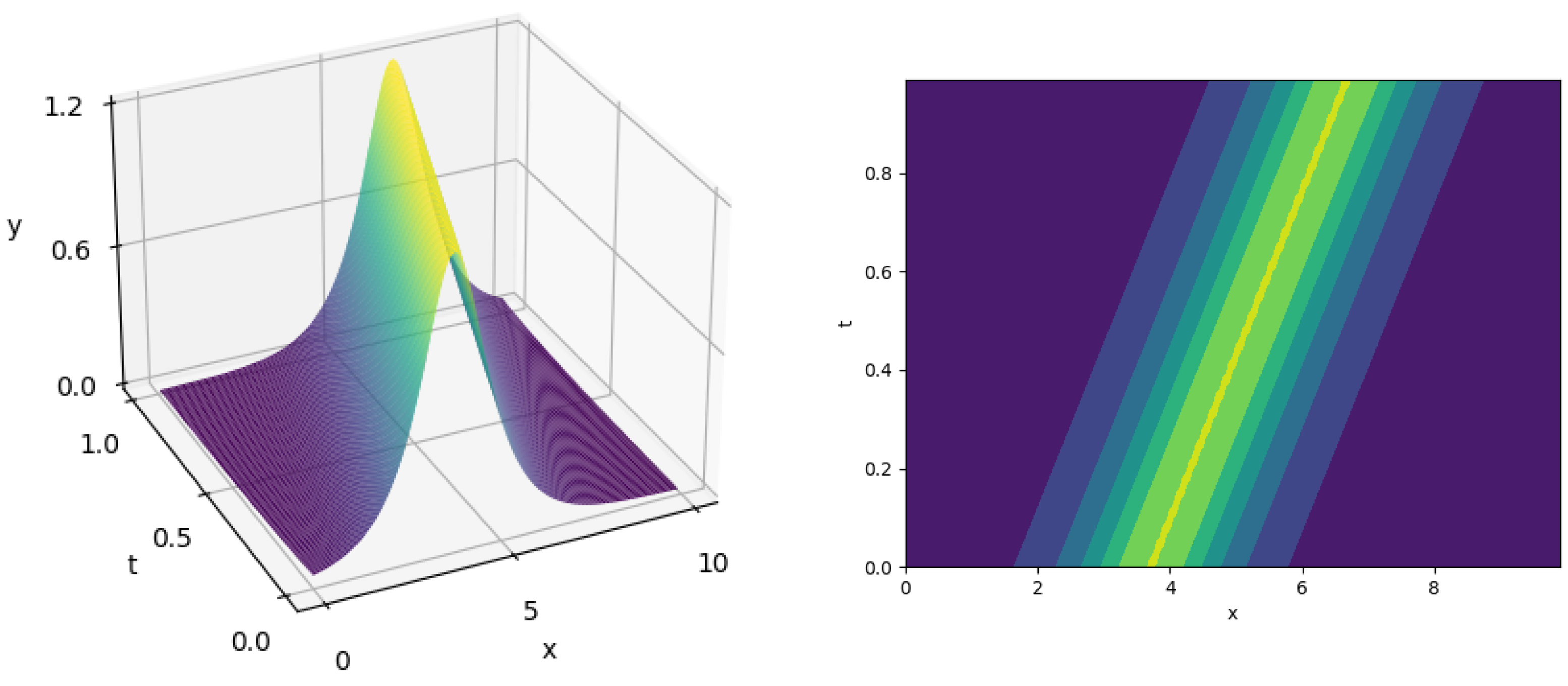
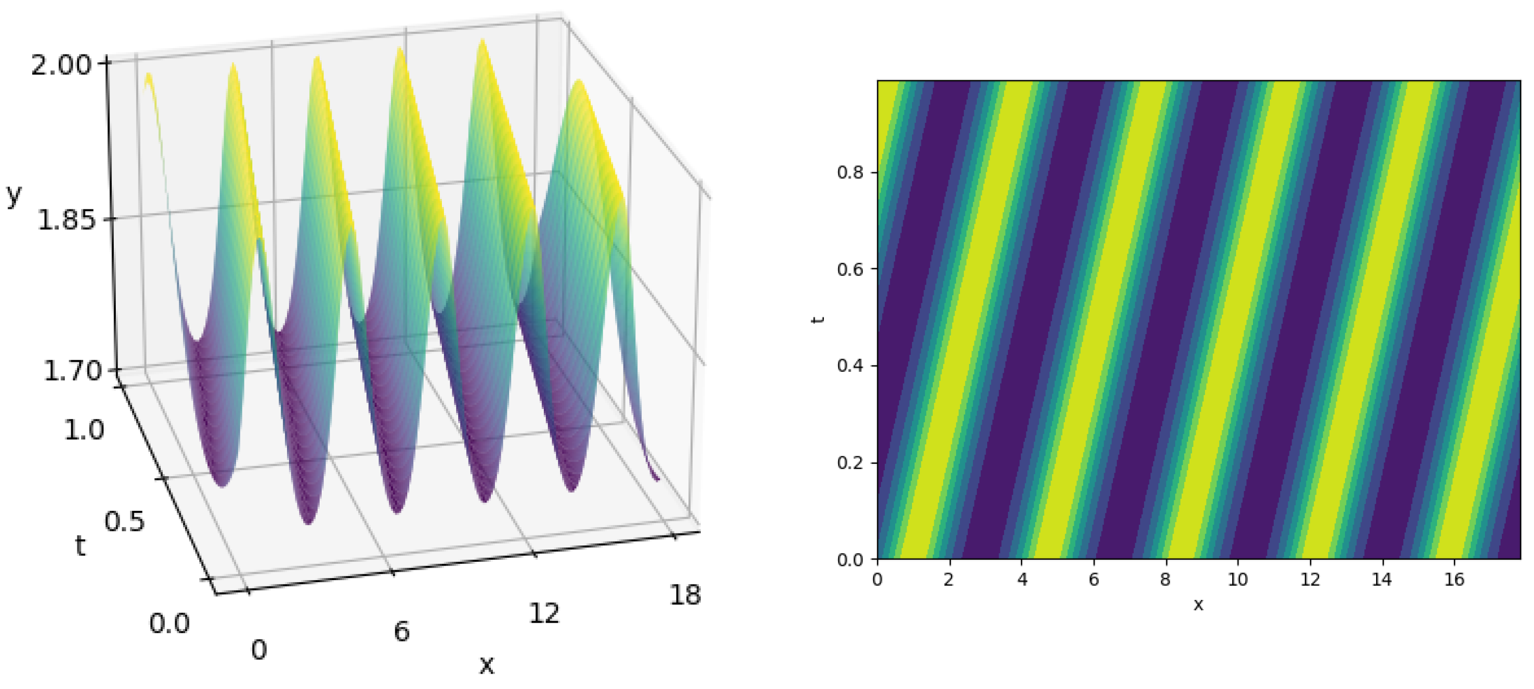
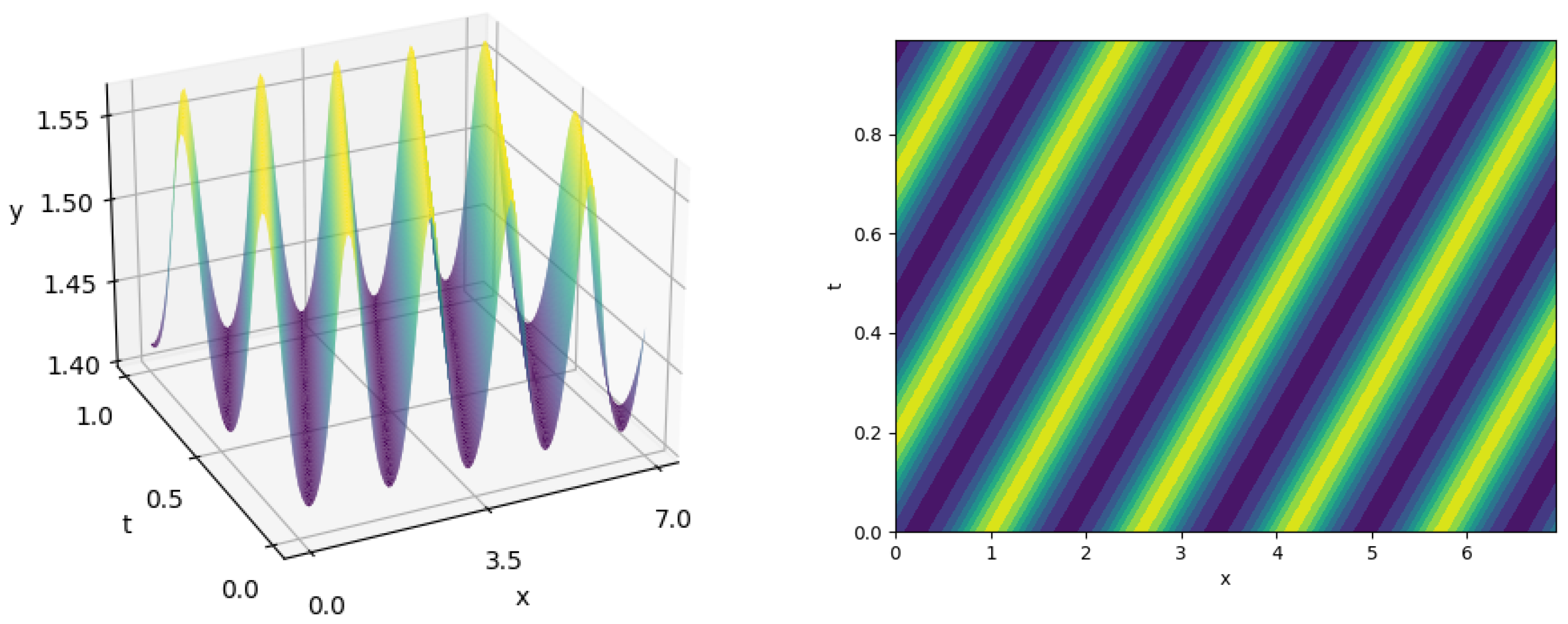
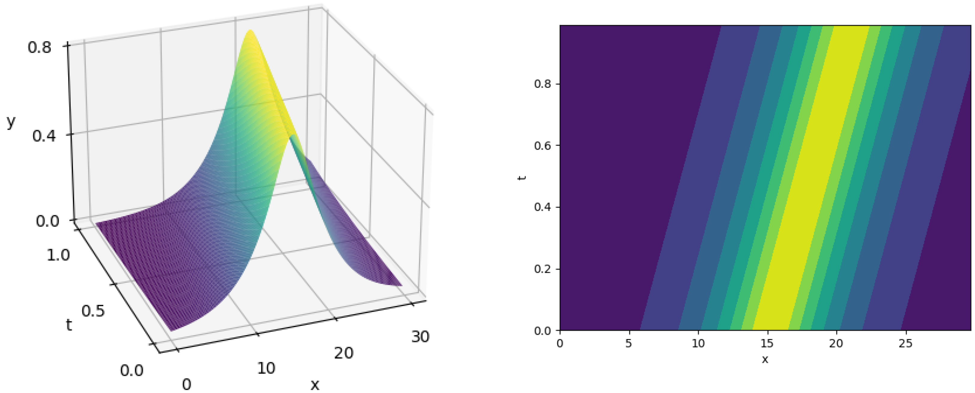
4. Periodic and Solitary Waves of Equation (1) at m = 1

The solution of Equation (6) in the general case cannot be presented in the form of quadratures. However, this integral can be calculated in a number of partial cases. Equation (6) at m = 1 can be written as follows:
a 2 y z 2 + b 6 5 c 2 96 a λ μ 24 a μ 2 24 a + λ 2 32 a + 7 λ c 48 a + c μ 8 a y 6 + + C 0 c 8 a + c α 8 a + λ C 0 8 a + λ α 8 a y 4 + ω 2 + 3 c C 1 4 a + C 0 2 8 a + + C 0 α 4 a + α 2 8 a λ C 1 4 a C 1 μ 2 a y 2 + C 1 2 2 a y 2 C 2 = 0 .
To simplify Equation (20), we introduce a new variable (see [33,34,35])
y ( z ) = V ( z ) ;
we obtain
V z 2 + A 1 V 4 + B 1 V 3 E 1 V 2 8 C 2 a V + 4 C 1 2 a 2 = 0 ,
where A 1 , B 1 and E 1 are determined by formulas
A 1 = 4 b 3 a 5 c 2 12 a 2 μ 2 3 a 2 + λ 2 4 a 2 λ μ 3 a 2 + 7 λ c 6 a 2 + c μ a 2 , B 1 = C 0 c a 2 + c α a 2 + λ C 0 a 2 + λ α a 2 , E 1 = 4 ω a C 0 2 a 2 2 C 0 α a 2 α 2 a 2 + 2 λ C 1 a 2 + 4 μ C 1 a 2 6 c C 1 a 2 .
At C 1 = 0 and C 2 = 0 , the solution of Equation (20) is the solitary wave of the form
V ( z ) = 4 E 1 e E 1 ( z z 0 ) 4 A 1 E 1 + B 1 + e E 1 ( z z 0 ) 2 ,
where z 0 is an arbitrary constant. Solution y ( z ) is expressed by the formula
y 1 ( z ) = 4 E 1 e E 1 ( z z 0 ) 4 A 1 E 1 + B 1 + e E 1 ( z z 0 ) 2 1 / 2 .
The solitary wave for q ( x , t ) can be written as follows:
q 1 ( x , t ) = 4 E 1 e E 1 ( x C 0 t z 0 ) 4 A 1 E 1 + B 1 + e E 1 ( x C 0 t z 0 ) 2 1 / 2 e i ( ψ ( x C 0 t ) ω t ) .
Here, the function ψ ( z ) is found as a result of solving Equation (5)
ψ ( z ) = 2 μ + 3 λ c 2 a A 1 arctan e E 1 ( z z 0 ) + B 1 2 A 1 E 1 + C 0 + α 2 a z .
Solution (25) is illustrated in Figure 5 at z 0 = 3.0 , A 1 = 1.0 , B 1 = 2.0 and E 1 = 5.0 .
The general solution of Equation (20) can be found by taking into account the Jacobi elliptic function. It is well known that the solution of Equation (20) is expressed in terms of elliptic Jacobi or Weierstrass functions. The general solution at C 1 0 and C 2 0 of Equation (20) takes the form
y 2 ( z ) = V 1 ( V 4 V 2 ) sn 2 S 1 ( z z 0 ) , k 1 + V 4 ( V 2 V 1 ) ( V 4 V 2 ) sn 2 S 1 ( z z 0 ) , k 1 + V 2 V 1 1 / 2 ,
provided that the following equation
A 1 V 4 + B 1 V 3 E 1 V 2 8 C 2 a V + 4 C 1 2 a 2 = = A 1 ( V V 1 ) ( V V 2 ) ( V V 3 ) ( V V 4 ) = 0
has four real roots V 1 , V 2 , V 3 and V 4 .
Values S 1 and k 1 are given by formulas
S 1 = 1 2 A 1 ( V 4 V 3 ) ( V 2 V 1 )
and
k 1 = ( V 3 V 1 ) ( V 4 V 2 ) ( V 4 V 3 ) ( V 2 V 1 ) .
The periodic solution q 2 ( x , t ) of Equation (1) at m = 1 is determined by Formula (2), taking into account (28).
Periodic solution (28) is illustrated in Figure 6 at z 0 = 1.0 , A 1 = 1.0 , V 1 = 1.0 , V 2 = 3.0 , V 3 = 2.0 and V 4 = 4.0 .

5. General Solution of Equation (6) at m = 2

Equation (6) at m = 2 takes the form
a 2 y z 2 C 2 + C 1 2 2 a y 2 + 3 c C 1 4 a + ω 2 + α 2 8 a + C 0 α 4 a + C 0 2 8 a y 2 + + C 0 c 8 a + c α 8 a C 1 μ 3 a λ C 1 6 a y 4 + b 6 5 c 2 96 a + λ α 12 a + λ C 0 12 a y 6 + + c λ 8 a + c μ 8 a y 8 + λ 2 72 a 2 λ μ 45 a 2 μ 2 45 a y 10 = 0 .
Let us assume that the following conditions in Equation (32) are satisfied:
C 2 = 0 , μ = λ , C 0 = α 4 λ C 1 3 c .
Substituting a new variable in Equation (32)
y = W ( z ) 1 / 4 ,
yields the following equation
W z 2 + 16 C 1 2 a 2 W + 24 c C 1 a 2 + 16 ω a + 64 9 λ 2 C 1 2 a 2 c 2 W 2 + + 16 b 3 a 5 c 2 3 a 2 32 9 λ 2 C 1 a 2 c W 3 + 4 λ 2 9 a 2 W 4 = 0 .
Equation (35) can be written in the following form
W z 2 + 16 C 1 2 a 2 W R W 2 + N W 3 + 4 λ 2 9 a 2 W 4 = 0 ,
where N and R are determined by formulas
R = 24 c C 1 a 2 + 16 ω a + 64 9 λ 2 C 1 2 a 2 c 2 ,
N = 16 b 3 a 5 c 2 3 a 2 32 9 λ 2 C 1 a 2 c .
The general solution of Equation (36) is also expressed via the elliptic function
W ( z ) = W 3 W 1 ( W 3 W 1 ) sn 2 S 2 ( z z 0 ) , k 2 + W 1 ,
provided that the following equation
16 C 1 2 a 2 R W + N W 2 + 4 λ 2 9 a 2 W 3 = 0
has three real roots W 1 , W 2 and W 3 . The values S 2 and k 2 are determined by formulas
S 2 = λ 3 a ( W 3 W 2 ) W 1
and
k 2 = ( W 3 W 1 ) W 2 ( W 3 W 2 ) W 1 .
The general solution of Equation (32) is expressed at conditions (33) by the formula
y 3 ( z ) = W 3 W 1 ( W 3 W 1 ) sn 2 S 2 ( z z 0 ) , k 2 + W 2 1 / 4 .
Periodic solution (43) is illustrated in Figure 7 at z 0 = 1.0 , a = 1.0 , λ = 3.0 , W 1 = 3.0 , W 2 = 2.0 and W 3 = 4.0 .
At C 1 = 0 , we have the solitary-wave solution of Equation (35) of the form
W ( z ) = 36 R a 2 e R ( z 0 z ) 144 λ 2 R a 2 + 9 N a 2 + e R ( z 0 z ) 2
and the solution of Equation (32) of the form
y 4 ( z ) = 36 R a 2 e R ( z 0 z ) 144 λ 2 R a 2 + 9 N a 2 + e R ( z 0 z ) 2 1 / 4 .
Solution (45) allows us to find the solution of Equation (1) by Formula (2).
Solitary-wave solution (45) is illustrated in Figure 8 at z 0 = 20.0 , a = 2.0 , λ = 4.0 , R = 1.0 and N = 2.0 .

6. Exact Solutions of Equation (1) at an Arbitrary m

There are solitary-wave solutions with additional conditions on the parameters of Equation (6) at an arbitrary value of m. Assuming
C 1 = 0 , C 2 = 0 , C 0 = α , b = 5 16 c 2 a , μ = ( 2 + 5 m ) λ 6 m ,
we have Equation (6) in the form
y z 2 + 5 λ 2 36 a 2 ( 2 m + 1 ) y 4 m + 2 + ω a y 2 = 0 .
Using the new variable
y ( z ) = W ( z ) 1 / 2 m
we obtain the equation
W z 2 M W 2 + N W 4 = 0 ,
where
M = 4 m 2 ω a , N = 5 m 2 λ 2 9 a 2 ( 2 m + 1 ) .
The solution of Equation (49) is the solitary-wave solution of the form
W ( z ) = 4 M e M ( z z 0 ) 4 M N + e 2 M ( z z 0 ) .
The solution of Equation (47) is
y 5 ( z ) = 4 M e M ( z z 0 ) 4 M N + e 2 M ( z z 0 ) 1 / 2 m .
Solitary-wave solution (52) is illustrated in Figure 9 at m = 3 , z 0 = 2.0 , M = 4.0 and N = 3.0 .
Solution (52) gives a solitary wave of Equation (1). We have obtained that there is a solution of the generalized Gerdjikov–Ivanov equation in the form of a solitary wave at an arbitrary value of m.

7. Conservation Laws Corresponding to Equation (1)

Conservation laws are important characteristics of partial differential equations, which are especially useful in practical applications for numerical schemes testing. In this section, we find three conservation laws corresponding to Equation (1). In order to look for these laws, we write Equation (1) as the system of equations of the form (see, for example, [36])
i q t + a q x x + b | q | 4 q + i c q 2 q x = i [ α q x + λ ( | q | 2 m q ) x + μ ( | q | 2 m ) x q ] .
and
i q t + a q x x + b | q | 4 q i c q 2 q x = i [ α q x + λ ( | q | 2 m q ) x + μ ( | q | 2 m ) x q ] .
Firstly, let us find the first conservation law of Equation (53). With this aim, we multiply Equation (53) by q and Equation (54) by q and then add these equations. As a result, we obtain the following equality:
T 1 t + X 1 x = 0 ,
where T 1 and X 1 are as follows:
T 1 = | q | 2 , X 1 = i a ( q q x q q x ) + c 2 | q | 4 α | q | 2 λ ( 2 1 m + 1 ) | q | 2 ( m + 1 ) 2 μ m m + 1 | q | 2 ( m + 1 ) .
In order to obtain the second conservation law, we use a similar approach to the first law. Differentiating Equations (53) and (54) with respect to x, multiplying the first equation by q and the second equation by q, and then adding them yields
t ( q q x q q x ) + X 2 ( 1 ) x + 2 c | q | 2 ( q q x x q q x x ) = = 2 ( λ + μ ) [ | q | 2 m ( q q x x q q x x ) ] ,
where X 2 ( 1 ) is as follows:
X 2 ( 1 ) = i a ( q q x x + q q x x 2 | q x | 2 ) 4 3 i b | q | 6 + c | q | 2 ( q q x q q x ) α ( q q x q q x ) λ ( ( | q | 2 m q ) x q ( | q | 2 m q ) x q + + 2 | q | 2 m ( q q x q q x ) ) 2 μ | q | 2 m ( q q x q q x ) .
Multiplying Equation (53) by q | q | 2 k and adding Equation (54) multiplied by q | q | 2 k , where k N , yields
i k + 1 t ( | q | 2 k + 2 ) + X 2 ( 2 ) x + a | q | 2 k ( q q x x q q x x ) = 0 .
where X 2 ( 2 ) is as follows:
X 2 ( 2 ) = i c k + 2 | q | 2 ( k + 2 ) i α k + 1 | q | 2 ( k + 1 ) i λ 2 m + 1 k + m + 1 | q | 2 ( k + m + 1 ) 2 i μ m k + m + 1 | q | 2 ( k + m + 1 ) .
Adding Equation (57) and Equation (59) at k = 1 and Equation (59) at k = m , we have the second conservation law of the form
T 2 t + X 2 x = 0 ,
where T 2 and X 2 are as follows:
T 2 = a ( q q x q q x ) + i c | q | 4 2 i ( λ + μ ) m + 1 | q | 2 m + 2 , X 2 = a X 2 ( 1 ) + 2 c X 2 ( 2 ) | k = 1 2 ( λ + μ ) X 2 ( 2 ) | k = m .
In order to obtain the third conservation law, we apply a similar approach. With this aim, we multiply Equation (53) by q t and Equation (54) by q t and then add these equations. As a result, we obtain the following equality:
a ( q x x q t + q x x q t ) + b | q | 4 ( q q t + q q t ) + i c ( q 2 q x q t q 2 q x q t ) = = i [ α ( q x q t q x q t ) + λ ( ( | q | 2 m q ) x q t ( | q | 2 m q ) x q t ) + + μ ( | q | 2 m ) x ( q q t q q t ) ] .
In the case μ = λ ,
a ( q x x q t + q x x q t ) + b | q | 4 ( q q t + q q t ) + i c ( q 2 q x q t q 2 q x q t ) = = i [ α ( q x q t q x q t ) + λ | q | 2 m ( q x q t q x q t ) ] .
At the next step, we obtain
x ( a ( q x q t + q x q t ) ) t ( a | q x | 2 ) + t ( b | q | 6 3 ) + x ( i c 2 ( q 2 q q t q 2 q q t ) ) + t ( i c 2 ( q 2 q q x q 2 q q x ) ) + i c | q | 2 ( q q x t q q x t ) = x ( i α 2 ( q q t q q t ) ) + t ( i α 2 ( q x q q x q ) + + x ( i λ 2 ( m + 1 ) 2 ( q m + 1 ( ( q ) m + 1 ) t ( q ) m + 1 ( q m + 1 ) t ) ) + + t ( i λ 2 ( m + 1 ) 2 ( ( q m + 1 ) x ( q ) m + 1 ( ( q ) m + 1 ) x q m + 1 ) ) .
As a result, we obtain the following equality:
T 3 ( 1 ) t + i c | q | 2 ( q q x t q q x t ) + X 3 ( 1 ) x = 0 ,
where T 3 ( 1 ) and X 3 ( 1 ) are as follows:
T 3 ( 1 ) = b | q | 6 3 a | q x | 2 i c | q | 2 2 ( q q x q q x ) i α 2 ( q q x q q x ) i λ | q | 2 m 2 ( m + 1 ) ( q q x q q x ) , X 3 ( 1 ) = a ( q x q t + q x q t ) + i c | q | 2 2 ( q q t q q t ) i α 2 ( q q t q q t ) i λ | q | 2 m 2 ( m + 1 ) ( q q t q q t ) .
Differentiating Equations (53) and (54) with respect to x and then multiplying the first equation by c | q | 2 q and the second equation by c | q | 2 q , we have
i c | q | 2 ( q q x t q q x t ) + a c | q | 2 ( q q 3 , x + q q 3 , x ) + 5 4 b c x ( | q | 8 ) + + i c 2 | q | 4 x ( q q x q q x ) = i α c | q | 2 x ( q q x q q x ) + + i λ c | q | 2 ( m + 1 ) m + 1 x ( q q x q q x ) + i λ c m m + 1 x ( | q | 2 ( m + 1 ) ( q q x q q x ) ) .
Further, we take into account the following equality:
a c | q | 2 ( q q 3 , x + q q 3 , x ) = a c | q | 2 x ( q q x x + q q x x q x q x ) = = a c | q | 2 x ( q q x x + q q x x + 2 q x q x 3 q x q x ) = a c | q | 2 3 x 3 ( | q | 2 ) 3 a c | q | 2 x ( q x q x ) = x ( a c | q | 2 ( | q | 2 ) x x ) a c ( | q | 2 ) x ( | q | 2 ) x x 3 a c | q | 2 x ( q x q x ) = x ( a c | q | 2 ( | q | 2 ) x x ) x ( a c 2 ( ( | q | 2 ) x ) 2 ) 3 a c | q | 2 x ( q x q x ) .
We transform Expression (68), using Equation (59):
i c | q | 2 ( q q x t q q x t ) = x ( a c | q | 2 ( | q | 2 ) x x ) + x ( a c 2 ( ( | q | 2 ) x ) 2 ) + + 3 a c | q | 2 x ( q x q x ) x ( 5 4 b c | q | 8 ) + t ( c 2 3 a | q | 6 ) x ( i c 2 a X 2 ( 2 ) ) | k = 2 + + t ( α c 2 a | q | 4 ) x ( i α c a X 2 ( 2 ) ) | k = 1 + t ( λ c a ( m + 1 ) ( m + 2 ) | q | 2 ( m + 2 ) ) x ( i λ c a ( m + 1 ) X 2 ( 2 ) ) | k = m + 1 + x ( i λ c m m + 1 | q | 2 ( m + 1 ) ( q q x q q x ) ) .
Multiplying Equation (53) by 3 c | q | 2 q x , Equation (54) by 3 c | q | 2 q x , and then adding the resulting expressions yields
3 i c | q | 2 ( q t q x q x q t ) + 3 a c | q | 2 x ( q x q x ) + x ( 3 4 b c | q | 8 ) + + 3 2 i c 2 | q | 4 x ( q q x q q x ) x ( 3 i c 2 2 | q | 4 ( q q x q q x ) ) = 0
We transform Expression (71) using Equation (59):
3 a c | q | 2 x ( q x q x ) = t ( 3 4 i c | q | 2 ( q q x q q x ) ) + x ( 3 4 i c | q | 2 ( q q t q q t ) ) x ( 3 4 b c | q | 8 ) t ( c 2 2 a | q | 6 ) + x ( 3 i c 2 2 a X 2 ( 2 ) ) | k = 2 + + x ( 3 i c 2 2 | q | 4 ( q q x q q x ) )
Substituting Equation (72) into Equation (70) yields
i c | q | 2 ( q q x t q q x t ) = T 3 ( 2 ) t + X 3 ( 2 ) x ,
where T 3 ( 2 ) and X 3 ( 2 ) are as follows:
T 3 ( 2 ) = c 2 6 a | q | 6 + α c 2 a | q | 4 + λ c a ( m + 1 ) ( m + 2 ) | q | 2 ( m + 2 ) + + 3 4 i c | q | 2 ( q q x q q x ) , X 3 ( 2 ) = a c | q | 2 ( | q | 2 ) x x + a c 2 ( ( | q | 2 ) x ) 2 2 b c | q | 8 + 1 2 i c 2 a X 2 ( 2 ) | k = 2 i α c a X 2 ( 2 ) | k = 1 i λ c a ( m + 1 ) X 2 ( 2 ) | k = m + 1 + i λ c m m + 1 | q | 2 ( m + 1 ) ( q q x q q x ) + + 3 4 i c | q | 2 ( q q t q q t ) + 3 i c 2 2 | q | 4 ( q q x q q x ) .
Substituting Equation (73) and using Equation (66), we obtain
T 3 t + X 3 x = 0 ,
where T 3 ( 2 ) and X 3 ( 2 ) are as follows:
T 3 = c 2 6 a | q | 6 + α c 2 a | q | 4 + λ c a ( m + 1 ) ( m + 2 ) | q | 2 ( m + 2 ) + + 1 4 i c | q | 2 ( q q x q q x ) + b | q | 6 3 a | q x | 2 i α 2 ( q q x q q x ) i λ | q | 2 m 2 ( m + 1 ) ( q q x q q x ) , X 3 = X 3 ( 1 ) + X 3 ( 2 ) .

8. Conservation Quantities

Let us consider Solution (26) and find conservation quantities for it.
Let us consider the following integrals:
L 1 = y 1 2 d x = 4 E 1 e E 1 ( x C 0 t z 0 ) 4 A 1 E 1 + B 1 + e E 1 ( x C 0 t z 0 ) 2 d x = = 2 A 1 π 2 arctan γ ,
L 2 = y 1 4 d x = 4 E 1 e E 1 ( x C 0 t z 0 ) 4 A 1 E 1 + B 1 + e E 1 ( x C 0 t z 0 ) 2 2 d x = = E 1 A 1 π γ + 2 γ arctan γ + 2 ,
L 3 = y 1 6 d x = 4 E 1 e E 1 ( x C 0 t z 0 ) 4 A 1 E 1 + B 1 + e E 1 ( x C 0 t z 0 ) 2 3 d x = = E 1 2 A 1 A 1 ( 2 ( 3 γ 2 + 1 ) arctan γ + 3 γ ( π γ 2 ) + π ) ,
L = y 1 x 2 d x = E 1 2 e E 1 ( x C 0 t z 0 ) 4 A 1 E 1 + B 1 + e E 1 ( x C 0 t z 0 ) 2 ( 1 2 ( B 1 e E 1 ( x C 0 t z 0 ) + e 2 E 1 ( x C 0 t z 0 ) ) 4 A 1 E 1 + B 1 + e E 1 ( x C 0 t z 0 ) 2 ) 2 d x = = 1 32 A 1 A 1 ( 2 ( γ 2 + 1 ) arctan γ + γ ( π γ 2 ) + π ) ,
where γ = B 1 2 A 1 E 1 .
The density T 1 gives the conservative quantity for the first solution (26) of the form
I 1 ( 1 ) = Re ( T 1 ) d x = | q 1 | 2 d x = y 1 2 d x = L 1 .
The density T 2 gives the conservative quantity for the first solution (26) of the form
I 2 ( 1 ) = Im ( T 2 ) d x = = ( i a ( q 1 q 1 x q 1 q 1 x ) + c | q 1 | 4 ( λ + μ ) | q 1 | 4 ) d x = = 2 a y 1 2 ψ x d x + ( c λ μ ) y 1 4 d x = ( C 0 + α ) y 1 2 d x + + c + λ 2 y 1 4 d x = ( C 0 + α ) L 1 + c + λ 2 L 2 ,
where expression (5) is taken into account.
The density T 3 gives the conservative quantity for the first solution (26)
I 3 ( 1 ) = Re ( a T 3 ) d x = ( c 2 6 | q 1 | 6 + α c 2 | q 1 | 4 + λ c 6 | q 1 | 6 + + i a c 4 | q 1 | 2 ( q 1 q 1 x q 1 q 1 x ) + b a | q 1 | 6 3 a 2 | q 1 x | 2 i α a 2 ( q 1 q 1 x q 1 q 1 x ) i λ a | q 1 | 2 4 ( q 1 q 1 x q 1 q 1 x ) ) d x = α 2 C 0 2 4 y 1 2 d x + ( α ( λ + c ) 4 C 0 ( λ + μ ) 2 ) y 1 4 d x + ( λ c 24 + b a 3 3 λ 2 16 μ λ 2 μ 2 4 5 c 2 48 ) y 1 6 d x a 2 y 1 x 2 d x = α 2 C 0 2 4 L 1 + ( α ( λ + c ) 4 C 0 ( λ + μ ) 2 ) L 2 + λ c 24 + b a 3 3 λ 2 16 μ λ 2 μ 2 4 5 c 2 48 L 3 a 2 L ,
where expression (5) is taken into account.
Let us consider solution (52) and find the conservation quantities for it. Let us consider the following integral
Ω k = ( y 5 ) 2 k d x = 4 M e M ( ( x C 0 t ) z 0 ) 4 M N + e 2 M ( ( x C 0 t ) z 0 ) k m d x = | k m = p | = ( 4 M N ) p N p M 0 φ p 1 ( 1 + φ 2 ) p d φ = ( M ) p 1 ( N ) p π Γ ( p 2 ) Γ ( p + 1 2 ) .
Ω = ( y 5 x ) 2 d x = = M 4 m 2 ( 4 M e M ( ( x C 0 t ) z 0 ) ) 1 m ( 4 M N e 2 M ( ( x C 0 t ) z 0 ) ) 2 ( 4 M N + e 2 M ( ( x C 0 t ) z 0 ) ) 1 m + 2 d x = = M 8 m 3 ( 4 M N ) 1 m Γ 2 ( 1 2 m ) Γ ( 1 m + 2 ) .
The density T 1 gives the conservative quantity for solution (52) of the form
I 1 ( 2 ) = Re ( T 1 ) d x = | q 5 | 2 d x = ( y 5 ) 2 d x = Ω 1 .
The density T 2 gives the conservative quantity for solution (52)
I 2 ( 2 ) = Im ( T 2 ) d x = ( i a ( q 5 q 5 x q q x ) + c | q | 4 2 ( λ + μ ) m + 1 | q | 2 m + 2 ) d x = 2 a y 2 ψ x d x + c y 4 d x λ ( m 2 ) 3 m ( m + 1 ) y 2 ( m + 1 ) d x = λ ( m 2 + 2 ) 3 ( m 2 + m ) y 2 ( m + 1 ) d x + + c 2 y 4 d x = λ ( m 2 + 2 ) 3 ( m 2 + m ) Ω m + 1 + c 2 Ω 2 .
From the condition (46), we receive μ = 2 + 5 m 6 m λ , and for T 3 , there exists a restriction μ = λ . Thus, for T 3 , we have m = 2 .
Density T 3 provides the conservative quantity for solution (52) of the form
I 3 ( 2 ) = Re ( a T 3 ) d x = ( c 2 6 | q | 6 + α c 2 | q | 4 a 2 | q x | 2 + + λ c 12 | q | 8 + 1 4 i c a | q | 2 ( q q x q q x ) + 5 c 2 | q | 6 48 i α a 2 ( q q x q q x ) i λ a | q | 4 6 ( q q x q q x ) ) d x = α c 4 y 4 d x + + λ α 6 y 6 d x + λ 2 36 y 10 d x a 2 y x 2 d x = = α c 4 Ω 2 + λ α 6 Ω 3 + λ 2 36 Ω 5 a 2 Ω .
The conservative quantities I 1 , I 2 and I 3 correspond to the power, impulse and energy of the solitary wave, respectively.

9. Conclusions

In this paper, we have considered the generalized Gerdjikov–Ivanov Equation (1) in the case of arbitrary value m. Equation (1) does not pass the Painlevé test and the Cauchy problem cannot be solved for this equation by the inverse scattering transform. Therefore, we have studied this equation using the traveling wave reduction. We have found the first integral of the nonlinear ordinary differential equation and have presented the classification of the phase portraits corresponding to that equation. Taking into account the classification results, we have obtained the periodic- and solitary-wave solutions of the differential equation at various values m. We have constructed the conservation laws corresponding to Equation (1) by means of direct calculations and have calculated its conserved quantities. The three integrals of motion obtained correspond to the conservation of the power, the momentum and the energy of the optical soliton. These obtained theoretical results can be useful for practical applications as they are helpful in testing whether numerical schemes for partial differential equations are conservative.

Author Contributions

N.A.K.: Conceptualization, Supervision, Idea, Calculations—Section 2, Section 4, Section 5 and Section 6, Writing—Draft. D.R.N.: Checking, Calculations—Section 7 and Section 8. S.F.L.: Writing—Editing, Calculations—Section 4. All authors have read and agreed to the published version of the manuscript.

Funding

This research was supported by the Russian Science Foundation, grant no. 23-41-00070, https://rscf.ru/en/project/23-41-00070/.

Data Availability Statement

Data is contained within the article.

Conflicts of Interest

The authors declare no conflict of interest.

References

  1. Gerdjikov, V.S.; Ivanov, M.I. Expansions over the squared solutions and inhomgeneous nonlinear Schrodinger equation. Inverse Probl. 1992, 8, 831–847. [Google Scholar] [CrossRef]
  2. Zahran, E.H.M.; Bekir, A. New unexpected explicit optical soliton solutions to the perturbed Gerdjikov-Ivanov equation. J. Opt. 2023, 52, 1142–1147. [Google Scholar] [CrossRef]
  3. Farahat, S.E.; Shazly, E.E.; El-Kalla, I.L.; Kader, A.A. Bright, dark and kink exact soliton solutions for perturbed Gerdjikov-Ivanov equation with full nonlinearity. Optik 2023, 277, 170688. [Google Scholar] [CrossRef]
  4. Onder, I.L.; Secer, A.; Ozisik, M.; Bayram, M. Investigation of optical soliton solutions for the perturbed Gerdjikov-Ivanov equation with full-nonlinearity. Heliyon 2023, 9, 2. [Google Scholar] [CrossRef] [PubMed]
  5. Ali, K.K.; Tarla, S.; Sulaiman, T.A.; Yilmazer, R. Optical solitons to the Perturbed Gerdjikov-Ivanov equation with quantic nonlinearity. Opt. Quant. Electron. 2023, 55, 2. [Google Scholar] [CrossRef]
  6. Tang, M.Y. Exact chirped solutions of the perturbed Gerdjikov-Ivanov equation with spatio-temporal dispersion. Zeitschrift für Naturforschung A 2023, 78, 8. [Google Scholar] [CrossRef]
  7. Younis, M.; Bilal, M.; Rehman, S.U.; Seadawy, A.R.; Rizvi, S.T.R. Perturbed optical solitons with conformable time-space fractional Gerdjikov-Ivanov equation. Math. Sci. 2022, 16, 431–443. [Google Scholar] [CrossRef]
  8. Yang, D. New solitons and bifurcations for the generalized Gerdjikov-Ivanov equation in nonlinear fiber optics. Optik 2022, 264, 169394. [Google Scholar] [CrossRef]
  9. Yidirim, Y.; Biswas, A.; Alshehri, H.M.; Belic, M.R. Cubic-quartic optical soliton perturbation with Gerdjikov-Ivanov equation by sine-Gordon equation approach. Optoelectron. Adv. Mat. 2022, 16, 236–242. [Google Scholar]
  10. Al-Kalbani, K.K.; Al-Ghafri, K.S.; Krishnan, E.V.; Biswas, A. Solitons and modulation instability of the perturbed Gerdjikov-Ivanov equation with spatio-temporal dispersion. Chaos Soliton Fract. 2021, 153, 111523. [Google Scholar] [CrossRef]
  11. Lu, P.H.; Wang, Y.Y.; Dai, C.Q. Abundant fractional soliton solutions of a space-time fractional perturbed Gerdjikov-Ivanov equation by a fractional mapping method. Chin. J. Phys. 2021, 74, 96–105. [Google Scholar] [CrossRef]
  12. Xiao, X.; Yin, Z. Exact single travelling wave solutions to the fractional perturbed Gerdjikov-Ivanov equation in nonlinear optics. Mod. Phys. Lett. B 2021, 35, 22. [Google Scholar] [CrossRef]
  13. Muniyappan, A.; Monisha, P.; Nivetha, V. Generation of wing-shaped dark soliton for perturbed Gerdjikov-Ivanov equation in optical fibre. Optik 2021, 230, 166328. [Google Scholar] [CrossRef]
  14. Kudryashov, N.A. Traveling wave solutions of the generalized Gerdjikov-Ivanov equation. Optik 2020, 219, 165193. [Google Scholar] [CrossRef]
  15. Li, C.; Li, G.; Chen, L. Fractional optical solitons of the space-time perturbed fractional Gerdjikov-Ivanov equation. Optik 2020, 224, 165638. [Google Scholar] [CrossRef]
  16. Hosseini, K.; Mirzazadeh, M.; Ilie, M.; Radmehr, S. Dynamics of optical solitons in the perturbed Gerdjikov-Ivanov equation. Optik 2020, 206, 164350. [Google Scholar] [CrossRef]
  17. Guo, L.; Zhang, Y.; Xu, S.; Wu, Z.; He, J. The higher order rogue wave solutions of the Gerdjikov-Ivanov equation. Phys. Scr. 2014, 89, 035501. [Google Scholar]
  18. Zhang, J.B.; Gongye, Y.Y.; Chen, S.T. Soliton solutions to the coupled Gerdjikov-Ivanov equation with rogue-wave-like phenomena. Chin. Phys. Lett. 2017, 34, 090201. [Google Scholar] [CrossRef]
  19. He, B.; Meng, Q. Bifurcations and new exact travelling wave solutions for the Ggerdjikov-Ivanov equation. Commun. Nonlinear. Sci. 2010, 15, 1783–1790. [Google Scholar] [CrossRef]
  20. Biswas, A.; Yildirim, Y.; Yaşar, E.; Babatin, M. Conservation laws for Gerdjikov-Ivanov equation in nonlinear fiber optics and pcf. Optik 2017, 148, 209–214. [Google Scholar] [CrossRef]
  21. Biswas, A.; Ekici, M.L.; Sonmezoglu, A.; Triki, H.; Alshomrani, A.S.; Zhou, Q.; Moshokoa, S.P.; Belic, M. Optical solitons for Gerdjikov-Ivanov model by extended trial equation scheme. Optik 2018, 157, 1241–1248. [Google Scholar] [CrossRef]
  22. Ding, C.C.; Gao, Y.T.; Li, L.Q. Breathers and rogue waves on the periodic background for the Gerdjikov-Ivanov equation for the alfvén waves in an astrophysical plasma. Chaos Soliton Fract. 2019, 120, 259–265. [Google Scholar] [CrossRef]
  23. Biswas, A.; Yildirim, Y.; Yasar, E.; Triki, H.; Alshomrani, A.S.; Ullah, M.Z.; Zhou, Q.; Moshokoa, S.P.; Belic, M. Optical soliton perturbation with full nonlinearity for Gerdjikov-Ivanov equation by trial equation method. Optik 2018, 157, 1214–1218. [Google Scholar] [CrossRef]
  24. Biswas, A.; Yildirim, Y.; Yasar, E.; Triki, H.; Alshomrani, A.S.; Ullah, M.Z.; Zhou, Q.; Moshokoa, S.P.; Belic, M. Optical soliton perturbation with Gerdjikov-Ivanov equation by modified simple equation method. Optik 2018, 157, 1235–1240. [Google Scholar] [CrossRef]
  25. Arshed, S.; Biswas, A.; Abdelaty, M.; Zhou, Q.; Moshokoa, S.P.; Belic, M. Optical soliton perturbation for Gerdjikov-Ivanov equation by extended trial equation method. Optik 2018, 158, 747–752. [Google Scholar]
  26. Arshed, S.; Biswas, A.; Abdelaty, M.; Zhou, Q.; Moshokoa, S.P.; Belic, M. Optical soliton perturbation for Gerdjikov-Ivanov equation via two analytical techniques. Chin. J. Phys. 2018, 56, 2879–2886. [Google Scholar] [CrossRef]
  27. Arshed, S. Two reliable techniques for the soliton solutions of perturbed Gerdjikov-Ivanov equation. Optik 2018, 164, 93–99. [Google Scholar] [CrossRef]
  28. Yildirim, Y. Optical solitons to Gerdjikov-Ivanov equation in birefringent fibers with trial equation integration architecture. Optik 2019, 182, 349–355. [Google Scholar] [CrossRef]
  29. Yildirim, Y. Optical solitons of Gerdjikov-Ivanov equation in birefringent fibers with modified simple equation scheme. Optik 2019, 182, 424–432. [Google Scholar] [CrossRef]
  30. Yildirim, Y. Optical solitons of Gerdjikov-Ivanov equation with four-wave mixing terms in birefringent fibers using trial equation scheme. Optik 2019, 182, 1163–1169. [Google Scholar] [CrossRef]
  31. Ismael, H.F.; Baskonus, H.M.; Bulut, H.; Gao, W. Instability modulation and novel optical soliton solutions to the Gerdjikov-Ivanov equation with M-fractional. Opt. Quantum Electron. 2023, 55, 303. [Google Scholar] [CrossRef]
  32. Kudryashov, N.A.; Lavrova, S.F. Painlevé Test, Phase Plane Analysis and Analytical Solutions of the Chavy–Waddy–Kolokolnikov Model for the Description of Bacterial Colonies. Mathematics 2023, 11, 3203. [Google Scholar] [CrossRef]
  33. Kudryashov, N.A. A generalized model for description of propagation pulses in optical fiber. Optik 2019, 189, 42–52. [Google Scholar] [CrossRef]
  34. Kudryashov, N.A. Implicit solitary waves for one of the generalized nonlinear Schrödinger equations. Mathematics 2021, 9, 3024. [Google Scholar] [CrossRef]
  35. Kudryashov, N.A. Method for finding highly dispersive optical solitons of nonlinear differential equations. Optik 2020, 206, 163550. [Google Scholar] [CrossRef]
  36. Kudryashov, N.A.; Nifontov, D.R. Conservation laws and Hamiltonians of the mathematical model with unrestricted dispersion and polynomial nonlinearity. Chaos Solitons Fract. 2023, 175, 114076. [Google Scholar] [CrossRef]
Figure 1. Phase portraits of system (7) at various parameter values, where parameters k 1 , k 2 and k 3 are determined by (17).
Mathematics 11 04760 g001
Figure 2. Phase portraits of system (7) at various parameter values, where parameters k 1 , k 2 and k 3 are determined by (17).
Mathematics 11 04760 g002
Figure 3. Phase portraits of system (7) at k 1 = 5 , k 2 = 6 , k 3 = 117 512 165 33 512 , where parameters k 1 , k 2 and k 3 are determined by (17).
Mathematics 11 04760 g003
Figure 4. Phase portraits of system (7) at various parameter values, where parameters k 1 , k 2 and k 3 are determined by (17).
Mathematics 11 04760 g004
Figure 5. Solution (25) at z 0 = 3.0 , A 1 = 1.0 , B 1 = 2.0 and E 1 = 5.0 .
Mathematics 11 04760 g005
Figure 6. Solution (28) at z 0 = 1.0 , A 1 = 1.0 , V 1 = 1.0 , V 2 = 3.0 , V 3 = 2.0 and V 4 = 4.0 .
Mathematics 11 04760 g006
Figure 7. Solution (43) at z 0 = 1.0 , a = 1.0 , λ = 3.0 , W 1 = 3.0 , W 2 = 2.0 and W 3 = 4.0 .
Mathematics 11 04760 g007
Figure 8. Solution (45) at z 0 = 20.0 , a = 2.0 , λ = 4.0 , R = 1.0 and N = 2.0 .
Mathematics 11 04760 g008
Figure 9. Solution (52) at m = 3 , z 0 = 2.0 , M = 4.0 and N = 3.0 .
Mathematics 11 04760 g009
Disclaimer/Publisher’s Note: The statements, opinions and data contained in all publications are solely those of the individual author(s) and contributor(s) and not of MDPI and/or the editor(s). MDPI and/or the editor(s) disclaim responsibility for any injury to people or property resulting from any ideas, methods, instructions or products referred to in the content.

