Next Article in Journal
Study of Dynamic Solutions for Human–Machine System with Human Error and Common-Cause Failure
Next Article in Special Issue
Analytical Solution of Stability Problem of Nanocomposite Cylindrical Shells under Combined Loadings in Thermal Environments
Previous Article in Journal
A Novel Data-Driven Feature Extraction Strategy and Its Application in Looseness Detection of Rotor-Bearing System
Previous Article in Special Issue
Asymptotics of Regular and Irregular Solutions in Chains of Coupled van der Pol Equations
 
 
Correction published on 11 August 2023, see Mathematics 2023, 11(16), 3474.
Article

Generalized Moment Method for Smoluchowski Coagulation Equation and Mass Conservation Property

1
Division of Mathematical and Physical Sciences, Graduate School of Natural Science and Technology, Kanazawa University, Kanazawa 920-1192, Japan
2
Department of Mathematical and Physical Sciences, East West University, Dhaka 1212, Bangladesh
3
Faculty of Mathematics and Physics, Kanazawa University, Kanazawa 920-1192, Japan
*
Authors to whom correspondence should be addressed.
Mathematics 2023, 11(12), 2770; https://doi.org/10.3390/math11122770
Submission received: 18 May 2023 / Revised: 16 June 2023 / Accepted: 16 June 2023 / Published: 19 June 2023 / Corrected: 11 August 2023

Abstract

:
In this paper, we develop a generalized moment method with a continuous weight function for the Smoluchowski coagulation equation in its continuous form to study the mass conservation property of this equation. We first establish some basic inequalities for the generalized moment and prove the mass conservation property under a sufficient condition on the kernel and an initial condition, utilizing these inequalities. Additionally, we provide some concrete examples of coagulation kernels that exhibit mass conservation properties and show that these kernels exhibit either polynomial or exponential growth along specific particular curves.

1. Introduction

Coagulation is widespread in nature. There are various types of coagulation phenomena happening on different scales: microscopic, mesoscopic, and microscopic. Researchers have also observed coagulation events at the nanoscopic level [1]. For irreversible binary coagulation, a well-known equation is the Smoluchowski coagulation equation. Different phenomena can be explained by this equation. This equation is not only used in different fields of science and engineering but also other fields such as phase separation in liquid mixtures [2]; polymerization [3]; raindrop or snowflake formation in clouds [4,5]; the formation of metal from metal powder [6]; the characterization of proteins in drug design [7]; the coalescence of ancestral lineages in the genealogy of populations [8]; the clumping of antigens and antibodies in blood agglutination [9]; the formation of large-scale structure such as planets, stars, and galaxies in the expanding universe [10]; and even in economics for predicting future financial behavior in bank mergers [11].
Concerning the mathematical model of coagulation, initially, in 1916, Smoluchowski presented the discrete coagulation model [12]. Subsequently, a continuous form of the coagulation model was proposed by Müller [13]. Nowadays, the following continuous coagulation model has been studied in a variety of scientific fields:
u t ( x , t ) = 1 2 0 x K ( x y , y ) u ( y , t ) u ( x y , t ) d y 0 K ( x , y ) u ( x , t ) u ( y , t ) d y ,
for x R + : = [ 0 , ) and t [ 0 , T ] . In this paper, we refer to (1) as the Smoluchowski Coagulation Equation (SCE) and consider its initial value problem with the initial condition:
u ( x , 0 ) = u 0 ( x ) for x R + .
We consider x R + as the size (volume or mass) of a particle. The size distribution u ( x , t ) represents the continuous distribution of the number of particles with size x R + at time t [ 0 , T ] . Through a pairwise merging of particles of sizes x and y, a bigger particle of size x + y is created. The rate of this coagulation is determined by the coagulation kernel function K ( x , y ) 0 in the SCE, which is proportional to the probability of a particle with mass y merging into another particle with mass x. Different physical problems require different forms of the coagulation kernel. We refer the reader to [14,15] for examples of such kernels that appear in various fields.
In mathematical and numerical analyses of the SCE, various methods have been developed. Analytical methods, such as the moment method [16], desingularized Laplace transformation method [17], and self-similar solution approach [18], have been applied to solve the SCE. Several numerical methods have also been successfully implemented, e.g., the Monte Carlo simulation [19], finite element method [20], finite volume method [21], and Pade approximation method [22].
It is well-known that the SCE can be written in the following flux form [21,23,24]
t { x u ( x , t ) } + x J [ u ] ( x , t ) = 0 ,
where the flux J [ u ] is defined by
J [ u ] ( x , t ) : = 0 x x y y K ( y , z ) u ( y , t ) u ( z , t ) d z d y .
In particular, we set J [ u ] ( 0 , t ) = 0 . We provide a more precise statement for (2) in Section 2 and a physical derivation of J [ u ] ( x , t ) in Appendix A. One of the most effective tools in the analysis of the SCE is the moment method. We simply define the k-th moment of u ( x , t ) by
M k ( t ) : = 0 x k u ( x , t ) d x ; k   does   not   have   to   be   an   integer .
The zeroth moment, M 0 ( t ) , represents the total number of particles, whereas the first moment, M 1 ( t ) , represents the total mass of the coagulation system. Since the SCE is written in the form of a conservation law (2), it is expected that the total mass M 1 ( t ) is conserved. In some cases, such as when K ( x , y ) = c o n s t a n t or K ( x , y ) = x + y , the mass is conserved (see also Corollary 2). However, for certain kernels, the mass conservation property is known to break, such as when K ( x , y ) = x y [25,26] (see also Proposition 4). The mass conservation, i.e., M 1 ( t ) = M 1 ( 0 ) , holds for t [ 0 , t * ] until a finite time t * > 0 , but it fails if t > t * , as M 1 ( t ) < M 1 ( t * ) [26,27]. Mathematically, this phenomenon is referred to as gelation, drawing an analogy to the physical gelation in a sol-gel phase transition.
In their study on the mathematical analysis of the mass conservation property, Escobedo et al. [28,29] considered a class of kernels of the form
K ( x , y ) = x μ y ν + x ν y μ with 1 μ ν 1 , μ + ν [ 0 , 1 ] ,
and proved its mass conservation property, building upon several pioneering works, e.g., Norris [30]. Regarding the mathematical analysis of gelation, Laurençot [27] and also Escobedo et al. [26] provided a proof that gelation occurs for (4) when μ + ν > 1 . For the sake of convenience, we have included a proof of gelation for the case K ( x , y ) a x y , a > 0 in the appendix. For further details, we refer the reader to the above papers and the references cited therein.
The aim of this paper is to establish a generalized moment method using a truncated moment identity and provide a sufficient condition for a broader class of kernels where mass is conserved.
The outline of this paper is as follows. Section 2 describes the flux form (conservation law) of the SCE. Section 3 discusses the generalized moment and truncated moment identity. Section 4 illustrates the mass conservation property for a special class of kernels using the generalized moment method. Section 5 provides some examples of new valid kernels for which mass is conserved, as well as some numerical examples. Finally, Section 6 presents the conclusions. Appendix A presents the physical derivation of flux and Appendix B provides a simple proof of the gelation. Appendix C and Appendix D provide a supplementary lemma and definitions of convexity and superadditivity, respectively.

2. Flux Form of Smoluchowski Coagulation Equation

Throughout this paper, we make the following assumptions regarding the coagulation kernel K ( x , y ) :
(a1)
K C 0 ( R + × R + ) ,
(a2)
K ( x , y ) 0 for ( x , y ) R + × R + ,
(a3)
K ( x , y ) = K ( y , x ) for ( x , y ) R + × R + .
In the following sections, we consider a classical solution of the SCE, which is defined as follows.
Definition 1 (Classical solution).
A function u is called a classical solution of the SCE on [ 0 , T ] if it satisfies the following conditions:
(b1)
u C 0 ( R + × [ 0 , T ] ) ,
(b2)
u t C 0 ( R + × [ 0 , T ] ) ,
(b3)
u ( x , t ) 0 f o r ( x , t ) R + × [ 0 , T ] ,
(b4)
0 K ( x , y ) u ( y , t ) d y < ,   and   it   is   continuous   for   ( x , t ) R + × [ 0 , T ] ,
(b5)
(1) holds for ( x , t ) R + × [ 0 , T ] .
Furthermore, u is called a classical solution of the SCE on [ 0 , ) if it is a classical solution of the SCE on [ 0 , T ] for any T > 0 .
Lemma 1.
If u satisfies (b1), (b3), and (b4) in Definition 1, then J [ u ] ( x , t ) is well-defined and J [ u ] C 0 ( R + × [ 0 , T ] ) , x J [ u ] C 0 ( R + × [ 0 , T ] ) , and the following equality holds:
x J [ u ] ( x , t ) = 0 x K ( x , y ) u ( x , t ) u ( y , t ) d y 1 2 0 x x K ( x y , y ) u ( x y , t ) u ( y , t ) d y .
Proof. 
Setting h ( y , z , t ) : = y K ( y , z ) u ( y , t ) u ( z , t ) , we have
J [ u ] ( x , t ) = 0 x x y h ( y , z , t ) d z d y = J 1 [ u ] ( x , t ) J 2 [ u ] ( x , t ) ,
where
J 1 [ u ] ( x , t ) : = 0 x 0 h ( y , z , t ) d z d y , and J 2 [ u ] ( x , t ) : = 0 x 0 x y h ( y , z , t ) d z d y .
Since
J 1 [ u ] ( x , t ) = 0 x y u ( y , t ) 0 K ( y , z ) u ( z , t ) d z d y ,
and [ ( y , t ) 0 K ( y , z ) u ( z , t ) d z ] C 0 ( R + × [ 0 , T ] ) , J 1 [ u ] is well-defined and
x J 1 [ u ] ( x , t ) = 0 h ( x , z , t ) d z = 0 x K ( x , z ) u ( x , t ) u ( z , t ) d z ,
holds.
On the other hand, J 2 [ u ] ( x , t ) is well-defined and satisfies
J 2 [ u ] ( x , t ) = 0 x F ( x , y , t ) d y ,
where
F ( x , y , t ) : = 0 x y h ( y , z , t ) d z = y x h ( y , r y , t ) d r for ( x , y , t ) D × [ 0 , T ] ,
and D : = { ( x , y ) ; 0 y x } . We note that F C 0 ( D × [ 0 , T ] ) , F x C 0 ( D × [ 0 , T ] ) , and F x ( x , y , t ) = h ( y , x y , t ) . For some fixed t [ 0 , T ] , by applying Lemma 4, we obtain x J 2 [ u ] ( · , · , t ) C 0 ( D ) , and
x J 2 [ u ] ( x , t ) = F ( x , x , t ) + 0 x F x ( x , y , t ) d y = 0 x h ( y , x y , t ) d y ,
holds for ( x , y ) D . Then, setting I : = x J 2 [ u ] ( x , t ) , we have
I = 0 x h ( y , x y , t ) d y = 0 x y K ( y , x y ) u ( y , t ) u ( x y , t ) d y .
By changing the integral variable z = x y , we also have
I = 0 x h ( x z , z , t ) d z = 0 x ( x z ) K ( x z , z ) u ( x z , t ) u ( z , t ) d z
Then, by replacing z with y in (6) and adding (5), we obtain
2 I = 0 x x K ( x y , y ) u ( x y , t ) u ( y , t ) d y .
This implies that
x J 2 [ u ] ( x , t ) = I = 1 2 0 x x K ( x y , y ) u ( x y , t ) u ( y , t ) d y .
Therefore, we obtain J [ u ] C 0 ( R + × [ 0 , T ] ) and x J [ u ] C 0 ( R + × [ 0 , T ] ) , and finally
x J [ u ] ( x , t ) = x J 1 [ u ] ( x , t ) x J 2 [ u ] ( x , t ) = 0 x K ( x , y ) u ( x , t ) u ( y , t ) d y 1 2 0 x x K ( x y , y ) u ( x y , t ) u ( y , t ) d y .
This lemma immediately implies the following proposition. We skip its proof.
Proposition 1.
A function u is a classical solution of the SCE on [ 0 , T ] if and only if u satisfies (b1)–(b4) in Definition 1, and the following conservation law (flux form) holds:
t { x u ( x , t ) } + x J [ u ] ( x , t ) = 0 f o r ( x , t ) R + × [ 0 , T ] .

3. Generalized Moment Method

In some works, the k-th moment is effectively used in the analysis of the SCE [16]. Here, we introduce a generalized moment by choosing a more general weight function b ( x ) .
Definition 2.
Suppose that u C 0 ( R + × [ 0 , T ] ) and u ( x , t ) 0 . Then, we define the following moments of the function u. For k N { 0 } and r 0 , we define
m k ( r , t ) : = 0 r x k u ( x , t ) d x [ 0 , ) , M k ( t ) : = 0 x k u ( x , t ) d x = lim r m k ( r , t ) [ 0 , ] .
We consider M k ( t ) as a k-th moment and m k ( r , t ) as a truncated k-th moment.
For b C 0 ( R + ) and r 0 , we define
m b ( r , t ) : = 0 r b ( x ) u ( x , t ) d x R , M b ( t ) : = 0 b ( x ) u ( x , t ) d x = lim r m b ( r , t ) , if   the   limit   exists .
If b ( x ) 0 , then m b ( r , t ) [ 0 , ) and M b ( t ) [ 0 , ] . We call M b ( t ) a generalized b-moment and m b ( r , t ) a truncated b-moment. When b ( x ) = x k , M k ( t ) = M b ( t ) and m k ( r , t ) = m b ( r , t ) .
If u is a classical solution of the SCE on [ 0 , T ] , it is known that it satisfies the generalized moment identity [31]
d d t M a ( t ) = 1 2 0 0 a ( x + y ) a ( x ) a ( y ) K ( x , y ) u ( x , t ) u ( y , t ) d y d x ,
for any weight function a C 0 ( R + ) . A function u that satisfies (8) is called a weak solution in some works, but we do not consider the concept of the weak solution in this paper.
The following formula is a truncated version of (8) and plays a key role in the proof of our main theorem (Theorem 2).
Theorem 1 (Truncated moment identity).
If u is a classical solution of the SCE on [ 0 , T ] , then for any b C 0 ( R + ) and r > 0 , the following equality holds:
t m b ( r , t ) = 1 2 0 r 0 r x ( b ( x + y ) b ( x ) b ( y ) ) K ( x , y ) u ( x , t ) u ( y , t ) d y d x 0 r r x b ( x ) K ( x , y ) u ( x , t ) u ( y , t ) d y d x .
Proof. 
From the SCE (1), we have
t m b ( r , t ) = I 1 ( r , t ) I 2 ( r , t ) ,
where
I 1 ( r , t ) : = 1 2 0 r 0 x b ( x ) K ( x y , y ) u ( x y , t ) u ( y , t ) d y d x , I 2 ( r , t ) : = 0 r 0 b ( x ) K ( x , y ) u ( x , t ) u ( y , t ) d y d x .
By using Fubini’s theorem, I 1 ( r , t ) becomes
I 1 ( r , t ) = 1 2 0 r y r b ( x ) K ( x y , y ) u ( x y , t ) u ( y , t ) d x d y = 1 2 0 r 0 r y b ( x + y ) K ( x , y ) u ( x , t ) u ( y , t ) d x d y ,
where we replace the variable x y with x.
For I 2 ( r , t ) , we have
I 2 ( r , t ) = 0 r 0 r x b ( x ) K ( x , y ) u ( x , t ) u ( y , t ) d y d x + 0 r r x b ( x ) K ( x , y ) u ( x , t ) u ( y , t ) d y d x .
From the symmetry of K ( x , y ) , it follows that
0 r 0 r x b ( x ) K ( x , y ) u ( x , t ) u ( y , t ) d y d x = 0 r 0 r x b ( y ) K ( x , y ) u ( x , t ) u ( y , t ) d y d x .
Using this equality, we obtain
I 2 ( r , t ) = 1 2 0 r 0 r x b ( x ) + b ( y ) K ( x , y ) u ( x , t ) u ( y , t ) d y d x + 0 r r x b ( x ) K ( x , y ) u ( x , t ) u ( y , t ) d y d x .
Finally, from (10) and (11), we conclude the assertion in (9). □
Corollary 1.
Let u be a classical solution of the SCE on [ 0 , T ] . If b C 0 ( R + ) and b ( x ) 0 , then
t m b ( r , t ) 1 2 0 r 0 r x b ( x + y ) b ( x ) b ( y ) K ( x , y ) u ( x , t ) u ( y , t ) d y d x .
Proof. 
This immediately follows from (9) since b ( x ) 0 . □
Proposition 2.
We suppose that u is a classical solution of the SCE on [ 0 , T ] and k = 0 or k = 1 . If M k ( 0 ) < , then M k ( t ) M k ( 0 ) holds for t [ 0 , T ] .
Proof. 
By choosing b ( x ) = x k in Corollary 1, we have
if   k = 0 : t m 0 ( r , t ) 1 2 0 r 0 r x K ( x , y ) u ( x , t ) u ( y , t ) d y d x 0 , if   k = 1 : t m 1 ( r , t ) 0 .
In both cases, we have
m k ( r , t ) = m k ( r , 0 ) + 0 t m k t ( r , s ) d s m k ( r , 0 ) M k ( 0 ) .
Then, taking r , we obtain M k ( t ) M k ( 0 ) . □

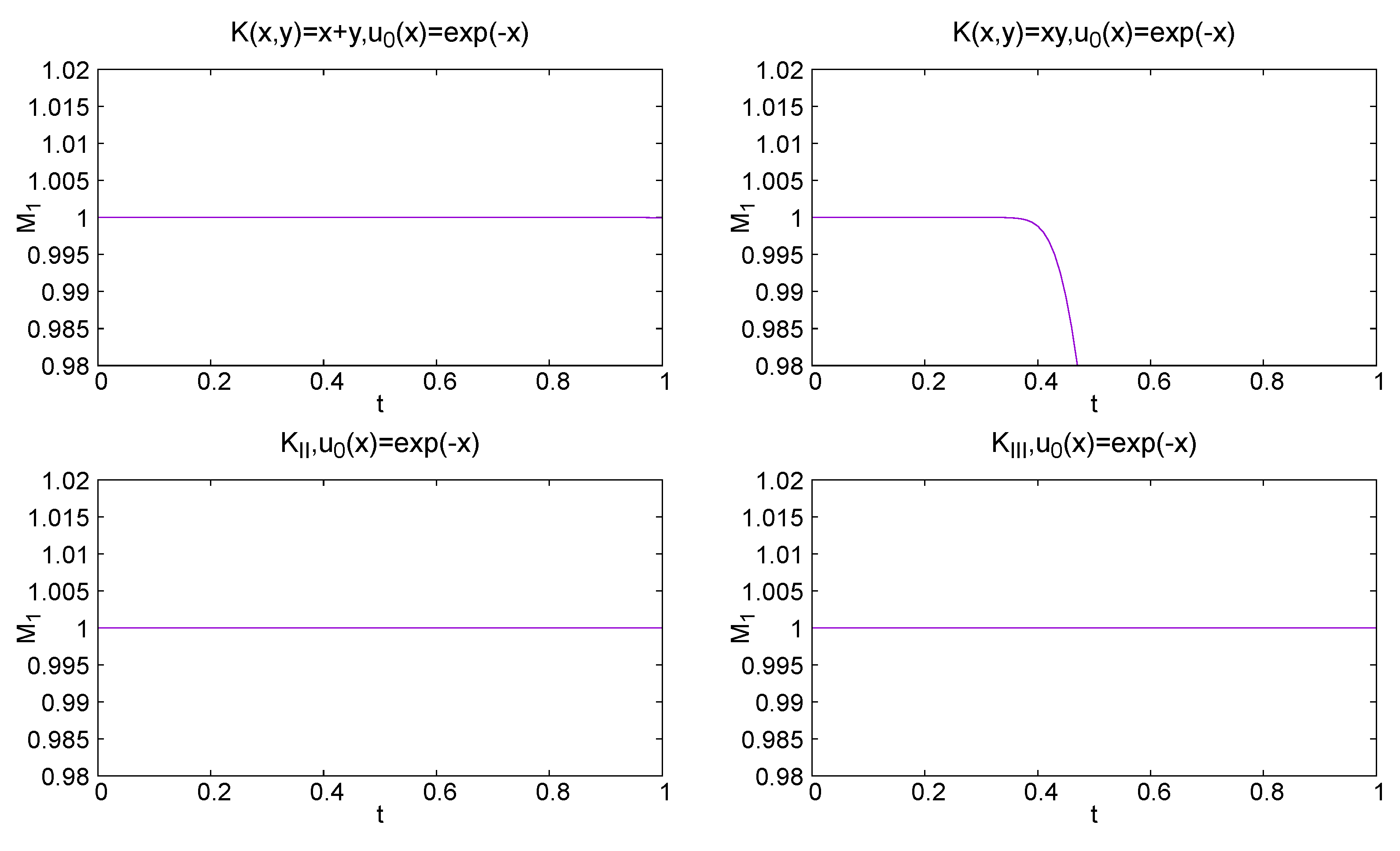
4. Mass Conservation Theorem

In this section, we state our main theorem, which gives a sufficient condition on the coagulation kernel K ( x , y ) and the weight function b ( x ) for the mass conservation property. We suppose that K ( x , y ) satisfies the properties (a1)–(a3) and
b C ( R + ) and b ( x ) 0 .
Furthermore, we assume that there exist some constants C 1 , C 2 > 0 , and the following conditions hold for all x , y R + :
(c1)
( x + y ) K ( x , y ) C 1 b ( x ) + x + 1 b ( y ) + y + 1 ,
(c2)
b ( x + y ) b ( x ) b ( y ) K ( x , y ) C 2 b ( y ) + y + 1 ( x + 1 ) + b ( x ) + x + 1 ( y + 1 ) .
For example, if the coagulation kernel is sublinear, i.e., there exists C > 0 such that K ( x , y ) C ( x + y + 1 ) for x , y R + , then conditions (c1) and (c2) hold for b ( x ) = x 2 .
When a weight function b ( x ) is given as in (12), the following proposition provides an example of a coagulation kernel that satisfies conditions (c1) and (c2).
Proposition 3.
Under the condition in (12), we suppose that c 0 and
b ( x + y ) b ( x ) b ( y ) + c 0 f o r a l l x , y R + ,
and suppose that the kernel
K ( x , y ) = b ( x ) + b ( y ) b ( x + y ) b ( x ) b ( y ) + x + y + c
is continuous on R + × R + . Then, it satisfies assumptions (a1)–(a3) and (c1) and (c2). In particular, if b as given in (12) is convex and c > b ( 0 ) , then (a1)–(a3) and (c1) and (c2) are satisfied.
Proof. 
From (13), conditions (c1) and (c2) are derived as follows:
( x + y ) K ( x , y ) = ( x + y ) b ( x ) + b ( y ) b ( x + y ) b ( x ) b ( y ) + x + y + c ( x + y ) b ( x ) + b ( y ) x + y = b ( x ) + b ( y ) ( b ( x ) + x + 1 ) ( b ( y ) + y + 1 ) ,
b ( x + y ) b ( x ) b ( y ) K ( x , y ) = b ( x + y ) b ( x ) b ( y ) b ( x ) + b ( y ) b ( x + y ) b ( x ) b ( y ) + x + y + c b ( x + y ) b ( x ) b ( y ) + x + y + c b ( x ) + b ( y ) b ( x + y ) b ( x ) b ( y ) + x + y + c = b ( x ) + b ( y ) b ( y ) + y + 1 ( x + 1 ) + b ( x ) + x + 1 ( y + 1 ) .
If b is convex and c > b ( 0 ) , then
b ( x + y ) b ( x ) b ( y ) + c > 0 f o r a l l x , y R + ,
holds from Proposition 5 in Appendix D and K C 0 ( R + × R + ) . □
Lemma 2.
We suppose that u is a classical solution of the SCE on [ 0 , T ] , and that (12) and (c2) hold. If M 1 ( 0 ) < and M b ( 0 ) < , there exists B > 0 such that M b ( t ) B for t [ 0 , T ] .
Proof. 
From Corollary 1 and (c2), taking into account Proposition 2, we have
t m b ( r , t ) 1 2 0 r 0 r b ( x + y ) b ( x ) b ( y ) K ( x , y ) u ( x , t ) u ( y , t ) d x d y C 2 2 0 r 0 r ( b ( y ) + y + 1 ) ( x + 1 ) + ( b ( x ) + x + 1 ) ( y + 1 ) u ( x , t ) u ( y , t ) d x d y = C 2 0 r 0 r b ( y ) + y + 1 ( x + 1 ) u ( x , t ) u ( y , t ) d x d y = C 2 0 r ( x + 1 ) u ( x , t ) d x 0 r b ( y ) + y + 1 u ( y , t ) d y = C 2 m 1 ( r , t ) + m 0 ( r , t ) m b ( r , t ) + m 1 ( r , t ) + m 0 ( r , t ) C 2 M 1 ( 0 ) + M 0 ( 0 ) m b ( r , t ) + M 1 ( 0 ) + M 0 ( 0 ) = C 2 A m b ( r , t ) + C 2 A 2 ,
where we set A : = M 1 ( 0 ) + M 0 ( 0 ) . By solving the differential inequality, we obtain
m b ( r , t ) m b ( r , 0 ) e C 2 A t + A ( e C 2 A t 1 ) M b ( 0 ) e C 2 A t + A ( e C 2 A t 1 ) B ,
where B : = ( A + M b ( 0 ) ) e C 2 A T . By taking r , we conclude that M b ( t ) B . □
Lemma 3.
We suppose that u is a classical solution of the SCE on [ 0 , T ] , and that (12) and (c1) and (c2) hold. If M 1 ( 0 ) < and M b ( 0 ) < , it holds that
lim r 0 t J [ u ] ( r , s ) d s = 0 for t [ 0 , T ] .
Proof. 
For r > 0 , we define
E 0 ( r ) : = ( x , y ) R 2 ; 0 x r , r x y , E 1 ( r ) : = ( x , y ) R 2 ; x 0 , y r 2 , E 1 ( r ) : = ( x , y ) R 2 ; y 0 , x r 2 .
Since E 0 ( r ) ( E 1 ( r ) E 1 ( r ) ) , we have
J [ u ] ( r , t ) = E 0 ( r ) x K ( x , y ) u ( x , t ) u ( y , t ) d x d y E 1 ( r ) ( x + y ) K ( x , y ) u ( x , t ) u ( y , t ) d x d y + E 1 ( r ) ( x + y ) K ( x , y ) u ( x , t ) u ( y , t ) d x d y = 2 E 1 ( r ) ( x + y ) K ( x , y ) u ( x , t ) u ( y , t ) d x d y 2 C 1 E 1 ( r ) b ( x ) + x + 1 b ( y ) + y + 1 u ( x , t ) u ( y , t ) d x d y = 2 C 1 0 b ( x ) + x + 1 u ( x , t ) d x r / 2 b ( y ) + y + 1 u ( y , t ) d y = 2 C 1 M b ( t ) + M 1 ( t ) + M 0 ( t ) r / 2 b ( y ) + y + 1 u ( y , t ) d y 2 C 1 B + M 1 ( 0 ) + M 0 ( 0 ) r / 2 b ( y ) + y + 1 u ( y , t ) d y ,
where the last inequality holds from Proposition 2 and Lemma 2.
Since
r / 2 b ( y ) + y + 1 u ( y , t ) d y = M b ( t ) m b r 2 , t + M 1 ( t ) m 1 r 2 , t + M 0 ( t ) m 0 r 2 , t ,
and the three terms on the right-hand side tend to zero as r , we obtain
lim r J [ u ] ( r , t ) = 0 for t [ 0 , T ] .
From (14), we also have
J [ u ] ( r , t ) 2 C 1 B + M 1 ( 0 ) + M 0 ( 0 ) 2 for r R + a n d t [ 0 , T ] .
By Lebesgue’s dominated convergence theorem [32], we obtain
lim r 0 t J [ u ] ( r , s ) d s = 0 t lim r J [ u ] ( r , s ) d s = 0 .
This completes the proof of Lemma 3. □
Lemma 3 guarantees that no mass flux can escape to infinity. Hence, we can prove the following mass conservation theorem using Lemma 3.
Theorem 2 (Mass conservation).
We suppose that u is a classical solution of the SCE on [ 0 , T ] , and that (12) and (c1) and (c2) hold. If M 1 ( 0 ) < and M b ( 0 ) < , then it holds that M 1 ( t ) = M 1 ( 0 ) and M b ( t ) B for t [ 0 , T ] , where B is a constant defined in Lemma 2.
Proof. 
The assertion M b ( t ) B has already been shown in Lemma 2. The other assertion M 1 ( t ) = M 1 ( 0 ) is shown as follows. For r > 0 and t [ 0 , T ] , integrating (7) with respect to x over [ 0 , r ] , we obtain
t m 1 ( r , t ) = 0 r x t u ( x , t ) d x = 0 r x J [ u ] ( x , t ) d x = J [ u ] ( r , t ) .
So, we have
m 1 ( r , t ) = m 1 ( r , 0 ) 0 t J [ u ] ( r , s ) d s .
Taking r and applying Lemma 3, we obtain
M 1 ( t ) = M 1 ( 0 ) f o r t [ 0 , T ] .
Hence, the proof is complete. □
As an application of this theorem, we can prove the following corollary, which is a special case of the results presented in [28,29].
Corollary 2.
We suppose that K satisfies (a1)–(a3) and there exists C > 0 such that
K ( x , y ) C ( x + y + 1 ) f o r x , y R + .
If u is a classical solution for the SCE on [ 0 , T ] and M 2 ( 0 ) < , then M 1 ( t ) = M 1 ( 0 ) and M 2 ( t ) < for t [ 0 , T ] .
Proof. 
It is clear that (c1) and (c2) hold with b ( x ) = x 2 because b ( x + y ) b ( x ) b ( y ) = 2 x y . Then, the assertion follows from Theorem 2. □

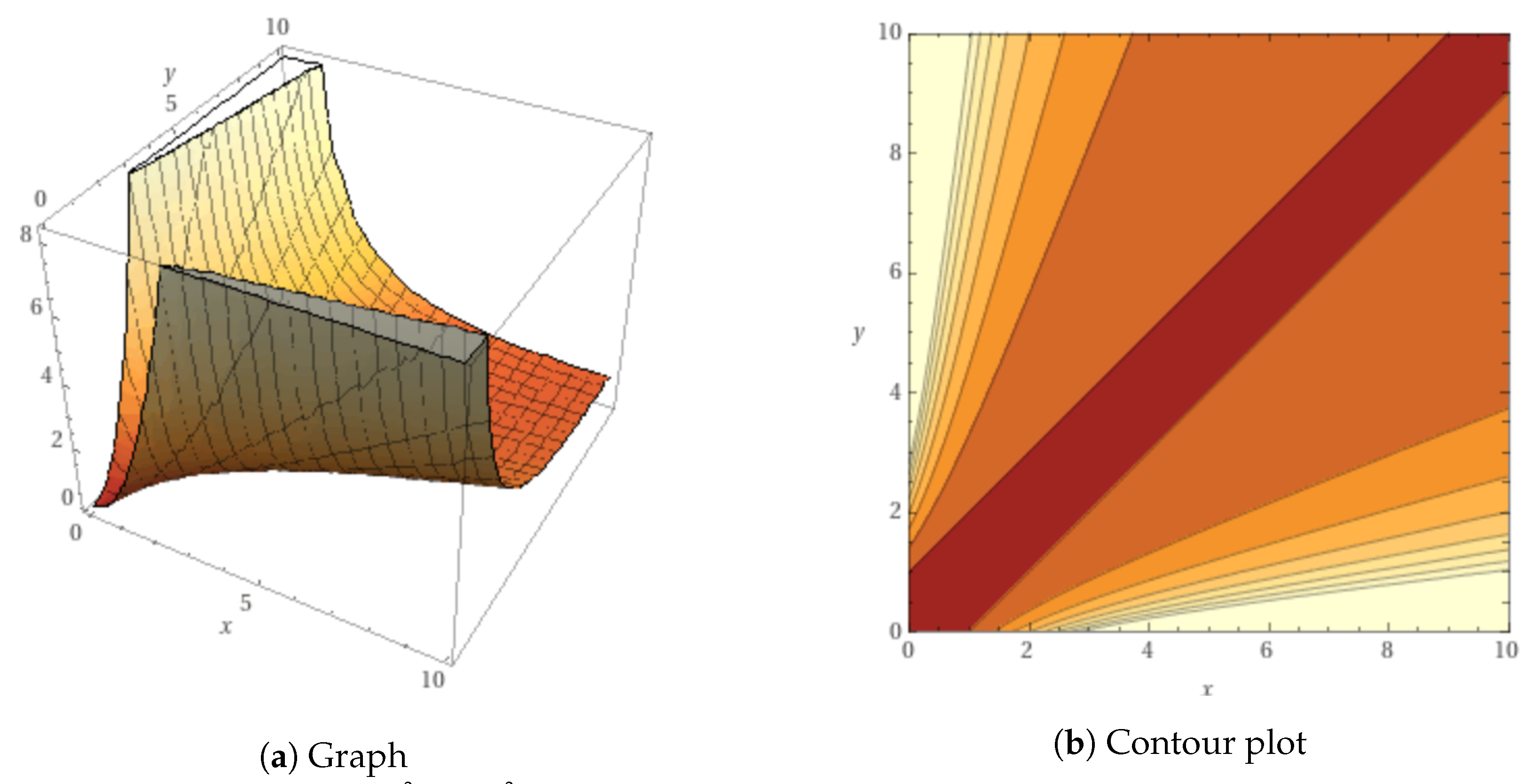
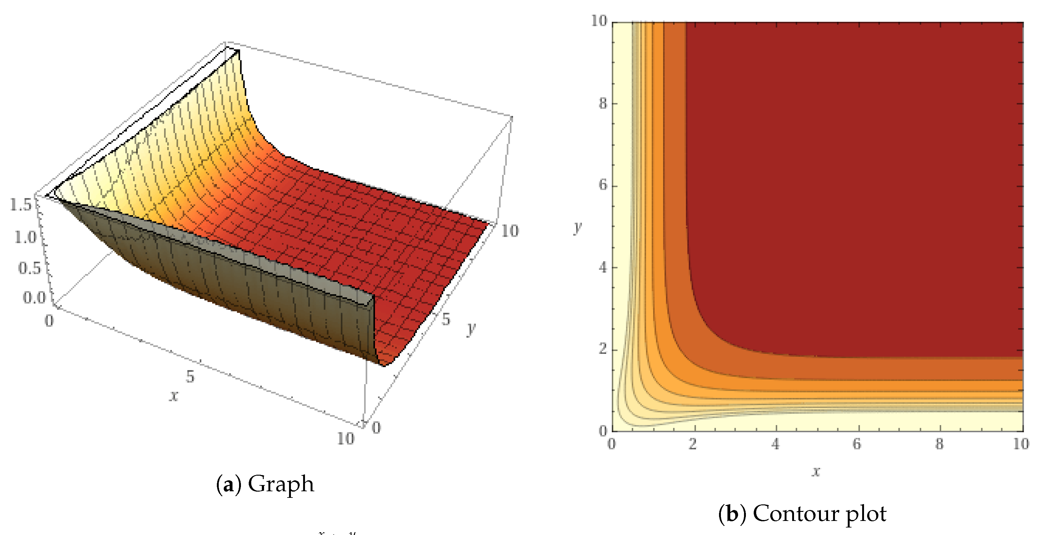
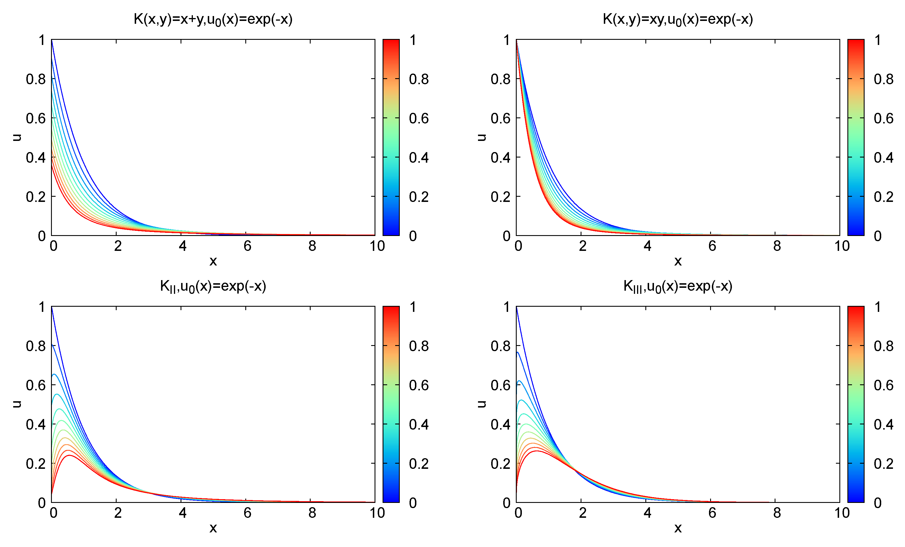
5. Examples of Mass-Conserving Kernels

As an application of Theorem 2 and Proposition 3, we provide several examples of kernels for which the mass conservation property holds but is not sublinear.

5.1. Polynomial Growth Kernel I

Setting b ( x ) = x p ( p N , p 3 ) and c 0 , we apply Proposition 3. Then, we have
K I ( x , y ) = x p + y p ( x + y ) p x p y p + x + y + c = x p + y p n = 1 p 1 p n x p n y n + x + y + c ,
where p n is a binomial coefficient. We note that this kernel is continuous on R + × R + , even when c = 0 (see (17)). Since it satisfies (c1) and (c2), if M p ( 0 ) < , then the mass is conserved. However, for y = x ( p 2 ) , it satisfies
K I x , x ( p 2 ) = x p + x p ( p 2 ) ( p + 1 ) x + O ( 1 ) = 1 p + 1 x p 1 + O ( x p 2 ) as x .
This means that the kernel K I ( x , y ) has a polynomial growth of the order of x p 1 along the curve y = x ( p 2 ) . This is an example of a mass-conserving kernel that does not have sublinear growth.

5.2. Polynomial Growth Kernel II

As in the previous example, we can construct another more simple mass-conserving kernel with polynomial growth. Again, we set b ( x ) = x p ( p N , p 3 ) and define
K I I ( x , y ) = x p + y p x y ( x + y ) p 2 + x + y .
We note that K C 0 ( R + × R + ) holds since x p + y p x + y is continuous in R + × R + . Furthermore, using the inequality
3 p 2 n 1 p n p p 2 n 1 for 1 n p 1 ,
we have
3 x y ( x + y ) p 2 ( x + y ) p x p y p p x y ( x + y ) p 2 .
Then, we obtain
K I I ( x , y ) x p + y p 1 p { ( x + y ) p x p y p } + x + y 1 p K I ( x , y ) | c = 0 .
Since K I ( x , y ) satisfies conditions (c1) and (c2), K I I ( x , y ) follows the same conditions.
For y = x ( p 2 ) , it satisfies
K I I ( x , x ( p 2 ) ) = x p + x p ( p 2 ) 2 x + O ( 1 ) = 1 2 x p 1 + O ( x p 2 ) a s x .
In particular, when p = 3 , it becomes
K I I ( x , y ) | p = 3 = x 2 x y + y 2 x y + 1 ,
which exhibits a quadratic growth along the curve y = x 1 :
K I I ( x , x 1 ) | p = 3 = 1 2 x 2 + O ( x ) as x .
We show a graph and a contour plot of K I I ( x , y ) | p = 3 in Figure 1.

5.3. Exponential Growth Kernel

We set b ( x ) = e x and c = 2 and apply Proposition 3. Then, we have
K I I I ( x , y ) = e x + e y e x + y e x e y + x + y + 2 = e x + e y ( e x 1 ) ( e y 1 ) + x + y + 1 ,
where we chose c = 2 because K I I I is continuous at ( x , y ) = ( 0 , 0 ) only if c > 1 . Since K I I I C 0 ( R + × R + ) , if M b ( 0 ) < it means that
0 e x u ( x , 0 ) d x < ,
so the mass is conserved.
Along the curve y = log ( 1 + e α x ) ( α 1 ) , it satisfies
K I I I ( x , log ( 1 + e α x ) ) = e x + 1 + e α x ( e x + 1 ) ( 1 + e α x 1 ) + x + log ( 1 + e α x ) + 1 = e x + 1 + e α x e ( 1 α ) x ( 1 + e x ) + x + log ( 1 + e α x ) + 1 = e x + O ( 1 ) x + O ( 1 ) = e x x + O 1 x a s x .
This is an example of an exponentially growing and mass-conserving kernel. We provide a graph and a contour plot of K I I I ( x , y ) in Figure 2.

5.4. Discussion

In the introduction, we discussed the conservation of mass and gel phenomena for various types of kernels. Here, using the numerical simulation, we compare our new kernels that satisfy (c1) and (c2) with some previously known kernels. For the numerical simulation, we employ the finite volume method proposed by Filbet and Laurençot [21].
In Figure 3, we can see the time evolution of the solution profile u ( x , t ) with an initial condition u 0 ( x ) = e x for previously known kernels K ( x , y ) = x + y and K ( x , y ) = x y , as well as our chosen kernels K I I ( x , y ) | p = 3 and K I I I ( x , y ) . In these numerical computations, we truncate x R + to the interval [ 0 , R ] with R = 200.0 and divide [ 0 , R ] as 0 = x 0 < x 1 < . . . < x n = R , where x i = R ( i / n ) 2 and n = 500 . However, we only show the interval x [ 0 , 10 ] in the figures. For time, we compute t [ 0 , T ] with T = 1.0 and Δ t = 0.01 . The color bars on the right side of the figures represent the corresponding time t.
In Figure 4, the time evolution of the total mass M 1 ( t ) is plotted. As expected, mass conservation holds for the kernel K ( x , y ) = x + y (Corollary 2), whereas it is not conserved for K ( x , y ) = x y (Proposition 4). We also observe that mass is conserved for our chosen kernels: K I I ( x , y ) | p = 3 and K I I I ( x , y ) . For the mass-conserving kernel, the plot shows a straight line throughout the time interval, whereas for the non-conserving kernel, the straight line breaks, indicating the occurrence of the gel phenomenon.

6. Conclusions

In this paper, we proposed the generalized moment method based on the truncated moment identity (Theorem 1). Using this generalized moment, in Section 4, we studied a sufficient condition of the mass conservation property for the coagulation kernel K ( x , y ) and the initial condition (Theorem 2). As a result of our main theorem, we provided several examples of new kernels, along with some numerical illustrations, where mass conservation was achieved.
In most previous works, the focus has been on studying mass conservation and gelation phenomena for homogeneous kernels, i.e., K ( λ x , λ y ) = λ α K ( x , y ) , or under the assumption that K ( x , y ) admits an inequality with a homogeneous kernel. Roughly speaking, if α 1 , mass is conserved, and if α > 1 , gelation occurs [15,26,28,29].
On the other hand, the mass-conserving kernels discussed in Section 5 are not homogeneous and cannot be bounded from above by a linear-order growth function, i.e., (15) does not hold for any C > 0 . Furthermore, we also demonstrated that the kernels K I ( x , y ) and K I I ( x , y ) exhibit polynomial growth, whereas K I I I ( x , y ) exhibits exponential growth along specific curves such as x .
In addition, our main result, Theorem 2, strongly suggests that the occurrence of mass conservation or gelation depends not only on the growth properties of the coagulation kernel but also on the boundedness of the initial generalized moment M b ( 0 ) . In this sense, it would be interesting to further investigate gelation phenomena using the generalized moment method.

Author Contributions

M.S.I. and M.K. contributed to the conceptualization, analysis, and writing—original draft preparation. H.M. contributed to the analysis and simulations. All authors have read and agreed to the published version of the manuscript.

Funding

M.S.I. was the recipient of the MEXT LocSEES scholarship.

Data Availability Statement

The data for the numerical simulations in this study are available from the authors.

Conflicts of Interest

The authors declare no conflict of interest.

Appendix A. Derivation of Flux

A mass flux density (often simply called a mass flux) J ( x 0 , t ) R for x 0 > 0 is defined as the rate of mass flow in the size domain R + across x = x 0 from the side [ 0 , x 0 ) to the other side ( x 0 , ) , which must satisfy
d d t 0 x 0 y u ( y , t ) d y = J ( 0 , t ) J ( x 0 , t ) = J ( x 0 , t ) ,
d d t x 0 y u ( y , t ) d y = J ( x 0 , t ) lim r J ( r , t ) ,
where we set J ( 0 , t ) = 0 since we consider only coagulation. Specifically, from (A1), we obtain the conservation law (2). Furthermore, from (A2), the mass conservation M 1 ( t ) = M 1 ( 0 ) is expected if lim r J ( r , t ) = 0 . This is the key idea of the proof of Theorem 2.
In this section, we derive the mass flux from the viewpoint of the elementary physical process. For the mass distribution u ( x , t ) 0 , the mass distribution is represented by x u ( x , t ) . We fix x 0 > 0 and take any particle of mass y ( 0 , x 0 ) and another particle of mass z ( x 0 , ) . For the particle of mass y, we consider a coagulation rate R ( y , z , t ) 0 of the mass change y z per unit time by coagulating with a particle of mass z y , which is given by
R ( y , z , t ) = K ( y , z y ) u ( z y , t ) for 0 < y < x 0 < z .
The mass flux J ( x 0 , t ) is given by
J ( x 0 , t ) = 0 x 0 y u ( y , t ) x 0 R ( y , z , t ) d z d y = 0 x 0 x 0 y u ( y , t ) K ( y , z y ) u ( z y , t ) d z d y = 0 x 0 x 0 y y K ( y , z ) u ( y , t ) u ( z , t ) d z d y .
This gives Formula (3), and SCE (1) is derived from (2) and Proposition 1.

Appendix B. A Simple Proof of Gelation Phenomena

In this appendix, we provide proof of the occurrence of gelation for the coagulation kernel K ( x , y ) a x y . This type of proof is provided in [26,27]. We include it here for the reader’s convenience.
Proposition 4.
We suppose that K ( x , y ) a x y , with a > 0 , and u is a weak solution of SCE on [ 0 , T ] , with M 1 ( 0 ) < . Then, we obtain
M 1 ( t ) 2 M 0 ( 0 ) a t for t ( 0 , T ] .
In particular, it implies that a gelation M 1 ( t ) < M 1 ( 0 ) should occur if t * < t T , where
t * : = 2 M 0 ( 0 ) a M 1 ( 0 ) 2 .
Proof. 
From the truncated moment identity (Theorem 1) with b ( x ) = 1 , we have
t m 0 ( r , t ) a 2 0 r 0 r x x y u ( x , t ) u ( y , t ) d y d x a 0 r r x x y u ( x , t ) u ( y , t ) d y d x a 2 0 r 0 x y u ( x , t ) u ( y , t ) d y d x = a 2 m 1 ( r , t ) M 1 ( t ) .
Integrating within ( 0 , t ) , we obtain
m 0 ( r , t ) m 0 ( r , 0 ) a 2 0 t m 1 ( r , s ) M 1 ( s ) d s for r R + , t [ 0 , T ] .
From Proposition 2 and Fatou’s lemma, taking r , we have
M 0 ( t ) M 0 ( 0 ) a 2 lim r 0 t m 1 ( r , s ) M 1 ( s ) d s a 2 0 t lim r m 1 ( r , s ) M 1 ( s ) d s = a 2 0 t M 1 ( s ) 2 d s for t [ 0 , T ] .
This implies that,
M 0 ( 0 ) M 0 ( 0 ) M 0 ( t ) a 2 0 t M 1 ( s ) 2 d s a 2 0 t M 1 ( t ) 2 d s = a t 2 M 1 ( t ) 2 ,
where we have used that M 1 ( t ) is non-increasing (Proposition 2). Hence, we have proven the assertion. □

Appendix C. Supplementary Lemma

Lemma 4.
Let I = [ a , b ] for a < b , and let D : = { ( x , y ) R 2 ; a y x b } . We suppose that f ( x , y ) satisfies f C 0 ( D ) and f x C 0 ( D ) , and define g ( x ) : = a x f ( x , y ) d y for x I . Then, g C 1 ( I ) , and it holds that
g ( x ) = f ( x , x ) + a x f x ( x , y ) d y f o r x I .
Proof. 
For x I , since f ( x , y ) = f ( y , y ) + y x f x ( z , y ) d z , we have
g ( x ) = a x f ( y , y ) + y x f x ( z , y ) d z d y = a x f ( z , z ) d z + a x a z f x ( z , y ) d y d z = a x f ( z , z ) + a z f x ( z , y ) d y d z .
This implies that g C 1 ( I ) and (A3). □

Appendix D. Convexity and Superadditivity

In this appendix, we provide some brief information about the convexity and superadditivity of a function defined on R + .
Definition 3.
Let b ( x ) be a function, b : R + R . Then,
  • b is called convex on R + if
    b ( 1 θ ) x + θ y ( 1 θ ) b ( x ) + θ b ( y ) for x , y R + and θ [ 0 , 1 ] .
  • b is called superadditive on R + if
    b ( x + y ) b ( x ) + b ( y ) for x , y R + .
Proposition 5.
If b is convex on R + , the following inequality holds
b ( x + y ) b ( x ) + b ( y ) b ( 0 ) for x , y R + .
In particular, if b is convex on R + and b ( 0 ) 0 , then b is superadditive on R + .
Proof. 
When x = 0 or y = 0 , (A4) holds. If x > 0 and y > 0 , we have
b ( x ) = b y x + y 0 + x x + y ( x + y ) y x + y b ( 0 ) + x x + y b ( x + y ) .
Similarly, we have
b ( y ) x x + y b ( 0 ) + y x + y b ( x + y ) .
Adding these inequalities, we obtain (A4). □

References

  1. Pesmazoglou, I.; Kempf, A.; Navarro-Martinez, S. Stochastic modelling of particle aggregation. Int. J. Multiph. Flow 2016, 80, 118–130. [Google Scholar] [CrossRef]
  2. Ernst, M.; Ziff, R.M.; Hendriks, E. Coagulation processes with a phase transition. J. Colloid Interface Sci. 1984, 97, 266–277. [Google Scholar] [CrossRef]
  3. Ziff, R.M. Kinetics of polymerization. J. Stat. Phys. 1980, 23, 241–263. [Google Scholar] [CrossRef]
  4. Drake, R.L. A general mathematical survey of the coagulation equation. Int. Rev. Aerosol Phys. Chem. 1972, 3, 201–376. [Google Scholar]
  5. Seinfeld, J.H. ES and T books: Atmospheric chemistry and physics of air pollution. Environ. Sci. Technol. 1986, 20, 863. [Google Scholar] [CrossRef] [PubMed]
  6. Kumar, J.; Warnecke, G.; Peglow, M.; Heinrich, S. Comparison of numerical methods for solving population balance equations incorporating aggregation and breakage. Powder Technol. 2009, 189, 218–229. [Google Scholar] [CrossRef]
  7. Zidar, M.; Kuzman, D.; Ravnik, M. Characterisation of protein aggregation with the Smoluchowski coagulation approach for use in biopharmaceuticals. Soft Matter 2018, 14, 6001–6012. [Google Scholar] [CrossRef]
  8. Tavaré, S. Line-of-descent and genealogical processes, and their applications in population genetics models. Theor. Popul. Biol. 1984, 26, 119–164. [Google Scholar] [CrossRef]
  9. Family, F.; Landau, D.P. Kinetics of Aggregation and Gelation; Elsevier: Amsterdam, The Netherlands, 2012. [Google Scholar]
  10. Silk, J.; White, S.D. The development of structure in the expanding universe. Astrophys. J. 1978, 223, L59–L62. [Google Scholar] [CrossRef]
  11. Banakar, Z.; Tavana, M.; Huff, B.; Di Caprio, D. A bank merger predictive model using the Smoluchowski stochastic coagulation equation and reverse engineering. Int. J. Bank Mark. 2018, 36, 634–662. [Google Scholar] [CrossRef]
  12. Smoluchowski, M. Drei vorträge über diffusion, brownsche molekularbewegung und koagulation von kolloidteilchen. Pisma Marian. Smoluchowskiego 1927, 2, 530–594. [Google Scholar]
  13. Müller, H. Zur allgemeinen Theorie ser raschen Koagulation. Kolloidchem. Beih. 1928, 27, 223–250. [Google Scholar] [CrossRef]
  14. Smit, D.; Hounslow, M.; Paterson, W. Aggregation and gelation—I. Analytical solutions for CST and batch operation. Chem. Eng. Sci. 1994, 49, 1025–1035. [Google Scholar] [CrossRef]
  15. Aldous, D.J. Deterministic and stochastic models for coalescence (aggregation and coagulation): A review of the mean-field theory for probabilists. Bernoulli 1999, 5, 3–48. [Google Scholar] [CrossRef]
  16. Estrada, P.R.; Cuzzi, J.N. Solving the coagulation equation by the moments method. Astrophys. J. 2008, 682, 515–526. [Google Scholar] [CrossRef]
  17. Menon, G.; Pego, R.L. Approach to self-similarity in Smoluchowski’s coagulation equations. Commun. Pure Appl. Math. A J. Issued Courant Inst. Math. Sci. 2004, 57, 1197–1232. [Google Scholar] [CrossRef]
  18. Van Dongen, P.; Ernst, M. Scaling solutions of Smoluchowski’s coagulation equation. J. Stat. Phys. 1988, 50, 295–329. [Google Scholar] [CrossRef]
  19. Kruis, F.E.; Maisels, A.; Fissan, H. Direct simulation Monte Carlo method for particle coagulation and aggregation. Am. Inst. Chem. Eng. J. 2000, 46, 1735–1742. [Google Scholar] [CrossRef]
  20. Mahoney, A.W.; Ramkrishna, D. Efficient solution of population balance equations with discontinuities by finite elements. Chem. Eng. Sci. 2002, 57, 1107–1119. [Google Scholar] [CrossRef]
  21. Filbet, F.; Laurençot, P. Numerical simulation of the Smoluchowski coagulation equation. SIAM J. Sci. Comput. 2004, 25, 2004–2028. [Google Scholar] [CrossRef]
  22. Sadri, K.; Ebrahimi, H. New Method for Homogeneous Smoluchowski Coagulation Equation. J. Appl. Comput. Math. 2015, 4, 2. [Google Scholar]
  23. Makino, J.; Fukushige, T.; Funato, Y.; Kokubo, E. On the mass distribution of planetesimals in the early runaway stage. New Astron. 1998, 3, 411–417. [Google Scholar] [CrossRef]
  24. Tanaka, H.; Inaba, S.; Nakazawa, K. Steady-state size distribution for the self-similar collision cascade. Icarus 1996, 123, 450–455. [Google Scholar] [CrossRef]
  25. McLeod, J. On an infinite set of non-linear differential equations. Q. J. Math. 1962, 13, 119–128. [Google Scholar] [CrossRef]
  26. Escobedo, M.; Mischler, S.; Perthame, B. Gelation in coagulation and fragmentation models. Commun. Math. Phys. 2002, 231, 157–188. [Google Scholar] [CrossRef]
  27. Laurençot, P. On a class of continuous coagulation-fragmentation equations. J. Differ. Equ. 2000, 167, 245–274. [Google Scholar] [CrossRef]
  28. Escobedo, M.; Mischler, S.; Ricard, M.R. On self-similarity and stationary problem for fragmentation and coagulation models. Ann. l’Inst. Henri Poincaré C Anal. Non Linéaire 2005, 22, 99–125. [Google Scholar] [CrossRef]
  29. Escobedo, M.; Mischler, S. Dust and self-similarity for the Smoluchowski coagulation equation. Ann. l’Inst. Henri Poincaré C Anal. Non Linéaire 2006, 23, 331–362. [Google Scholar] [CrossRef]
  30. Norris, J.R. Smoluchowski’s coagulation equation: Uniqueness, nonuniqueness and a hydrodynamic limit for the stochastic coalescent. Ann. Appl. Probab. 1999, 9, 78–109. [Google Scholar] [CrossRef]
  31. Pego, R.L. Dynamics and scaling in models of coarsening and coagulation. In Proceedings of the Pan-American Advanced Studies Institute (VIII America’s Conference on Differential Equations), Mexico City, Mexico, 15–17 October 2009. [Google Scholar]
  32. Evans, L.C.; Gariepy, R.F. Measure Theory and Fine Properties of Functions; CRC Press: Boca Raton, FL, USA, 2015. [Google Scholar]
Figure 1. K I I ( x , y ) | p = 3 = x 2 x y + y 2 x y + 1 .
Mathematics 11 02770 g001
Figure 2. K I I I ( x , y ) = e x + e y ( e x 1 ) ( e y 1 ) + x + y + 1 .
Mathematics 11 02770 g002
Figure 3. Solution graphs for different kernels. The color bar on the right represents the time t.
Mathematics 11 02770 g003
Figure 4. Graph of M 1 for different kernels.
Mathematics 11 02770 g004
Disclaimer/Publisher’s Note: The statements, opinions and data contained in all publications are solely those of the individual author(s) and contributor(s) and not of MDPI and/or the editor(s). MDPI and/or the editor(s) disclaim responsibility for any injury to people or property resulting from any ideas, methods, instructions or products referred to in the content.

