A Novel Data-Driven Feature Extraction Strategy and Its Application in Looseness Detection of Rotor-Bearing System

Abstract

During the service of rotating machinery, the pedestal bolts are prone to looseness due to the vibration environment, which affects the performance of rotating machinery and generate potential safety hazard. To monitor the occurrence and deterioration of the pedestal looseness in time, this paper proposes a data-driven diagnosis strategy for the rotor-bearing system. Firstly, the finite element model of a rotor-bearing system is established, which considers the piecewise nonlinear force caused by pedestal looseness. Taking the vibration response as output and periodic unbalanced force as input, the system’s NARX (Nonlinear Auto-Regressive with exogenous inputs) model is identified. Then GALEs (Generalized Associated Linear Equations) are used to evaluate NOFRFs (Nonlinear Output Frequency Response Functions) of the NARX model. Based on the first three-order NOFRFs, the analytical expression of the second-order optimal weighted contribution rate is derived and used as a new health indicator. The simulation results show that compared with the conventional NOFRFs-based health indicator, the new indicator is more sensitive to weak looseness. Finally, a rotor-bearing test rig was built, and the pedestal looseness was performed. The experiment results show that as the degree of looseness increases, the new indicator SRm shows a monotonous upward trend, increasing from 0.48 in no looseness to 0.90 in severe looseness, a rise of 89.7%. However, the traditional indicator Fe2 has no monotonicity, which further verifies the sensitivity of the first three-order NOFRFs-based second-order optimal weighted contribution rate and the effectiveness of the proposed data-driven feature extraction strategy.

1. Introduction

Affected by installation, vibration environment, and structural deformation, looseness is prone to occur between the bearing seat and foundation (or casing) in rotating machinery [1]. When the looseness fault becomes serious, the vibration of rotating parts will exceed the allowable value, which is likely to cause other coupling faults, such as rub impact [2,3]. Therefore, early detection of looseness is essential to the service life and safe operation of rotating machinery.

The study on the fault feature extraction of looseness in rotor-bearing systems can be divided into three categories. The first is the feature extraction based on the physical model and failure mechanism. By exploring the vibration characteristics of the rotor-bearing system caused by looseness, the corresponding fault diagnosis methods are proposed. Jiang [4] proposed to linearize the nonlinear model of a rotor-bearing-pedestal system and use the difference between the linearized model and the nonlinear model as an indicator to measure the degree of nonlinearity caused by pedestal looseness. Zhang [5] considered nonlinear support and loss foundation when modelling a rotor-bearing system and analyzed the influence of the two kinds of faults on the transient and steady-state response when the two faults exist alone or coupled with each other. Ma [6] established a rotor-bearing finite element model considering pedestal looseness and separately considered the influence of the pedestal displacement and looseness gap on dynamics. Lu [7] established a 7-DOF dynamic model considering the pedestal looseness coupling of the ball bearing and used the modified proper orthogonal decomposition method to reduce the model. Yang [8] established a 3-DOF rotor model coupling unbalance, rub-impact, loose base, and rotor geometric nonlinearity and analyzed the influence of coupled faults and geometric nonlinearity on the resonance characteristics.

For complex rotor systems, sometimes it is impossible to establish an accurate physical model. The second method is based on signal processing to extract the looseness features from the vibration signal directly. A [9] proposed to combine ensemble empirical mode decomposition and Hilbert transform to extract looseness features from the vibration signal and orbit of the direct-drive wind turbine. The results show that the vibration response caused by the front and rear bearings under the same looseness gap is also very different. An [10] also used variational mode decomposition to extract the looseness features, and the results showed that the steady-state components of the vibration signal extracted have obvious amplitude modulation. Lee [11] used the Hilbert-Huang transform to extract the fault time-frequency characteristics of eccentric wear and pedestal looseness in the rotor system. The results show that when eccentric wear occurs, there is a noticeable impact signal. When the looseness occurs, there are non-periodic intermittent shock and friction signals. However, the signal processing-based fault features extraction methods are seriously affected by working conditions. Therefore, the sensitive features extracted from the signal do not necessarily reflect the changes in system nonlinearity.

Conventional detection methods based on physical models and signal processing are limited in real-time monitoring. The third method is based on data-driven dynamic modeling [12]. Data-driven models are mainly divided into two categories. The first is to directly use output response to identify dynamics models, such as AR (autoregressive) model [13] and ARMA (autoregressive moving average) model [14]. The second is to consider the external input, such as Volterra series models [15], Hammerstein models [16], NARMAX (nonlinear autoregressive moving average with exogenous inputs) model [17], and NARX (Nonlinear autoregressive with exogenous inputs) model [18]. When the terms of the data-driven model are determined in advance, the coefficients of the terms can be used as the features [19]. However, the number and form of model terms are uncertain in many cases, and the term coefficients cannot be used as fault features. Therefore, the weak fault feature extraction of the data-driven model is also an urgent problem to be solved.

For the problem, a novel data-driven fault feature extraction method is proposed. The first step is to establish the NARX model based on the simulation data or experimental data of a rotor-bearing system and then use the GALEs (Generalized Associated Linear Equations) to evaluate the NOFRFs (Nonlinear Output Frequency Response Functions) of the NARX model [20]. To extract more sensitive health indicators from NOFRFs, this paper proposes a weighted contribution rate based on the first three-order NOFRFs. The analytical expression of the second-order optimal weighted contribution rate of NOFRFs is derived in detail. The effectiveness of the novel health indicator is verified by simulation and experiment. Finally, the second-order optimal weighted contribution rate of NOFRFs is used to measure the pedestal looseness of the rotor-bearing system.

The organization of this paper is as follows. Section 2 is the theoretical basis, including how to obtain the NOFRFs from the NARX model using the GALEs and the theoretical derivation of the second-order optimal weighted contribution rate of NOFRFs. Section 3 is the dynamic simulation and analysis of a rotor-bearing system with pedestal looseness, including the establishment of a data-driven model and the measurement of looseness using the second-order optimal weighted contribution rate of NOFRFs. Section 4 is the experimental verification based on a rotor-bearing system test rig. Section 5 is the conclusions.

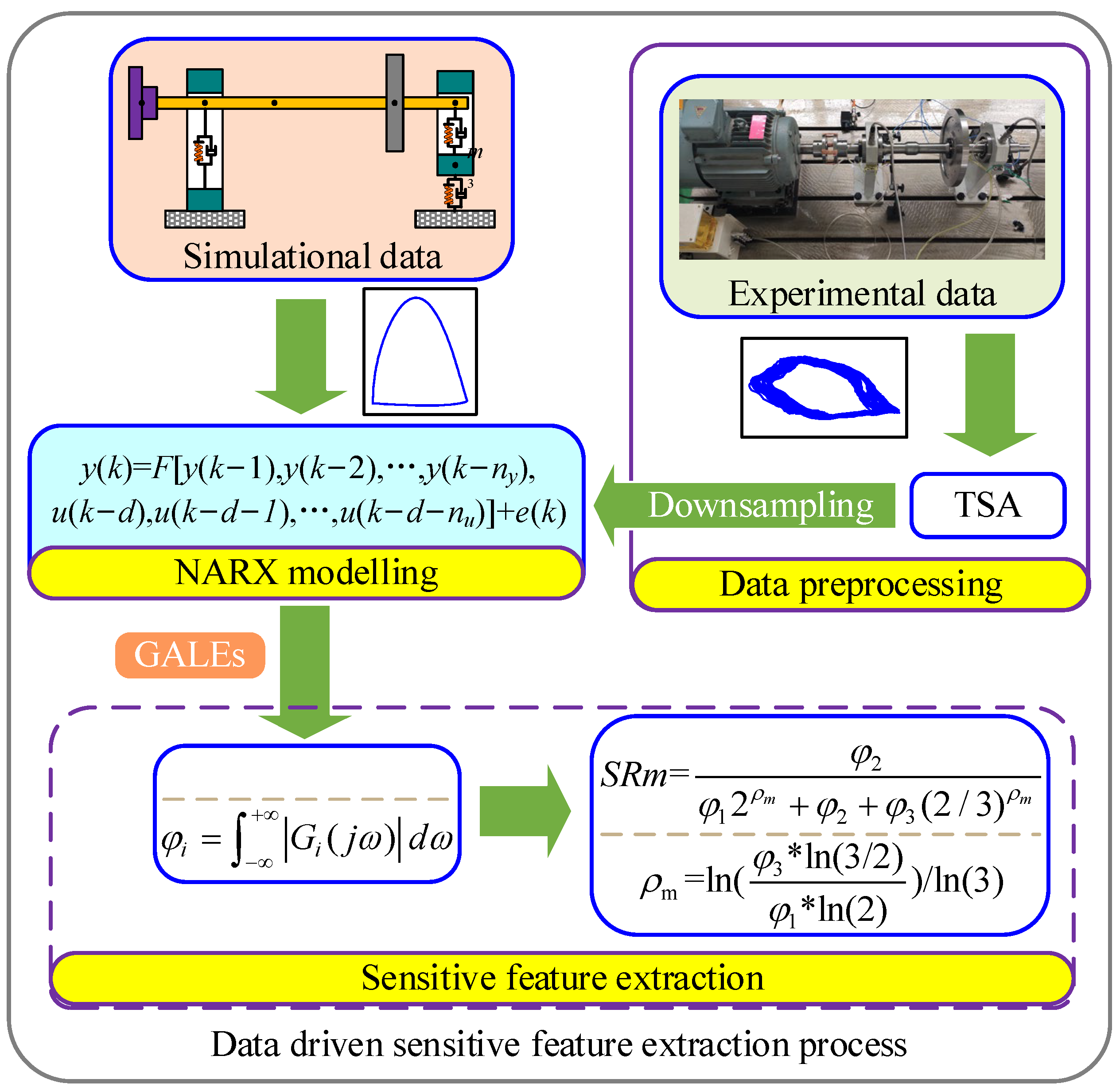
2. Data-Driven Feature Extraction

This paper mainly uses the NARX model to conduct the data-driven modeling of a rotor-bearing system. In engineering practice, the NARX model can represent a large class of nonlinear systems. The structure of a discrete single-input and single-output NARX model is [21]:

$$y\left(k\right)={\displaystyle \sum _{m=1}^M{\displaystyle \sum _{p=0}^m{\displaystyle \sum _{k_1,k_{p+q}=1}^K{c}_{p,q}\left(k_1,\cdots ,k_{p+q}\right)}}}{\displaystyle \prod _{i=1}^{p}y\left(k-k_i\right)}{\displaystyle \prod _{i=p+1}^{p+q}u\left(k-k_i\right)}$$

(1)

where M and K are integers, k represents discrete time, p + q = m and ${\displaystyle {\sum }_{k_1,k_{p+q}=1}^K=}$ ${\displaystyle {\sum }_{k_1=1}^K\cdots {\displaystyle {\sum }_{k_{p+q}=1}^K;}}$ $c_{p,q}\left(k_1,\cdots ,k_{p+q}\right)$ are the coefficients of the model terms. y(k) and u(k) represent the discrete output and input, respectively.

After the NARX model identification based on the real-time or historical vibration data, the Model Predicted Output (MPO) method is used to verify the model’s effectiveness. Then the GALEs method mentioned in Ref. [20] is used to decompose the NARX model and obtain the analytical expression of the system’s first N-order output y_n(k). Aiming at the general NARX model structure represented by Equation (1), the specific decomposition of GALEs is

$$\begin{array}{l}{y}_n\left(k\right)-{\displaystyle \sum _{k_1=1}^K{c}_{1,0}\left(k_1\right)y_n\left(k-k_1\right)}={\displaystyle \sum _{k_1,k_n=1}^K{c}_{0,n}\left(k_1,\cdots ,k_n\right)}\\ \times {\displaystyle \prod _{i=1}^{n}u\left(k-k_i\right)}+{\displaystyle \sum _{q=1}^{n-1}{\displaystyle \sum _{p=1}^{n-q}{\displaystyle \sum _{k_1,k_{p+q}=1}^K{c}_{p,q}\left(k_1,\cdots ,k_{p+q}\right)y_{n-q,p}^K\left(k\right)}}}\\ \times {\displaystyle \prod _{i=p+1}^{p+q}u\left(k-k_i\right)}+{\displaystyle \sum _{p=2}^n{\displaystyle \sum _{k_1,k_p=1}^K{c}_{p,0}\left(k_1,\cdots ,k_p\right)y_{n,p}^K\left(k\right)}}\end{array}$$

(2)

where n = 1, …, N, $K=\left(k_1,\dots ,k_{p+q}\right)$ represents the integer set of delay corresponding to coefficients $c_{p,q}\left(k_1,\cdots ,k_{p+q}\right)$.

$$\left\{\begin{array}{l}{y}_{n,p}^{\mathbf{K}}\left(k\right)={\displaystyle \sum _{i=1}^{n-(p-1)}{y}_i\left(k-k_p\right)y_{n-i,p-1}^{\mathbf{K}}\left(k\right)}\\ y_{n,1}^{\mathbf{K}}\left(k\right)=y_n\left(k-k_1\right)\end{array}\right.$$

(3)

The NARX model that satisfies the MPO criterion can be expanded to any order. At this time, the NOFRFs of the NARX model can be obtained from the GALEs as [22]

$$G_n\left(\mathrm{j}\omega \right)=\frac{Y_n\left(\mathrm{j}\omega \right)}{U_n\left(\mathrm{j}\omega \right)}$$

(4)

where the nth (n = 1, …, N) order output spectra Y_n(jω) and the input spectra U_n(jω) can be obtained from the Discrete Time Fourier Transform (DTFT) of y_n(k) and uⁿ(k), respectively. At this time, the output spectrum of the nonlinear system can be expressed as

$$Y\left(\mathrm{j}\omega \right)\approx {\displaystyle \sum _{n=1}^N{Y}_n\left(\mathrm{j}\omega \right)}={\displaystyle \sum _{n=1}^N{G}_n\left(\mathrm{j}\omega \right)U_n\left(\mathrm{j}\omega \right)}$$

(5)

Previously, identifying NOFRFs under harmonic excitation required two excitations with different excitation intensities but the same excitation frequency combining the least square method, which limits the application of NOFRFs in the fault diagnosis of rotating machinery. For the GALEs method, the NOFRFs can be obtained only by the NARX model obtained from one harmonic excitation, which significantly facilitates the application of NOFRFs in engineering. NOFRFs can directly characterize the nonlinearity of a system, but NOFRFs are multi-valued functions, and some orders of NOFRFs may be not sensitive and effective. Therefore, it is necessary to further extract sensitive features from the obtained NOFRFs.

For NOFRFs, the high-order G_n(jω) (n > 1) can reflect the nonlinearity of a system properly, while G₁(jω) can only reflect the linear characteristics. In addition, the higher the order, the smaller the G_n(jω). However, the sensitive features of faults are sometimes included in high-order G_n(jω). For this reason, this paper proposes a weighted contribution rate of NOFRFs to amplify the weak features in high-order G_n(jω). To improve the contribution rate of the high-order G_n(jω) (n > 1), the G_n(jω) is subjected to feature weighting. The specific calculation method is as

$$T_n(\mathrm{j}\omega )=\frac{G_n(\mathrm{j}\omega )}{n^{\rho }}$$

(6)

where, T_n(jω) is the weighted G_n(jω), n^ρ is the weighting factor, and ρ is an indefinite constant, which can be selected based on different faults. From Equation (6), the weighted contribution rate proposed has the following characteristics.

$$1=\frac{T_1(\mathrm{j}\omega )}{G_1(\mathrm{j}\omega )}<\frac{T_2(\mathrm{j}\omega )}{G_2(\mathrm{j}\omega )}<\cdots <\frac{T_n(\mathrm{j}\omega )}{G_n(\mathrm{j}\omega )}$$

(7)

The weighting method can amplify the high-order G_n(jω) and increase its proportion to the contribution rate. Based on this, the weighted contribution rate of NOFRFs (Rn) has been proposed as [23,24]

$$Rn(n)=\frac{{\displaystyle {\int }_{-\infty }^{+\infty }\left|T_n(\mathrm{j}\omega )\right|d\omega }}{{\displaystyle \sum _{i=1}^N{\displaystyle {\int }_{-\infty }^{+\infty }\left|T_i(\mathrm{j}\omega )\right|d\omega }}}=\frac{{\displaystyle {\int }_{-\infty }^{+\infty }\left|\frac{G_n(\mathrm{j}\omega )}{n^{\rho }}\right|d\omega }}{{\displaystyle \sum _{i=1}^N{\displaystyle {\int }_{-\infty }^{+\infty }\left|\frac{G_i(\mathrm{j}\omega )}{i^{\rho }}\right|d\omega }}}(1\le n\le N,\rho \in (-\infty ,+\infty ))$$

(8)

In combining contribution rate and feature weighting with NOFRFs, the order n is introduced into calculating the weighted contribution rate. With the increase of the order n, the higher-order G_n(jω) (n > 1) take up more and more weight. It solves the problem that the magnitude of high-order G_n(jω) is small by amplifying the contribution rate of high-order G_n(jω).

When ρ is 0, the weighted contribution rate of NOFRFs (Rn) proposed is the NOFRFs-based indicator Fe in [25]. Therefore, the weight contribution rate of NOFRFs can be regarded as a generalized expression of the indicator Fe. Moreover, it can be seen from Equation (8), when ρ is greater than 0, the value of the weighting factor is greater than 1, and the higher the order, the larger the corresponding weighting factor. It means the contribution rate of the high-order G_n(jω) (n > 1) reduces rather than increases. Therefore, ρ = 0 is not an optimal choice.

Only when ρ is less than 0, the weighting factor n^ρ is less than 1. It means that G_n(jω) (n > 1) is multiplied by a multiplication factor greater than 1, and the higher the order, the larger the multiplication factor. In other word, the contribution of higher-order G_n(jω) (n > 1) is larger. Therefore, the contribution rate of the G_n(jω) will be amplified when ρ is only less than 0. Next, it needs to find an optimal ρ value.

This paper mainly determines the optimal ρ value based on the second-order weighted contribution rate. According to Equation (8), the expression of Rn2 is as

$$Rn2(\rho )=\frac{{\displaystyle {\int }_{-\infty }^{+\infty }\left|G_2(\mathrm{j}\omega )\right|d\omega }}{2^{\rho }}/{\displaystyle \sum _{i=1}^N\frac{{\displaystyle {\int }_{-\infty }^{+\infty }\left|G_i(\mathrm{j}\omega )\right|d\omega }}{i^{\rho }}}\rho \in (-\infty ,+\infty )$$

(9)

where, Rn2(ρ) is only a function of ρ. To simplify the process of solving, denote ${\phi }_i={\displaystyle {\int }_{-\infty }^{+\infty }\left|G_i(\mathrm{j}\omega )\right|d\omega }$,φ_i is only related to the nonlinearity of the system. When only the first three orders NOFRFs are considered, the function Rn2(ρ) can be rewrite as

$$Rn2(\rho )=\frac{\frac{{\phi }_2}{2^{\rho }}}{\frac{{\phi }_1}{1^{\rho }}+\frac{{\phi }_2}{2^{\rho }}+\frac{{\phi }_3}{3^{\rho }}}=\frac{{\phi }_2}{{\phi }_1{2}^{\rho }+{\phi }_2+{\phi }_3{(2/3)}^{\rho }}\rho \in (-\infty ,+\infty )$$

(10)

Calculate the derivative of the function Rn2(ρ) about ρ, as

$$\frac{\mathrm{d}Rn2(\rho )}{\mathrm{d}\rho }=-\frac{{\phi }_1\ast 2^{\rho }\ast ln(2)+{\phi }_3\ast (2/3{)}^{\rho }\ast ln(2/3)}{{({\phi }_2+{\phi }_1\ast 2^{\rho }+{\phi }_3\ast (2/3{)}^{\rho })}^2}\rho \in (-\infty ,+\infty )$$

(11)

When the function dRn2(ρ)/dρ is equal 0, there is only one critical point ρ_m

$${\rho }_{\mathrm{m}}=\ln (\frac{{\phi }_3\ast \ln (3/2)}{{\phi }_1\ast \ln \left(2\right)})/\ln (3)$$

(12)

Thus, the analytical expression of the maximum of the function Rn2(ρ) is

$$SRm=Rn2({\rho }_m)=\frac{{\phi }_2}{{\phi }_1{2}^{{\rho }_m}+{\phi }_2+{\phi }_3{(2/3)}^{{\rho }_m}}$$

(13)

SRm is defined as the second-order optimal weighted contribution rate based on the first three orders of NOFRFs, and the derived NOFRFs-based feature will be used as a health indicator to characterize the weak faults. The data-driven sensitive feature extraction process of the rotor system proposed is shown in Figure 1.

The proposed algorithm was performed by using the software MATLAB R2022b on a laptop equipped with an Intel Core i7 processor. The implementation of the proposed data-driven feature extraction strategy in the bearing-rotor system in Figure 1 is as follows.

Step 1: Acquire the vibration displacement signal of the shaft under the health state and operating state of a rotor system form simulation data or experiment data. For the acquired experiment data, the TSA (Time synchronous Averaging) is used to improve signal smoothness and signal-to-noise ratio.

Step 2: Establish the NARX models characterising the rotor system of health state and operating state using the downsampled vibration signal. Use the FROLS (Forward Regression with Orthogonal Least Squares) algorithm to determine the model terms and their coefficients and apply the stability and accuracy criteria to validate the model.

Step 3: Extract the sensitive feature from the identified NARX models. Introduce the unbalanced excitation to calculate the models’ NOFRFs (G_n(jω), n = 1,…, N) using the GALEs in Equation (2). Then, obtain the derived NOFRFs-based feature SRm as a health indicator to characterize the health condition of the rotor system.

3. Data-Driven Feature Extraction of Pedestal Looseness in Rotor-Bearing System

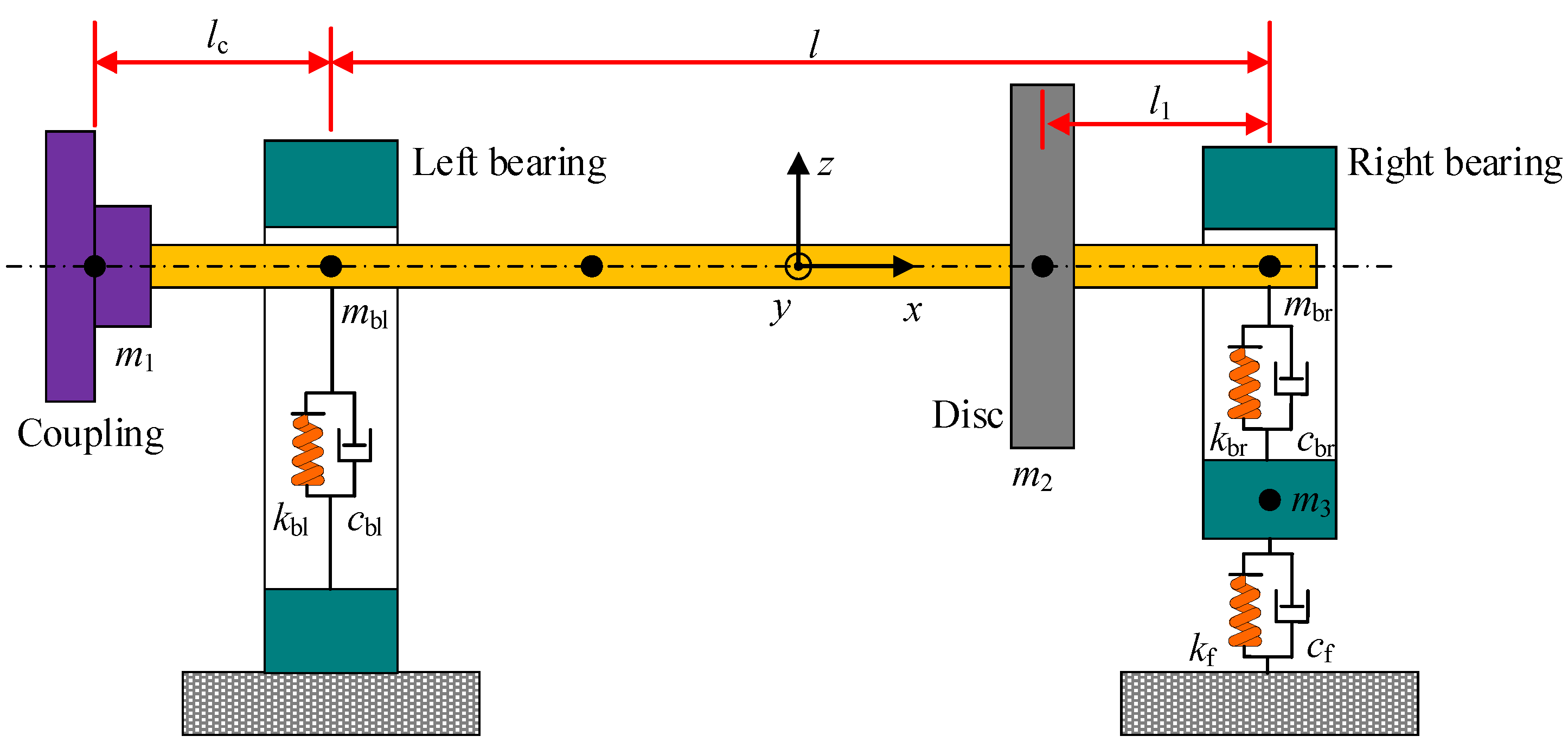
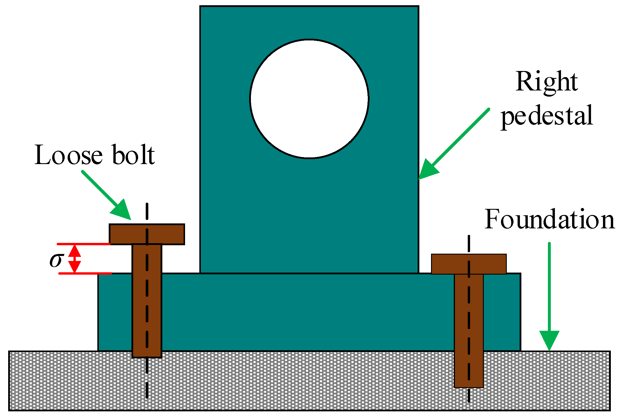
3.1. Dynamic Modelling of a Rotor-Bearing System with Pedestal Looseness

To verify the proposed fault feature extraction method, a rotor-bearing system with pedestal looseness is considered. First, based on a rotor-bearing test rig, considering the coupling structure, the finite element model of the rotor-bearing system is established, as shown in Figure 2. The specific parameters of the finite element model of the rotor-bearing system are shown in

Table 1. The specific parameters of the finite element model.

Parameters	Values
Shaft diameter at left bearing/mm	55
Shaft diameter at disc/mm	55
The span between two bearings l/mm	800
Coupling cantilever length lc/mm	165
The span between the right bearing and disc l/mm	164.5
Elastic modulus of shaft E/Pa	2.07 × 1011
Poisson’s ratio υ	0.3
Density ρ/kg/m3	7850
Horizontal and vertical stiffness of left bearing kbl/N/m	1 × 107
Horizontal and vertical damping of left bearing cbl/N·s/m	1 × 104
Horizontal and vertical stiffness of right bearing kbr/N/m	2 × 108
Horizontal and vertical damping of right bearing cbl/N·s/m	2 × 105

. The rotor structural parameters in Table 1 are consistent with the real dimensions of the test rig, while the supporting stiffness and damping are given by reference to Ref. [26] and combining the measured rotor vibration responses in the experiment.

Assume that the bearing seat at the non-driving end has a looseness fault, as shown in Figure 3. The nonlinearity caused by the looseness is simulated by a piecewise linear spring element [26,27], and the equivalent looseness stiffness is as

$$k_{\mathrm{f}}=\left\{\begin{array}{ll}{k}_{\mathrm{f}1},& z_3>\sigma \\ k_{\mathrm{f}2},& 0\le z_3\le \sigma \\ k_{\mathrm{f}3},& z_3<\sigma \end{array}\right.$$

(14)

where, k_f1 is the tensile stiffness of the bolt, k_f2 is the stiffness of the loosened bolt, k_f3 is the stiffness when the bolt is not loosened, δ is the loosening gap, and z₃ is the vibration displacement of the mass point m₃ in the z direction.

Assuming that the stiffness of the unloosed bolt is approximately equal to the tensile stiffness,

$$k_{\mathrm{f}}=\left\{\begin{array}{ll}{k}_{\mathrm{f}2},& 0\le z_3\le \sigma \\ k_{\mathrm{f}3},& \mathrm{else}\end{array}\right.$$

(15)

At this time, the governing equation of the rotor-bearing system can be expressed as

$$M\ddot{q}+D\dot{q}+Kq=Q$$

(16)

M is the mass matrix considering the mass of the shaft, coupling and disc, D is the damping matrix including bearing damping and rotor gyro moment, K is the stiffness matrix, Q is the external force vector, and q is the displacement vector.

Assume that the looseness occurs between the right bearing seat and the foundation, the looseness gap δ = 0.6 mm, the looseness mass m₃ = 12 kg, and the foundation stiffness before looseness is k_f3 = 1 × 10⁹ N/m. Assume that the eccentricity only exists at the disc, and the amount of unbalanced m·r = 880 g·mm. The rotor speed is ω = 2400 r/min, and the sampling frequency is f_s = 10,240 Hz.

This paper only considers that a single pedestal is loose, and the looseness gap is much larger than the vibration amplitude of the pedestal mass. Therefore, the change in stiffness only occurs when the pedestal is in contact with the foundation. As the degree of pedestal looseness increases, the corresponding looseness stiffness gradually decreases. The simulation mainly considers four different looseness stiffness. The stiffness of the unloose bolt is k_f3 = 1 × 10⁹ N/m, and the stiffness of the loose bolt k_f2 is 1 × 10⁹ N/m, 1 × 10⁸ N/m, 5 × 10⁷ N/m, and 1 × 10⁷ N/m. When k_f2 = 1 × 10⁹ N/m, the rotor-bearing system has no pedestal looseness fault.

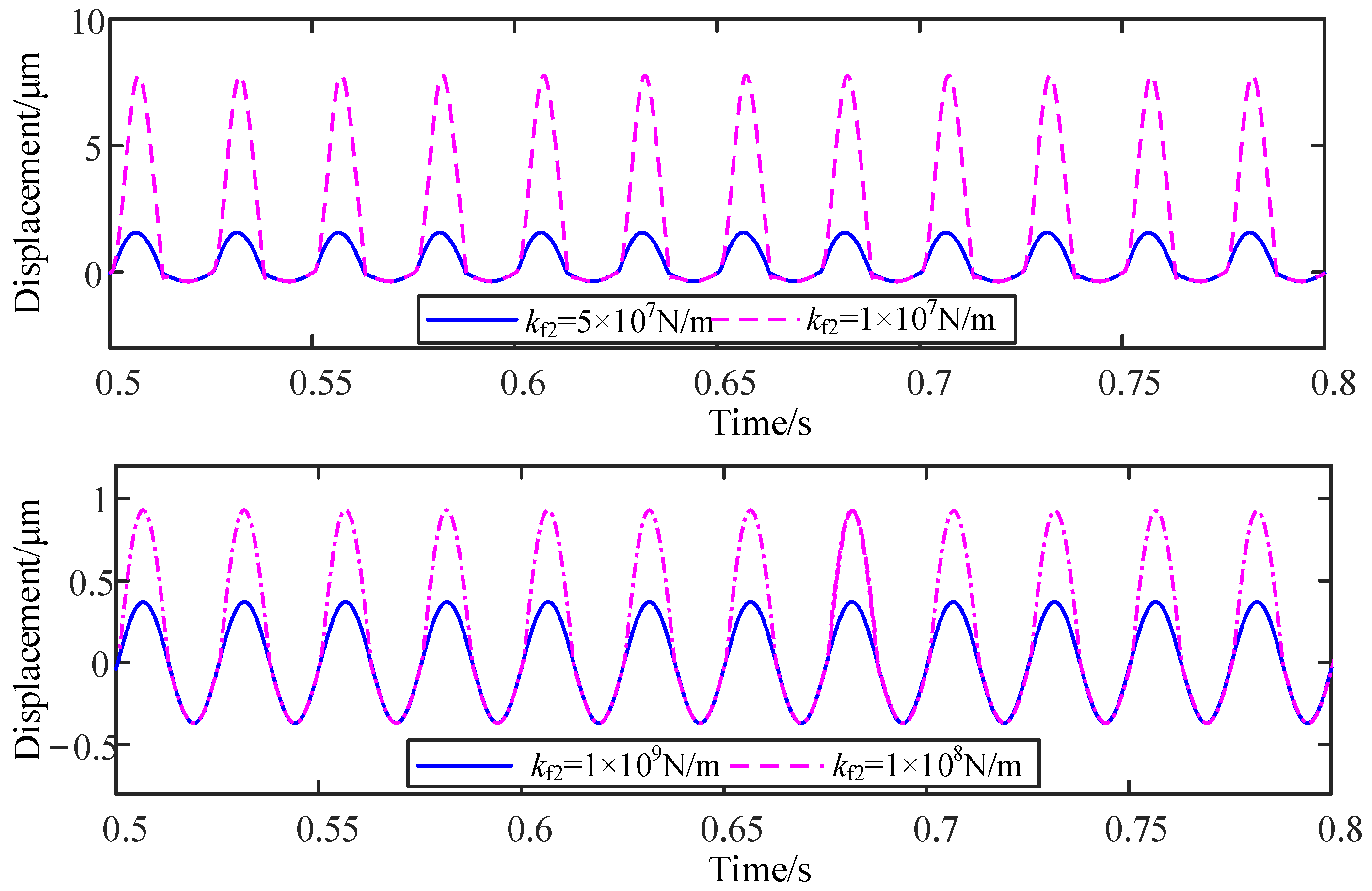
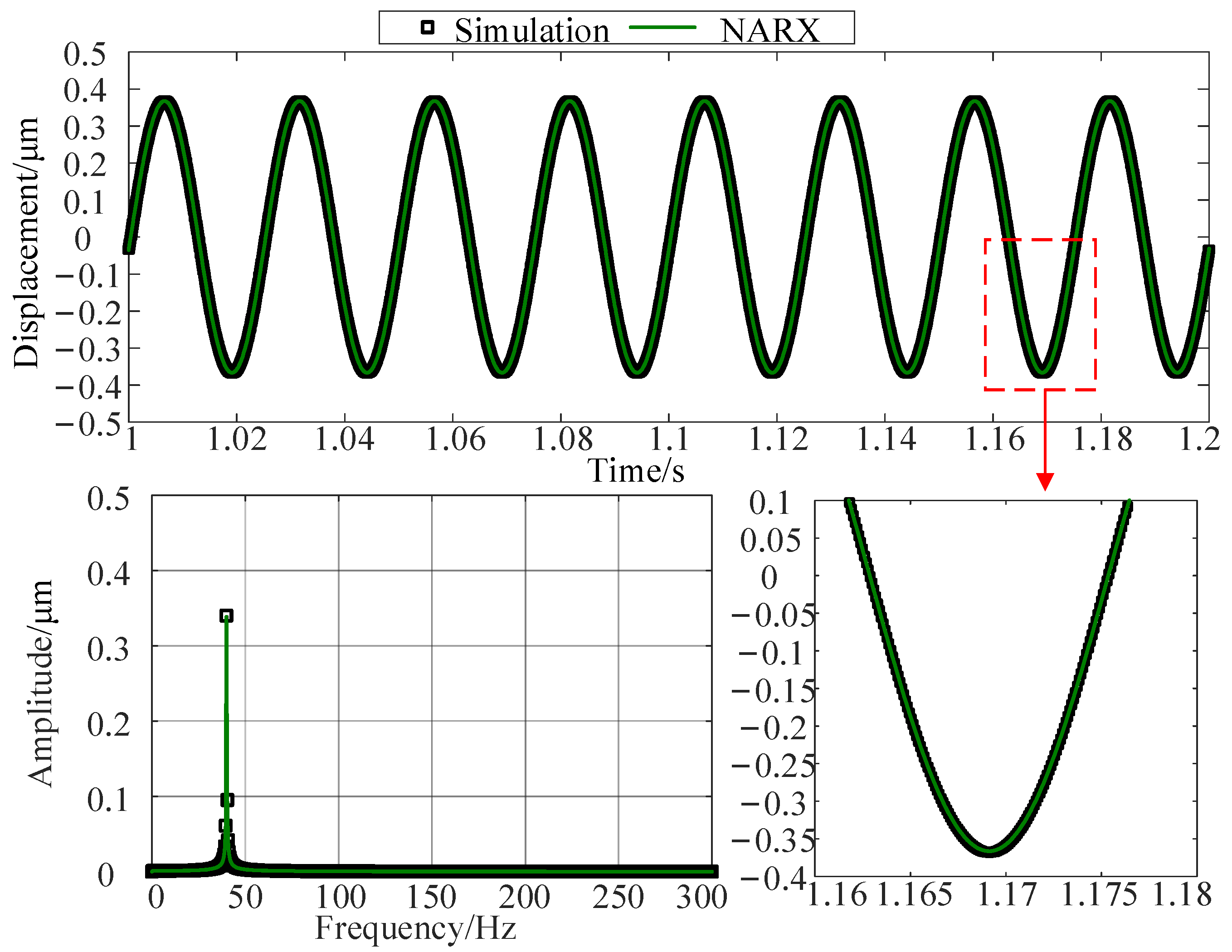
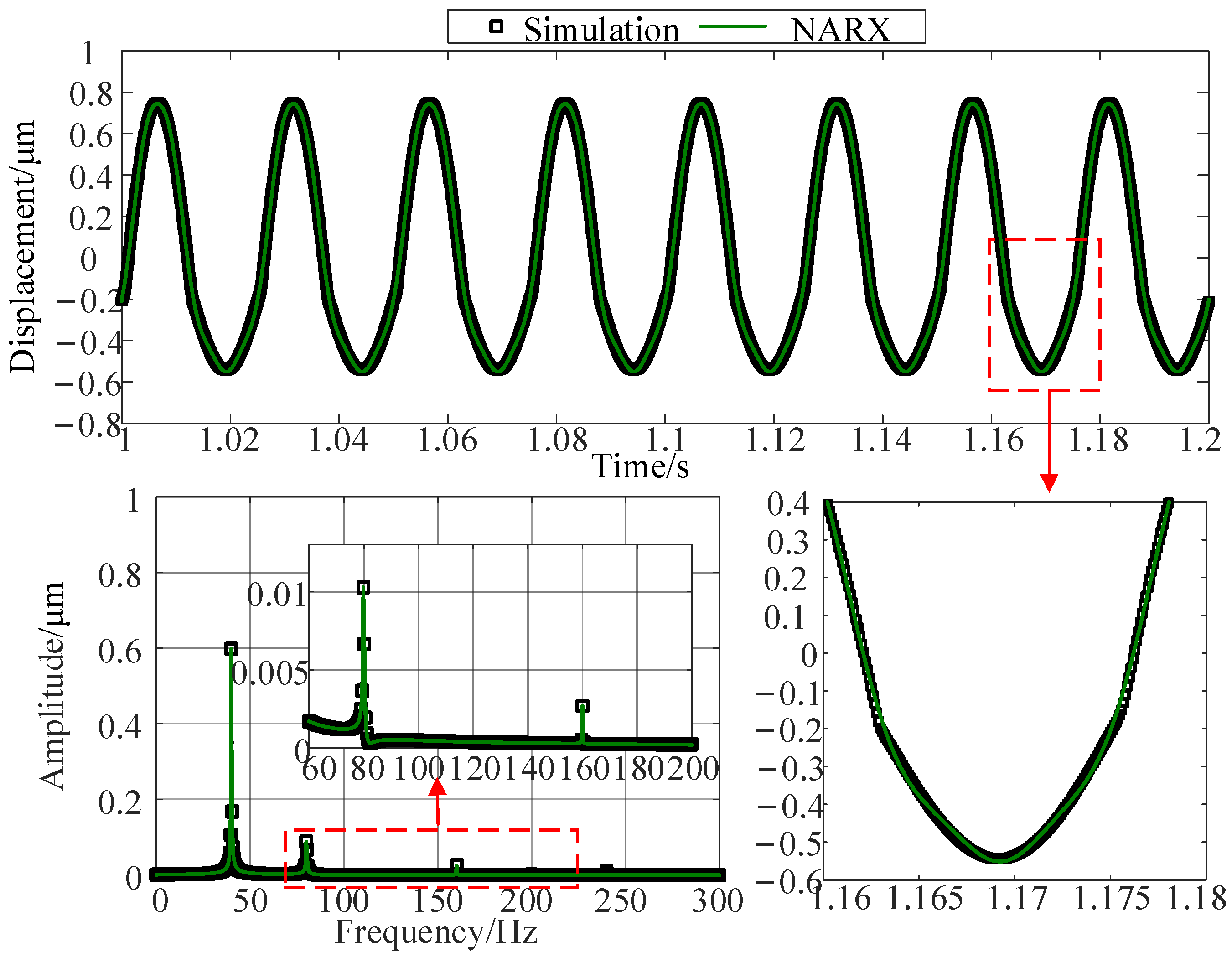
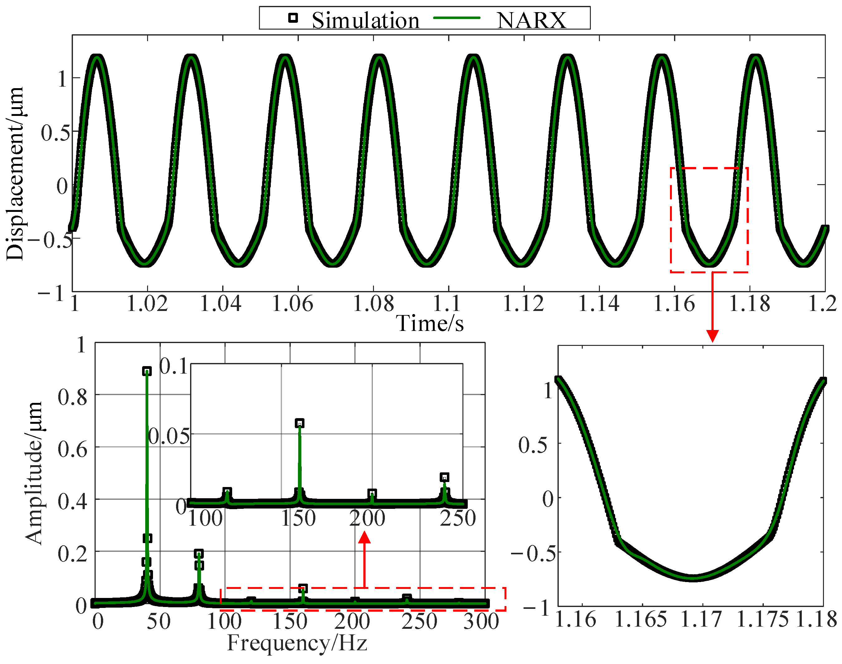
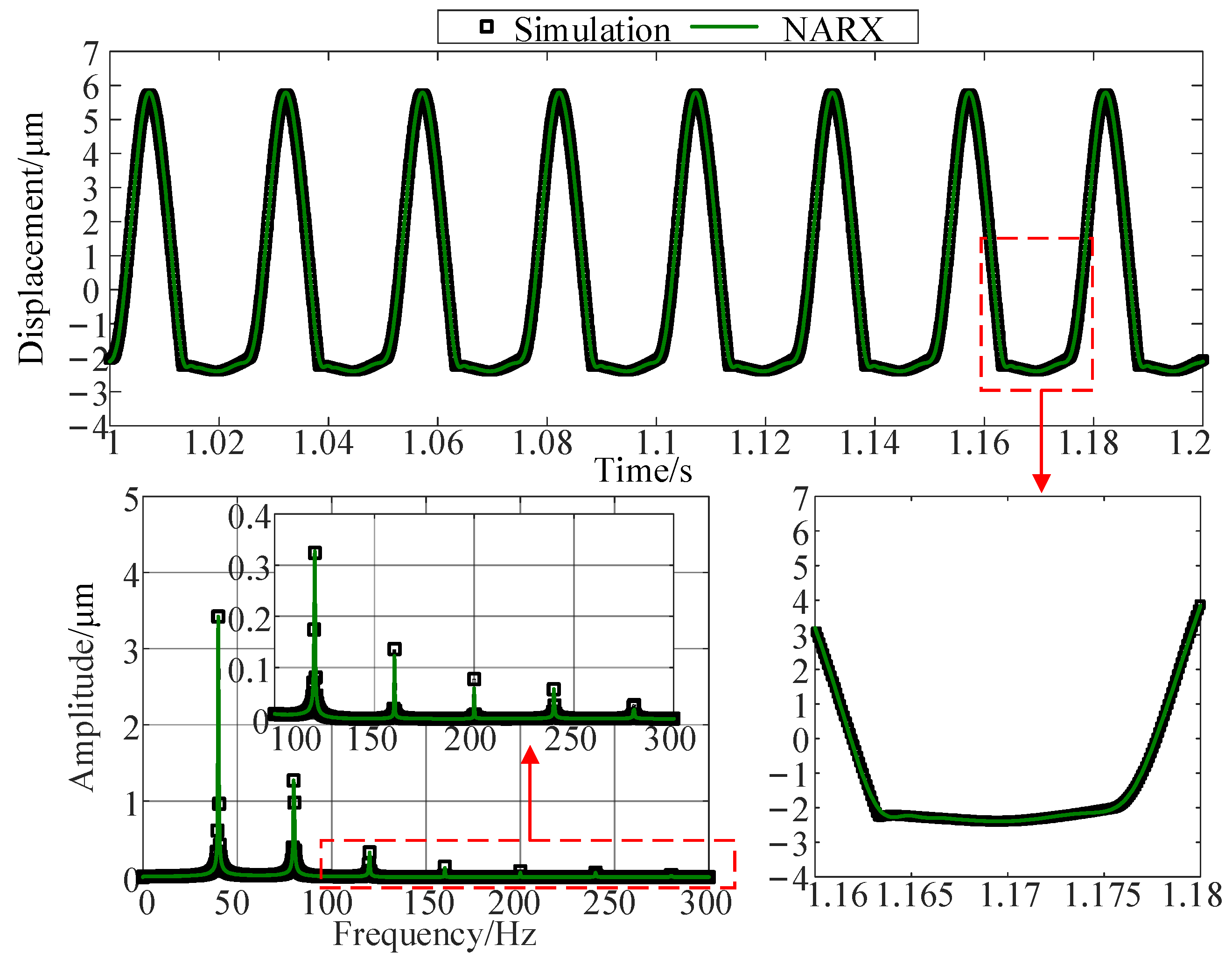
3.2. Influence of Looseness Stiffness on Vibration Response

After obtaining the differential motion equation of the rotor-bearing system, since the equation is a typical nonlinear system, the Newmark-β method is used to obtain the numerical solution. This paper mainly analyzes the influence of the looseness stiffness of the right pedestal on the vibration response, including the time domain, frequency domain, and orbit of the m_br mass point.

As the looseness stiffness decreases, the vibration amplitude of the rotating shaft gradually increases, as shown in Figure 4. The increase from 0.5 μm, when there is no looseness to the final 5 μm, is nearly ten times larger, and the increasing direction is only along the positive z-axis. This proves that the vibration amplitude is less than the looseness gap, and the pedestal can vibrate freely along the positive z-axis without restriction, which aligns with the assumption.

From the orbits in Figure 5, as the degree of looseness increases, the orbit gradually evolves from a regular ellipse when the base is not loose to an irregular ellipse with a “local cusp” and restricted on one side. It shows that a serious unilateral collision occurred in the system at this time. At the same time, from the spectrum in Figure 6, as the looseness stiffness decreases, the frequency components gradually increase. For the healthy rotor system that does not have looseness, only rotational frequency is included in the spectrum. When looseness occurs and deteriorates, namely, the looseness stiffness k_f2 gradually decreases from 1 × 10⁹ N/m to 1 × 10⁷ N/m, the amplitude of the double rotational frequency in the spectrum increases from 0 μm to 2.4125 μm. The amplitude of the double rotational frequency changes obviously, which indicates the degree of nonlinearity of the system is increasing.

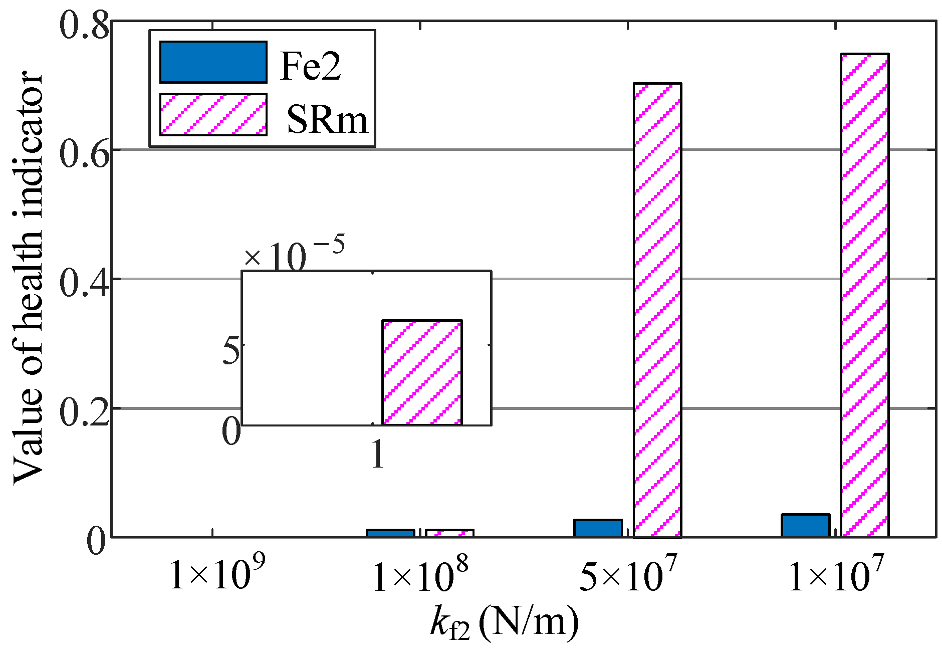
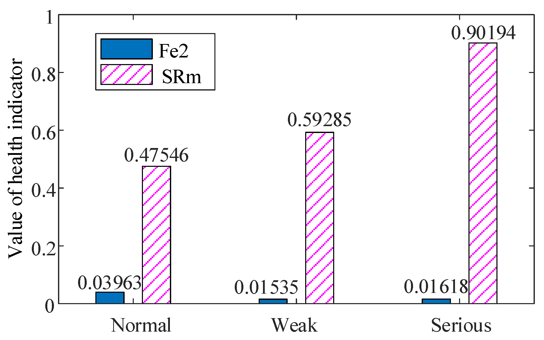
3.3. Data-Driven Fault Feature Extraction

To extract the fault feature of the pedestal looseness in the rotor-bearing system, first take the responses of m_br in z direction obtained from the numerical analysis as output, and take the synchronous excitation generated by the unbalanced force of the disc as input. Based on the FROLS method, the NARX model under different looseness stiffness is identified. Before identifying the NARX model, the initial model parameters must be determined through the trial-and-error method to make the final NARX model satisfies the MPO criterion. The number of NARX model terms is 14, and the maximum time lag of input and output is 6, respectively. The specific NARX model terms under four different looseness stiffness are shown in

Table 2. NARX model terms and coefficients under four different looseness stiffness in simulation.

No.	kf2 = 1 × 109 N/m	kf2 = 1 × 108 N/m	kf2 = 5 × 107 N/m	kf2 = 1 × 107 N/m
1	u(k − 4) [−1.81 × 10−6]	y(k − 1) [2.91]	y(k − 1) [2.84]	y(k − 1) [2.71]
2	u(k − 3) [5.21 × 10−6]	y(k − 2) [−3.77]	y(k − 2) [−3.57]	y(k − 2) [−3.37]
3	y(k − 1) [2.77]	y(k − 3) [3.27]	y(k − 3) [3.00]	y(k − 3) [2.91]
4	y(k − 2) [−2.09]	y(k − 4) [−2.31]	y(k − 4) [−2.05]	y(k − 4) [−2.09]
5	y(k − 3) [−5.32]	y(k − 5) [1.21]	y(k − 5) [9.76 × 10−1]	y(k − 5) [1.13]
6	u(k − 6) [−3.89 × 10−6]	y(k − 6) [−3.29]	y(k − 6) [−2.22 × 10−1]	y(k − 6) [−3.28]
7	y(k − 6) [−3.71 × 10−1]	u(k − 1) [1.83 × 10−2]	u(k − 1) [3.11 × 10−4]	u(k − 6) [2.33 × 10−3]
8	y(k − 5) [8.29 × 10−1]	u3(k − 1) u(k − 5) [3.78 × 10−9]	u3(k − 1)u(k − 6) [4.87 × 10−10]	u3(k − 6) [1.02 × 10−6]
9	[9.36 × 10−8]	[−3.01 × 10−3]	[−6.12 × 10−3]	[−6.58 × 10−2]
10	u(k − 2) [3.39 × 10−6]	u(k − 1)u(k − 2) [−1.31 × 10−5]	u(k − 1)u(k − 2) [4.42 × 10−6]	u(k − 1)u(k − 2)y(k − 1) [−1.91 × 10−5]
11	y(k − 4) [8.60 × 10−2]	u(k − 6) [7.26 × 10−2]	u3(k − 1) [1.46 × 10−7]	u2 (k − 6) [3.83 × 10−4]
12	u(k − 5) [−1.11 × 10−6]	u(k − 1)u(k − 3) [1.60 × 10−5]	u2(k − 1) y(k − 1) [−1.71 × 10−5]	u2(k − 5) [−3.73 × 10−4]
13	u(k − 1) [8.14 × 10−7]	u(k − 1)u2(k − 2)u(k − 4) [−4.14 × 10−9]	u(k − 1)u(k − 4)y(k − 2) [1.28 × 10−5]	u3(k − 1)y(k − 1) [1.67 × 10−7]
14	y3(k − 6) [−8.43 × 10−9]	u(k − 5) [−9.05 × 10−2]	u(k − 6)y2(k − 1) [−2.13 × 10−4]	u(k − 1)y(k − 1) [3.30 × 10−4]

. The * in [*] represents the corresponding coefficient of the terms, and the 9th line represents the constant terms.

To ensure the accuracy of the identified NARX model, the MPO prediction output of the NARX model and the actual output obtained from the numerical simulation are compared and analyzed in the time domain and frequency domain, as shown from Figure 7, Figure 8, Figure 9 and Figure 10. The predicted output of the NARX model is the same as the original simulation waveform, and the frequency domain characteristics of the first seven times the rotational frequency are consistent. It shows that the NARX model identified under each looseness stiffness has high accuracy and reliability. The effective NARX model lays the foundation for the subsequent NOFRF evaluation and further sensitive feature extraction.

After the identified NARX model has been decomposed by GALEs, the first three-order output of the system can be obtained. Combined with the first three-order input of the system, the NOFRFs can be evaluated with Equation (4). Finally, the sensitive feature indicator SRm can be obtained according to Equation (13). The comparison between SRm under different looseness stiffness and the conventional NOFRFs-based indicator Fe2 is shown in Figure 11. It can be seen that when the looseness stiffness is greater than 1 × 10⁸ N/m, the changing trend of the two indicators is the same, with the looseness stiffness decreasing. When the looseness stiffness is less than 1 × 10⁸ N/m, the indicator SRm is significantly larger than Fe2, indicating that the sensitivity of the new indicator SRm to looseness stiffness is better than that of the conventional NOFRFs-based indicator Fe2.

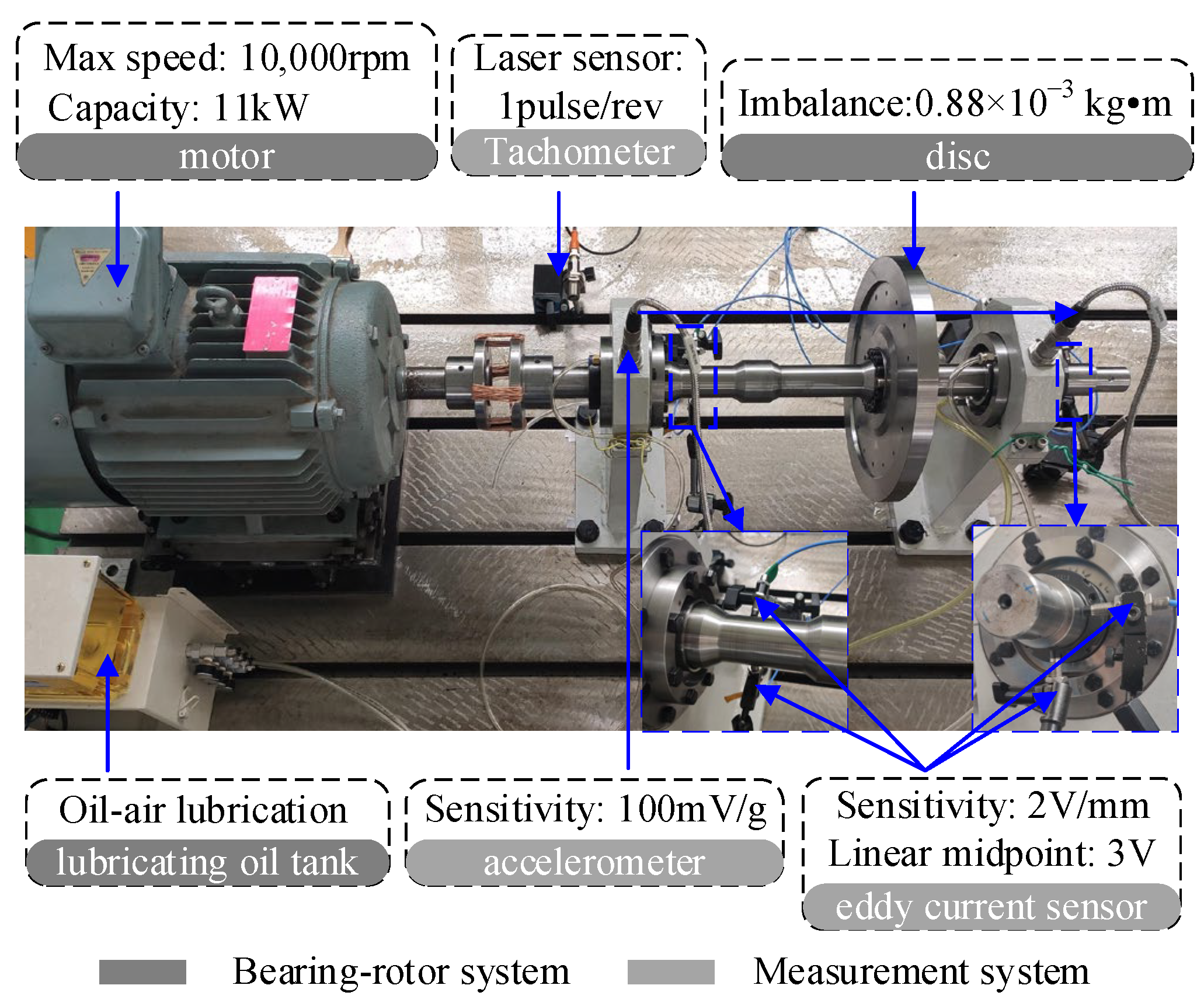
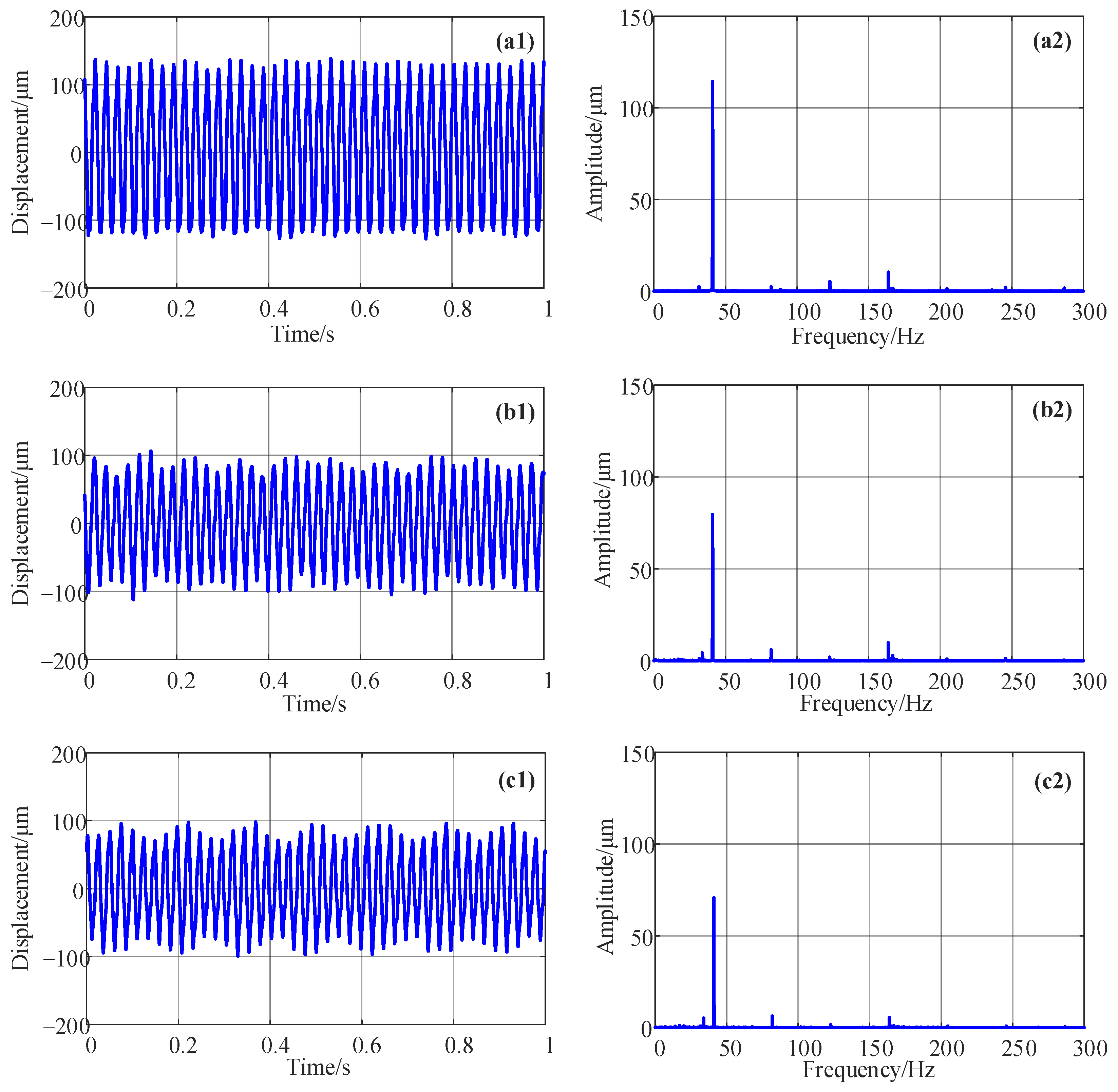
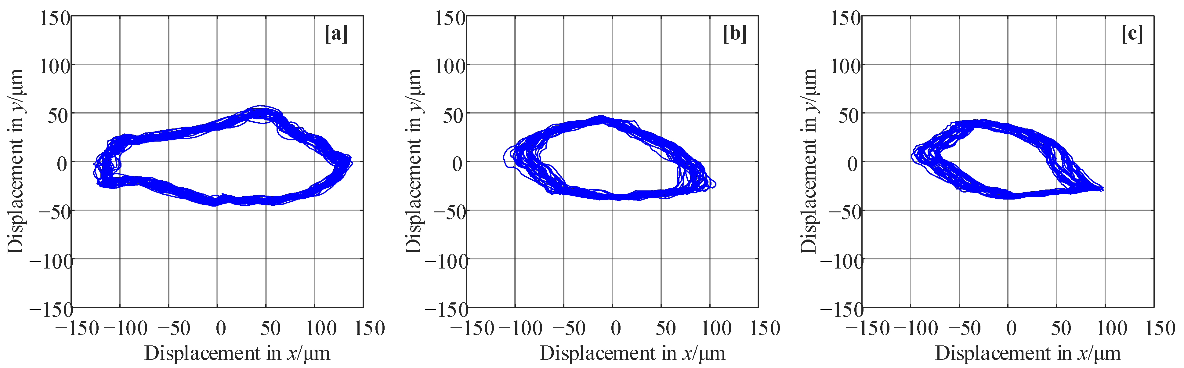
4. Experimental Verification

To verify the proposed data-driven feature extraction method and simulation results, a rotor-bearing test rig was used to analyze the influence of the pedestal looseness on the vibration response. The specific structure of the test rig is shown in Figure 12. The rotor-bearing system is a single-disc two-fulcrum structure. The test rig considers the structural characteristics of the high-pressure rotor of the aero-engine. For the high-pressure rotor, the structure has the characteristic of mass distribution bias. In addition, the support bearing of the high-pressure rotor is a cylindrical roller bearing at one end and an angular contact ball bearing at the other. The models of the two types of bearings selected for this test rig are N209E and QJ210M, respectively. The coupling is a rope coupling, which can better prevent the vibration of the motor from being transmitted to the shaft. The bearing lubrication method adopts oil-air lubrication. The pedestal at the non-driving end is loose. There are three different degrees of looseness: no looseness, slight looseness, and severe looseness.

The measurement system mainly acquires the vibration displacement signal of the shaft, the acceleration signal of the bearing seat, and the rotational speed signal. The layout of the sensors and their detailed information are shown in the dashed box in Figure 12. The eddy current sensors (model RP660677) were used to measure the vibration displacement in the horizontal and vertical directions of the shaft, respectively. The accelerometers (model BH5031EX-050-VL) were used to measure the vertical vibration acceleration of the two bearing housings at the drive and non-drive ends, respectively. A photoelectric sensor (model OGP700) was used to measure the rotational speed of the shaft through the reflective sheet pasted on the shaft. The NI-9234 card and Cdaq-9178 chassis are used to collect and store the acquired data by the self-made Labview program. The motor speed is set to 2400 rpm, and the sampling frequency f_s of the displacement and acceleration signals are both 5120 Hz.

The original horizontal vibration signal of the shaft near the non-driving end under no looseness, slight looseness, and severe looseness is shown in Figure 13. As the degree of looseness increases, the vibration amplitude decreases. The rotor–bearing test rig structure has a lot of mating gaps, and many factors affect vibration, such as assembly. When the degree of looseness increases, the vibration amplitude decreases, which may be due to the initial misalignment of the rotor system. The misalignment weakens gradually when the looseness occurs and deteriorates. This also shows that because the rotor system sometimes couples a variety of faults, the diagnosis of looseness faults simply by using changes in vibration amplitude is unreliable. Therefore, it is necessary to extract sensitive fault features to characterize looseness from the vibration signal better. From the spectrum in Figure 13, the amplitude of rotational frequency decreases, and the amplitude of double frequency increases. As the degree of looseness increases, the lower right part of the orbit becomes more and more “sharp” in Figure 14. It shows that the bearing seat collides with the foundation, consistent with the simulation results.

To effectively identify the data-driven model of the rotor-bearing test rig system and improve the accuracy of identification, the horizontal vibration signal is first comb-filtered by the Time Synchronous Averaging method to filter out noise or other frequency components that are not related to the rotational frequency. Then the vibration signal is downsampled with the downsampling frequency of 1280 Hz. Finally, the NARX models of the system in different looseness states are identified for further feature extraction. The terms and their corresponding coefficients of the NARX model under three different degrees of looseness are shown in

Table 3. NARX model terms and coefficients under three different looseness stiffness in the experiment.

No.	Normal	Weak	Serious
1	u(k − 1) [−3.58]	y(k − 1) [1.17]	u(k − 6) [−1.51 × 10−1]
2	y(k − 4) [5.24 × 10−2]	y(k − 2) [−3.58 × 10−1]	y(k − 1) [9.21 × 10−1]
3	y(k − 1) [5.96 × 10−1]	u(k − 1) [−5.61 × 10−1]	y(k − 2) [2.14 × 10−1]
4	y(k − 2) [−2.24 × 10−1]	u(k − 6)y(k − 1) [−6.66 × 10−3]	u(k − 2)u(k − 6)y(k − 2)y(k − 6) [6.34 × 10−7]
5	u(k − 2)u(k − 4)u(k − 6) [−2.08 × 10−2]	u(k − 4)y(k − 1) [9.08 × 10−3]	u(k − 1)u(k − 5)y(k − 2)y(k − 5) [−1.44 × 10−6]
6	y4(k − 6) [1.02 × 10−7]	u(k − 5)u2(k − 6)y(k − 1) [−4.73 × 10−8]	u2(k − 5)y(k − 5) [1.33 × 10−4]
7	u(k − 6)y3(k − 4) [−8.85 × 10−8]	u4(k − 6) [2.43 × 10−6]	u2(k − 1)u(k − 4) [−4.68 × 10−5]
8	y(k − 2)y(k − 6) [3.71 × 10−3]	y4(k − 1) [−3.89 × 10−7]	u(k − 3)y2(k − 2) [4.46 × 10−5]
9	y3(k − 1)y(k − 6) [9.41 × 10−8]	u(k − 1)y3(k − 1) [2.16 × 10−7]	u(k − 1)u2(k − 6)y(k − 6) [7.85 × 10−7]
10	u(k − 2)u2(k − 5) [2.07 × 10−2]	u3(k − 4) [9.76 × 10−5]	y(k − 3) [−1.91 × 10−1]
11	y(k − 3) y(k − 4)y2(k − 6) [−5.02 × 10−7]	y(k − 3)y3(k − 6) [−1.55 × 10−7]	u2(k − 2) [1.72 × 10−3]
12	u(k − 5)y2(k − 1)y(k − 4) [6.67 × 10−7]	u3(k − 1)y(k − 6) [−3.55 × 10−6]	u(k − 3)u(k − 6)y2(k − 6) [7.15 × 10−7]
13	u(k − 1)y(k − 4)y(k − 6) [8.57 × 10−5]	u(k − 5)y(k − 2)y(k − 6) [−3.84 × 10−5]	u(k − 2)u(k − 6)y(k − 4)y(k − 5) [−1.15 × 10−7]
14	y(k − 1)y2(k − 5) [2.39 × 10−6]	u(k − 3)u3(k − 6) [−2.99 × 10−6]	u(k − 3)u(k − 6)y(k − 6) [−3.52 × 10−5]
15	y(k − 1)y(k − 3)y2(k − 6) [1.72 × 10−7]	u2(k − 1)y(k − 1)y(k − 6) [−2.37 × 10−6]	u2(k − 1)u2(k − 5) [−1.62 × 10−6]
16	u(k − 4)y(k − 1)y(k − 6) [−6.14 × 10−5]	y(k − 3) [−2.14 × 10−1]	u(k − 1)u(k − 6)y(k − 2)y(k − 4) [1.94 × 10−6]
17	y2(k − 3)y(k − 5) [1.30 × 10−5]	u(k − 2)y3(k − 1) [−1.62 × 10−6]	y(k − 4) [−2.10 × 10−1]
18	u(k − 6)y(k − 3) [−3.28 × 10−3]	u2(k − 1)y(k − 5) [1.18 × 10−5]	y4(k − 3) [−2.405065 × 10−8]

.

The predicted output of the identified NARX model is compared with the experimental data processed by time synchronous averaging, as shown in Figure 15. The predicted output is highly consistent with the experimental results, which verifies the effectiveness of the NARX model under three different degrees of looseness. The identified NARX model is used to obtain the first three-order NOFRFs using the GALEs method. The second-order optimal weighted contribution rate of NOFRFs indicator SRm proposed in this paper is used to extract sensitive features and is compared with the conventional NOFRFs-based indicator Fe2. The two indicators under different looseness states are shown in Figure 16. As the degree of looseness increases, Fe2 first decreases and then increases. It is not monotonic and cannot be used to detect the change in the looseness state. The new indicator SRm showed a monotonous upward trend, increasing from 0.48 when no looseness occurs to 0.90 when severe looseness occurs, an increase of 89.7%. Therefore, the data-driven sensitive feature indicator SRm proposed in this paper can better reflect the occurrence and deterioration of system nonlinear damage.

5. Conclusions

This paper proposes a data-driven sensitive feature extraction method. First, the FROLS (Forward Regression with Orthogonal Least Squares) method is used to identify the inspected system’s NARX (Nonlinear autoregressive with exogenous inputs) model. Then the system’s NOFRFs (Nonlinear Output Frequency Response Functions) are obtained according to the GALEs (Generalized Associated Linear Equations) method. Based on the first three-order NOFRFs, the concept of the weighted contribution rate of NOFRFs is proposed, and the analytical expression of the second-order optimal weighted contribution rate of NOFRFs is derived and used as a sensitive feature. Further, the proposed method is applied to the feature extraction of the pedestal looseness of the rotor-bearing system. The dynamic model of the bearing-rotor system is established, and the piecewise linear function is used to characterize the pedestal looseness. The Newmark-β is used to solve the governing equation. Taking the unbalanced excitation of the rotor system as the input and the node response as the output, the NARX models under different degrees of looseness are identified. The model’s predicted output is compared with the numerical response, and the weighted contribution rate is used to extract the sensitive feature of looseness. Simulation results show that the sensitive feature indicator proposed in this paper is more effective than the conventional NOFRFs-based indicator. Finally, a single-disc two-fulcrum rotor-bearing test rig was established, and different degrees of pedestal looseness was simulated. The simulation analysis and the effectiveness of the proposed data-driven feature extraction method are verified. In future, the application of data-driven diagnostic methods in quantitatively analyzing faults and detecting the location of damage to engineering structures will be further explored.

References

1. Chu, F.; Tang, Y. Stability and non-linear responses of a rotor-bearing system with pedestal looseness. J. Sound Vib. 2001, 241, 879–893. [Google Scholar] [CrossRef]
2. Yang, Y.; Ouyang, H.; Yang, Y.; Cao, D.; Wang, K. Vibration analysis of a dual-rotor-bearing-double casing system with pedestal looseness and multi-stage turbine blade-casing rub. Mech. Syst. Signal Process. 2020, 143, 106845. [Google Scholar] [CrossRef]
3. Muszynska, A.; Goldman, P. Chaotic responses of unbalanced rotor/bearing/stator systems with looseness or rubs. Chaos Soliton. Fract. 1995, 5, 1683–1704. [Google Scholar] [CrossRef]
4. Jiang, M.; Wu, J.; Peng, X.; Li, X. Nonlinearity measure based assessment method for pedestal looseness of bearing-rotor systems. J. Sound Vib. 2017, 411, 232–246. [Google Scholar] [CrossRef]
5. Zhang, H.; Lu, K.; Zhang, W.; Fu, C. Investigation on dynamic behaviors of rotor system with looseness and nonlinear supporting. Mech. Syst. Signal Process. 2022, 166, 108400. [Google Scholar] [CrossRef]
6. Ma, H.; Zhao, X.; Teng, Y.; Wen, B. Analysis of dynamic characteristics for a rotor system with pedestal looseness. Shock. Vib. 2011, 18, 13–27. [Google Scholar] [CrossRef]
7. Lu, K.; Jin, Y.; Chen, Y.; Cao, Q.; Zhang, Z. Stability analysis of reduced rotor pedestal looseness fault model. Nonlinear Dyn. 2015, 82, 1611–1622. [Google Scholar] [CrossRef]
8. Yang, Y.; Yang, Y.; Cao, D.; Chen, G.; Jin, Y. Response evaluation of imbalance-rub-pedestal looseness coupling fault on a geometrically nonlinear rotor system. Mech. Syst. Signal Process. 2019, 118, 423–442. [Google Scholar] [CrossRef]
9. An, X.; Jiang, D.; Li, S.; Zhao, M. Application of the ensemble empirical mode decomposition and Hilbert transform to pedestal looseness study of direct-drive wind turbine. Energy 2011, 36, 5508–5520. [Google Scholar] [CrossRef]
10. An, X.; Zhang, F. Pedestal looseness fault diagnosis in a rotating machine based on variational mode decomposition. Proc. Inst. Mech. Eng. Part C J. Mech. Eng. Sci. 2017, 231, 2493–2502. [Google Scholar] [CrossRef]
11. Lee, S.M.; Choi, Y.S. Fault diagnosis of partial rub and looseness in rotating machinery using Hilbert-Huang transform. J. Mech. Sci. Technol. 2008, 22, 2151–2162. [Google Scholar] [CrossRef]
12. Billings, S.A. Nonlinear System Identification: NARMAX Methods in the Time, Frequency, and Spatio-Temporal Domains; John Wiley & Sons: Hoboken, NJ, USA, 2013. [Google Scholar]
13. Junsheng, C.; Dejie, Y.; Yu, Y. A fault diagnosis approach for roller bearings based on EMD method and AR model. Mech. Syst. Signal Process. 2006, 20, 350–362. [Google Scholar] [CrossRef]
14. McLeod, A.I.; Li, W.K. Diagnostic checking ARMA time series models using squared-residual autocorrelations. J. Time Ser. Anal. 1983, 4, 269–273. [Google Scholar] [CrossRef]
15. Doyle III, F.J.; Ogunnaike, B.A.; Pearson, R.K. Nonlinear model-based control using second-order Volterra models. Automatica 1995, 31, 697–714. [Google Scholar] [CrossRef]
16. Ding, F.; Liu, X.P.; Liu, G. Identification methods for Hammerstein nonlinear systems. Digit. Signal Process. 2011, 21, 215–238. [Google Scholar] [CrossRef]
17. Chen, S.; Billings, S.A. Representations of non-linear systems: The NARMAX model. Int. J. Control 1989, 49, 1013–1032. [Google Scholar] [CrossRef]
18. Karami, K.; Westwick, D.; Schoukens, J. Applying polynomial decoupling methods to the polynomial NARX model. Mech. Syst. Signal Process. 2021, 148, 107134. [Google Scholar] [CrossRef]
19. Zhang, S.; Lang, Z.Q. SCADA-data-based wind turbine fault detection: A dynamic model sensor method. Control Eng. Pract. 2020, 102, 104546. [Google Scholar] [CrossRef]
20. Zhu, Y.P.; Lang, Z.Q.; Mao, H.L.; Laalej, H. Nonlinear output frequency response functions: A new evaluation approach and applications to railway and manufacturing systems’ condition monitoring. Mech. Syst. Signal Process. 2022, 163, 108179. [Google Scholar] [CrossRef]
21. Li, Y.; Luo, Z.; He, F.; Zhu, Y.; Ge, X. Modeling of rotating machinery: A novel frequency sweep system identification approach. J. Sound Vib. 2021, 494, 115882. [Google Scholar] [CrossRef]
22. Lang, Z.Q.; Billings, S.A.; Yue, R.; Li, J. Output frequency response function of nonlinear Volterra systems. Automatica 2007, 43, 805–816. [Google Scholar] [CrossRef]
23. Liu, Y.; Zhao, Y.L.; Li, J.T.; Ma, H.; Yang, Q.; Yan, X.X. Application of weighted contribution rate of nonlinear output frequency response functions to rotor rub-impact. Mech. Syst. Signal Process. 2020, 136, 106518. [Google Scholar] [CrossRef]
24. Zhao, Y.; Zhu, Y.P.; Han, Q.; Liu, Y. The evaluation of Nonlinear Output Frequency Response Functions based on tailored data-driven modelling for rotor condition monitoring. Mech. Syst. Signal Process. 2023, 197, 110409. [Google Scholar] [CrossRef]
25. Peng, Z.K.; Lang, Z.Q.; Wolters, C.; Billings, S.A.; Worden, K. Feasibility study of structural damage detection using NARMAX modelling and nonlinear output frequency response function based analysis. Mech. Syst. Signal Process. 2011, 25, 1045–1061. [Google Scholar] [CrossRef]
26. Lin, J.; Zhao, Y.; Wang, P.; Wang, Y.; Han, Q.; Ma, H. Nonlinear Responses of a Rotor-Bearing-Seal System with Pedestal Looseness. Shock. Vib. 2021, 2021, 9937700. [Google Scholar] [CrossRef]
27. Choi, S.K.; Noah, S.T. Response and stability analysis of piecewise-linear oscillators under multi-forcing frequencies. Nonlinear Dyn. 1992, 3, 105–121. [Google Scholar] [CrossRef]
Figure 1. The data-driven sensitive feature extraction process.
Mathematics 11 02769 g001
Figure 2. Mechanical model of a rotor-bearing system.
Mathematics 11 02769 g002
Figure 3. Bolt looseness schematic.
Mathematics 11 02769 g003
Figure 4. Vibration responses when kf2 = 1 × 10⁹ N/m, 1 × 10⁸ N/m, 5 × 10⁷ N/m, and 1 × 10⁷ N/m.
Mathematics 11 02769 g004
Figure 5. Orbits when kf2 = 1 × 10⁹ N/m, 1 × 10⁸ N/m, 5 × 10⁷ N/m, and 1 × 10⁷ N/m.
Mathematics 11 02769 g005
Figure 6. Spectrum when kf2 = (a) 1 × 10⁹ N/m (b) 1 × 10⁸ N/m (c) 5 × 10⁷ N/m (d) 1 × 10⁷ N/m.
Mathematics 11 02769 g006
Figure 7. NARX model predicted output when kf2 = 1 × 10⁹ N/m.
Mathematics 11 02769 g007
Figure 8. NARX model predicted output when kf2 = 1 × 10⁸ N/m.
Mathematics 11 02769 g008
Figure 9. NARX model predicted output when kf2 = 5 × 10⁷ N/m.
Mathematics 11 02769 g009
Figure 10. NARX model predicted output when kf2 = 1 × 10⁷ N/m.
Mathematics 11 02769 g010
Figure 11. The changing trend of the health indicator SRm with looseness stiffness.
Mathematics 11 02769 g011
Figure 12. Test rig structure and sensors installation location.
Mathematics 11 02769 g012
Figure 13. Vibration waveform and spectrum at the non-driving end (a1,a2) No looseness (b1,b2) Slight looseness (c1,c2) Severe looseness.
Mathematics 11 02769 g013
Figure 14. Shaft orbit at the non-driving end (a) No looseness (b) Slight looseness (c) Severe looseness.
Mathematics 11 02769 g014
Figure 15. NARX model prediction output (a) No looseness (b) Slight looseness (c) Severe looseness.
Mathematics 11 02769 g015
Figure 16. Hearth indicator values under three different degrees of looseness.
Mathematics 11 02769 g016