Article

A Distributed Optimization Accelerated Algorithm with Uncoordinated Time-Varying Step-Sizes in an Undirected Network

1
Database and Artificial Intelligence Laboratory, College of Computer and Information Science, Southwest University, Chongqing 400715, China
2
College of Big Data and Software, Chongqing College of Mobile Communication, Chongqing 401520, China
3
Business College, Southwest University, Chongqing 402460, China
*
Author to whom correspondence should be addressed.
Mathematics 2022, 10(3), 357; https://doi.org/10.3390/math10030357
Submission received: 12 December 2021 / Revised: 14 January 2022 / Accepted: 21 January 2022 / Published: 25 January 2022
(This article belongs to the Special Issue Modeling and Analysis of Complex Networks)

Abstract

:
In recent years, significant progress has been made in the field of distributed optimization algorithms. This study focused on the distributed convex optimization problem over an undirected network. The target was to minimize the average of all local objective functions known by each agent while each agent communicates necessary information only with its neighbors. Based on the state-of-the-art algorithm, we proposed a novel distributed optimization algorithm, when the objective function of each agent satisfies smoothness and strong convexity. Faster convergence can be attained by utilizing Nesterov and Heavy-ball accelerated methods simultaneously, making the algorithm widely applicable to many large-scale distributed tasks. Meanwhile, the step-sizes and accelerated momentum coefficients are designed as uncoordinate, time-varying, and nonidentical, which can make the algorithm adapt to a wide range of application scenarios. Under some necessary assumptions and conditions, through rigorous theoretical analysis, a linear convergence rate was achieved. Finally, the numerical experiments over a real dataset demonstrate the superiority and efficacy of the novel algorithm compared to similar algorithms.

1. Introduction

In recent years, with the rapid development of artificial intelligence, big data, etc., there has been much attention to distributed optimization problems in multi-agent systems. As one of the most important fields, distributed optimization methods have gained significant growing interest due to the widespread applications in science and engineering areas such as the transmission of information in wireless sensor networks [1,2,3], the collaboration of vehicles in formation control [4,5], speeding up the optimization process in distributed machine learning [6,7], distributed resource allocation in smart-grid networks [8,9,10], distributed control in nonlinear dynamical systems [11,12], etc. Specifically, a distributed optimization framework can avoid the establishment of long-distance communication between agents while providing better load balancing for the network. Compared to traditional centralized optimization, agents in a multi-agent system communicate information only with their neighbors for distributed optimization. At the same time, the local objective function of each agent is known only by itself.
Literature Review: Since the DGD (Distributed gradient descent) algorithm was proposed by Nedic [13] for solving distributed convex problem in multiagent systems, great progress has been made in the distributed optimization field. Especially, the distributed first-order methods have attracted many researchers’ attention. Based on consensus theory [14] and gradient-descent technology, diminishing step-sizes were introduced into the algorithm DGD [13], which made the algorithm converge to the exact optimal solution but with a sublinear rate. When there were constraints of a decision variable, by utilizing the projection method, Sundhar [15] proposed a stochastic subgradient projection algorithm. Similar to [13,15], refs. [16,17,18] also employed the diminishing step-sizes, and these algorithms could converge linearly. However, diminishing step-sizes will lead to a much slower convergence rate. Then, the distributed algorithms with constant step-sizes were developed in [19,20,21,22,23,24,25,26,27,28,29,30,31,32] to overcome the shortcoming. The algorithm EXTRA [19] (Extra: An exact first-order algorithm for decentralized consensus optimization) and its improvement [20,21,22] modified the update rule of DGD by taking the difference of two consecutive iterations of formulas. Compared to DGD, the linear convergence rate can be verified in EXTRA, and even the step-size was fixed to a constant; EXTRA was more stable, but two weight matrices in EXTRA must obey strict conditions called the Mixing Matrix. A different type of distributed optimization algorithm HSADO (harnessing smoothness to accelerate distributed optimization) was proposed by Qu and Li [26] when the local objective functions were convex and smooth. HSADO adopted a gradient-tracking mechanism, which replaced the gradient term in DGD with a tracking gradient that was the gradient estimation of the average gradient of the whole network. If the step-sizes were set to constants, HSADO also can converge to the optimal solution linearly. Based on HSADO, researchers modified to adapt different scenarios, such as time-varying networks [27,28] and node-varying [29,30] and accelerated methods [31,32]. Further, researchers studied the primal-dual method in distributed optimization by utilizing the Augmented Lagrangian function; the original problem was reformulated in a dual problem. It has been demonstrated that EXTRA was equivalent to the algorithms in  [33,34] by introducing dual variables, and  [27] also provided a primal-dual interpretation for HSADO. Recently, the primal-dual algorithm UG (A unification and generalization of exact distributed first-order methods) proposed in [35] unified and generalized the methods EXTRA and HSADO, while it also converged linearly.
Motivations: Among these studies, EXTRA, HSADO, and UG are most related to our research. The algorithm UG can be regard as a generalization and unification of DGD, EXTRA, and HSADO. However, each local objective function of the agent in the network requires to be twice continuously differentiable, which is a rigorous condition in actual scenarios. In order to obtain linear convergence, fixed constant step-sizes were frequently adopted in distributed optimization algorithms such as  [19,26,35], etc. Unfortunately, uncoordinated step-sizes for different agents are required rather than the same constant step-sizes. This situation was first studied in  [36], in which an augmented distributed-gradient method was proposed, but it converged sublinearly. Then, by employing uncoordinated step-sizes, Lü [30] and Jakovetic [28] both established a global linear convergence of their algorithms in time-varying undirected and directed networks, respectively. To endow more independence, time-varying and nonidentical step-sizes of each agent were studied. A primal-dual fixed-point algorithm with nonidentical step-sizes was proposed by Li [37] when the object function of each agent was twice differentiable and nonsmooth. Xin  [32] also adopted nonidentical step-sizes in a directed network. With a more relaxed step-size and network topolog, a distributed primal-dual optimization method in  [38] was proposed by utilizing time-varying step-sizes, which was proved to converge linearly. Until now, to the best knowledge of the authors, no related studies for the widely used algorithm UG with uncoordinated, time-varying, and nonidentical step-sizes in an undirected network were studied. Recently, as optimization processes of large-scale tasks such as deep learning are getting slower, the convergence rate of distributed optimization algorithms need further improvement. With the help of Nesterov [39] and Heavy-ball [40] accelerated methods, the convergence rate of distributed optimization algorithms can be improved. In [32], a Heavy-ball distributed accelerated method with gradient-tracking technology was proposed to accelerate the well-known row-stochastic and column-stochastic algorithm [41]. In [31,42], a better convergence rate was shown by utilizing the Nesterov accelerated method. Moreover, both the Heavy-ball and Nesterov accelerated methods were introduced to improve the convergence rate in directed networks for machine learning in  [43]. For the widely used algorithm UG, it is challenging to study whether the simultaneous inclusion of Heavy-ball and Nesterov momentum can bring about a faster convergence rate in large-scale computing and communication tasks.
Statement of Contributions: Throughout this article, we mainly focus on the application of distributed convex optimization method over an undirected network. We propose a novel distributed optimization algorithm with uncoordinated, time-varying, and nonidentical step-sizes and accelerated momentum terms, which has a faster linear convergence rate and can apply to more scenarios. To summarize, three contributions are as follows:
  • Based on the distributed optimization methods [19,26,35], we designed and discussed a faster distributed optimization accelerated algorithm, named UGNH (UG with Nesterov and Heavy-ball accelerated methods), which solves the distributed convex problems over an undirected network. In particular, the momentum with the Nesterov and Heavy-ball methods together improve the convergence rate, which can be seen in the numerical experiments.
  • Compared to related algorithms, in our algorithm, not only the step-sizes but the coefficients of momentum terms (for convenience, we call them coefficients for short later) are uncoordinated, time-varying, and nonidentical, which are locally chosen for each agent. Through convergence analysis, the step-sizes and coefficients are more flexible than most existing methods. Meanwhile, if the local objective functions satisfy the conditions that are smooth and strongly convex, we can obtain an upper bound of step-sizes and coefficients. Under the upper bounds, the sequences generated by UGNH converge to the exact optimal solutions linearly.
  • In contrast to related algorithms, the upper bounds of the largest step-sizes and coefficients of UGNH are more relaxed, which only depend on the parameters of objective functions and the topology of the network. Meanwhile, there can be zero step-sizes and coefficients (not all) among agents.
Organization: The rest of this article is arranged as follows. In Section 2, we describe the distributed problem and provide some necessary assumptions. In Section 3, we discuss the development of relevant distributed optimization algorithms and two classical accelerated methods and then propose a new distributed accelerated algorithm. Convergence analysis is detailed in Section 4. In Section 5, numerical experiments are provided to demonstrate the superiority and efficiency of our algorithm. Finally, Section 6 concludes this article and provides some research directions for the future.
Basic Notation: Throughout the rest of this article, unless otherwise specified, all vectors are considered as column vectors, and n is the number of agents in network. The real-number set, the natural-number set, and the m-dimensional real column vector are denoted by R , N , and R m , respectively. The subscript notations i , j 1 , 2 , , n represent the indices of the agents, while the superscript notation t represents an index for the iteration step, e.g., x i t represents the ith agent’s decision variable at the jth iteration; 0 n R n , 1 n R n , and I n R n × n denote an n-dimensional zero vector, one vector, and an identity matrix, respectively. For a matrix P, p i j denotes the element at the i-th row and the j-th column of P, while its spectral radius and spectral norm are defined as ρ P and P , respectively. Similarly, x denotes the 2-norm for vector x. The transpose of a vector x and a matrix P are denoted by x T and P T , respectively. For a vector r = r 1 , r 2 , , r n T , diag(r) represents a diagonal matrix, the diagonal elements of which equal to the vector r. The notation ⊗ represents the Kronecker product. Let f x : R m R m denote the gradient of f x at x.

2. Preliminaries

This section describes the formulation of the distributed optimization problem and some necessary basic assumptions related to network and function.

2.1. Problem Formulation

Consider an undirected network of n agents, which cooperatively solve the optimization problem written in the following form over a common variable x R m :
min x R m f x = 1 n i = 1 n f i x
Here, each local objective function f i : R m R with a convex property is possessed by agent i, which exchanges local information only with its neighbors. Our main target was to design a distributed optimization algorithm, a decision variable of which can linearly converge to the optimal solution that minimizes the average of all local objective functions. The optimal average objective value of problem (1) is defined as f x ˜ * , where x ˜ * R m is the optimal decision variable. Then, the global optimal solution of (1) is denoted by x * R n m , where x * = 1 n x ˜ * .
As a local copy of the global decision variable is saved at each agent, optimization problem (1) can be solved in a distributed way by iterating the decision variable. In this study, network is described as G = V , E , where V = 1 , 2 , , n is the vertex set that represents the agents of the network, and E = i , j | i , j V is the edges set. In an undirected network, an edge i , j E implies that an edge j , i E too. Meanwhile, agent i and agent j can exchange information with each other. Let N i = j | i , j E i denote the set of all neighbors of agent i. Then, formulation (1) can be rewritten as follows:
min x R n m f x = 1 n i = 1 n f i x i
where x = x 1 T , x 2 T , , x n T T R n m , x i = x j for i , j V . Recently, it has been proved that a new equality 1 α L 1 2 x = 0 is equivalent to the consensus condition x i = x j in  [33], where α is the step-size, and L = I P is a Laplace matrix. Then, the primal-dual method can be introduced to solve (2) by utilizing the Augmented Lagrangian function, which is also a cornerstone of our algorithm.
Next, some necessary assumptions about the underlying graph and local objective functions are formalized, which are a common standard in related distributed optimization studies.

2.2. Assumptions

Assumption 1
([35]). The network G = V , E is connected, undirected, and simple. In particular, there are no self-loops of any agent and no multiple links between any two agents.
Assumption 2
([19]). A non-negative symmetric doubly stochastic weight matrix P = p i j R n × n is defined to represent network G . The weight of the matrix P satisfies the following three conditions:
  • Non-negative: p i j = > 0 , j N i = 0 , o t h e r w i s e
  • Symmetric: p i j = p j i
  • Doubly stochastic: i = 1 n p i j = j = 1 n p i j = 1
Assumption 3.
Each local objective function f i : R m R , i V is smooth with Lipschitz constant ψ i and strongly convex with parameter μ i . Mathematically, there exits ψ i > 0 , μ i 0 μ i > 0 , for any x , y R m such that:
f i x f i y ψ i x y f i x f i y f i x T x y + μ i 2 x y
Remark 1.
Assumption 1 ensures that each agent can directly or indirectly affect other agents in the network. Assumption 3 is a standard assumption in convergence analysis of distributed optimization methods. Especially, under the assumption of strongly convex for each function, there exists a unique global optimal solution to problem (1). Moreover, for the global objective function f, we define ψ ¯ = 1 n i = 1 n ψ i as the global Lipschitz constant and μ ¯ = 1 n i = 1 n μ i as the global strongly convex parameter.

3. Algorithm Development

In this section, Section 3.1 describes the development of some related algorithms. Section 3.2 describes the Nesterov and Heavy-ball accelerated methods for the distributed optimization algorithm. Section 3.3 describes the proposed algorithm UGNH and the relationship between UGNH and the previous algorithms.

3.1. Related Algorithms

In this subsection, we focus on some classical algorithms DGD, EXTRA, HSADO, and UG, which are related to the proposed algorithm and give them a simple explanation.
In  [13], Nedic and Ozdaglar proposed a standard distributed gradient descent method DGD. The method updated the decision variable at each agent through its neighbors and the local negative gradient’s direction, as follows:
x i t + 1 = j N i p i j x j t α t f i x i t
where α t was the step-size, which satisfied α t > 0 , t = 0 α t = , and α t 2 < ; the matrix P satisfied Assumption 2. The variable x i t stored in the agents is the local estimate of x at the t-th iteration. It was proved that sequences generated by DGD cannot converge to the exact optimal solution x * when employing a fixed step-size, i.e., α t = α . By taking an appropriately diminishing step-sizes, DGD can converge accurately, but the convergence rate was sublinear.
To acquire linear convergence, Shi [19] proposed a new method EXTRA by modifying the update rule of DGD (3). There were two steps performed as follows:
x i 1 = j N i p i j x j 0 α f i x i 0 ( 4 ) x i t + 1 = x i t + j N i p i j x j t j N i p ˜ i j x j t 1 α f i x i t f i x i t 1 ( 5 )
where the step-size α > 0 was a constant, the matrix P satisfied Assumption 2, while P ˜ = I + P 2 was appropriate. Compared to DGD (3), an initial condition (4) and one more iteration (5) were added. Notably, the step-size was a constant, but EXTRA can linearly converge to the exact optimal solution as long as the step-size was chosen appropriately.
Based on DGD (3), Qu and Li [26] proposed a novel distributed algorithm HSADO by using gradient-tracking technology. An auxiliary variable z i t was introduced to estimate the network-wide gradient average 1 n i = 1 n f i x i t at the t-th iteration for agent i. As a result, the gradient contribution α f i x i t in (3) was replaced by α z i t . The specific updating rules were as follows:
x i t + 1 = j N i p i j x j t α z i t ( 6 ) z i t + 1 = j N i p i j z j t + f i x i t + 1 f i x i t ( 7 )
where the step-size α > 0 was a constant, and the matrix P satisfied Assumption 2. Under the previous assumptions, initialized with x i 0 R m and z i 0 = f i x i 0 , a global linear convergence rate could be gained when choosing an appropriate fixed step-size.
Recently, a novel distributed optimization algorithm UG was proposed in [35], which used the primal-dual method to solve the equivalent problem (2). Through tuning parameters, the algorithm subsumed the well-known algorithm EXTRA and HSADO. Updating rules were as follows:    
x i t + 1 = j N i p i j x j t α f i x i t + z i t ( 8 ) z i t + 1 = z i t j N i l i j f j x j t + z j t q N j k j q x q t ( 9 )
where the step-size α > 0 was a constant; x i t was primal variable; and z i t was dual variable, which were initialized to x i 0 R m and z i 0 = 0 m , respectively. For using more-compact notation, we defined P = p i j , L = l i j , and K = k i j . The matrix L = I n P and the matrix K R n × n are symmetric with the property that there exists some constant λ such that K 1 n = λ 1 n .
By analyzing when the matrix K is chosen properly, the algorithm UG is equivalent to: (1) EXTRA, when K = 1 α P and (2) HSADO, when K = 0 n . For others, K = μ ¯ + ψ ¯ 2 I n and K = μ ¯ + ψ ¯ 1 + λ n P ( λ n is the smallest eigenvalue of matrix P) are appropriate for K = k I n and K = k P , respectively. There are no extra computational variables and no communication relationships with other agents in the formula K , so (8) and (9) are easy to implement. As UG unifies and generalizes previous methods, we mainly focused on it.

3.2. Distributed Accelerated Methods

In this section, centralized Nesterov and Heavy-ball accelerated methods will be introduced. With them, many distributed optimization algorithms can converge faster.
For the gradient-descent algorithm, i.e., x i t + 1 = x i t α f i x i t , the best achievable convergence is O κ 1 κ + 1 t ; κ = ψ ¯ μ ¯ denotes the condition number of the objective function. If ψ ¯ is much larger than μ ¯ so that κ is large, then the gradient descent becomes quite slow. To accelerate the gradient descent, Polyak [40] proposed a method called Heavy-ball for updating decision variable. The specifics was as follows:
x i t + 1 = x i t α f i x i t + γ x i t x i t 1
where γ was the momentum-accelerated coefficient, and the term γ x i t x i t 1 was used to accelerate the convergence of the decision variable. It had been proved that under the appropriate step-size α and the coefficient γ , the momentum-accelerated method could achieve a convergence rate of O κ 1 κ + 1 t , which was obviously faster.
Inspired by conjugate gradient methods [44], history gradient information can improve the convergence rate for distributed first-order optimization algorithms. Nesterov proposed a method called CNGD [40] (Centralised Nesterov Gradient Descent method) as follows:
x i t + 1 = y i t α f i y i t ( 11 ) y i t + 1 = x i t + 1 + γ x i t + 1 x i t ( 12 )
where α = μ ¯ ψ ¯ , γ = ψ ¯ μ ¯ ψ ¯ + μ ¯ . It had been proved that CNGD achieved the best convergence rate among all centralized gradient methods within first-order algorithms. Under the previous assumptions, CNGD achieved a faster convergence rate O 1 μ ¯ ψ ¯ t , compared to the CGD’s convergence rate O 1 μ ¯ ψ ¯ t .
It is notable that the two accelerated methods have been adapted in many distributed algorithms, such as  [42,43], etc. In this study, we devoted ourselves to studying the two accelerated methods on UG.

3.3. The Proposed Algorithm

The recent studies  [35,42] are the most relevant to our work. Based on these works, considering that the Nesterov and Heavy-ball accelerated methods are very helpful for achieving a faster convergence, we added them into UG simultaneously. Meanwhile, in order to apply in many more scenarios, the step-sizes and coefficients were designed as uncoordinated, time-varying, and nonidentical. Combining together, we propose a new distributed optimization algorithm named UGNH as follows:
x i t + 1 = j = 1 n p i j y j t α i t f i y i t + z i t + γ i t x i t x i t 1 ( 13 ) y i t + 1 = x i t + 1 + γ i t x i t + 1 x i t ( 14 ) z i t + 1 = z i t j = 1 n l i j f j y j t + z i t q = 1 n k j q y q t ( 15 )
where i , j V , t N , the step-sizes α i t > 0 , and accelerated momentum coefficients γ i t 0 are uncoordinated, time-varying, and nonidentical, which are locally chosen at each agent. At the t-th iteration, each agent stores three variables: the primal decision variable x i t R m , the temporary variable y i t R m , and the dual variable z i t R m , which start with initial states: x i 0 R m , y i 0 R m and z i 0 = 0 m . The update of UGNH at each agent i is formally described in Algorithm 1.
Algorithm 1 The update of the algorithm UGNH at each agent i
1:
Initialization: each agent starts with: x i 0 R m , y i 0 R m and z i 0 = 0 m .
2:
for t = 0 , 1 , 2 , do
3:
   Update the primal decision variable x i as follows:
   x i t + 1 = j = 1 n p i j y j t α i t f i y i t + z i t + γ i t x i t x i t 1
4:
   Update the temporary variable y i t + 1 as follows:
   y i t + 1 = x i t + 1 + γ i t x i t + 1 x i t
5:
   for  j = 1 , 2 , , n  do
6:
     for  q = 1 , 2 , , n  do
7:
        Calculate z t e m p = j = 1 n l i j f j y j t + z i t q = 1 n k j q y q t
8:
     end for
9:
     Update the dual variable z i as follows:
   z i t + 1 = z i t z t e m p
10:
   end for
11:
end for
It is clear that UGNH is a primal-dual method; γ i t x i t x i t 1 is the Heavy-ball accelerated term in (13), (14) is the Nesterov accelerated term, and (15) is the dual variable iteration. It also can be easy to verify that UGNH is equivalent to UG if α i t = α , γ i t = 0 m . Further, it can be equal to EXTRA and HSADO if the matrix K is chosen properly.
Remark 2.
For the sake of compaction and brevity, let the dimension m = 1 . Other multiple dimensions can be similarly proved.
As a result, we define: x t = x 1 t , x 2 t , , x n t T R n , y t = y 1 t , y 2 t , , y n t T R n , z t = z 1 t , z 2 t , , z n t T R n and F y t = f 1 y 1 t , f 2 y 2 t , , f n y n t T R n , other notations latter used are defined as before. Then, UGNH can be compactly reformulated in a martix form as follows:
x t + 1 = P y t Γ α t F y t + z t + Γ γ t x t x t 1 ( 16 ) y t + 1 = x t + 1 + Γ γ t x t + 1 x t ( 17 ) z t + 1 = z t L F y t + z t K y t ( 18 )
where α t = α 1 t , α 2 t , , α n t T R n and γ t = γ 1 t , γ 2 t , , γ n t T R n represent step-sizes and coefficients, respectively. Furthermore, we define Γ α t = d i a g α t R n × n and Γ γ t = d i a g γ t R n × n .

4. Convergence Analysis

This section analyzes in detail the linear convergence of decision variable sequences generated by UGNH when step-sizes and coefficients are chosen properly. First, we define some notations that may frequently be used later.
x ¯ t = 1 n 1 n T x t , z ¯ t = 1 n 1 n T z t , J n = 1 n 1 n 1 n T , ψ ˜ = max i V ψ i , a = P J n , b = I n J n , c = P I n , d = L ψ ˜ + K
Moreover, considering that the step-sizes and coefficients are uncoordinated, time-varying, and nonidentical, there are many possible numerical values that may be difficult to handle. By employing a small trick, we only studied the supremum and infimum of the step-sizes and coefficients. The specific definitions are as follows:
α max = s u p t 0 max i V α i t , α min = i n f t 0 min i V α i t , γ ˜ = s u p t 0 max i V γ i t
In addition, let ξ α = α max α min be the difference between α max and α min , and let Φ = α max α min be the condition number.
Before giving the main results, we introduce some helpful supporting lemmas for the convergence analysis.

4.1. Supporting Lemmas

Lemma 1
([26]). Under Assumption 3, the global objective function f is ψ ¯ -smooth and μ ¯ -strongly convex. For any x R and 0 < α < 2 ψ ¯ , we have:
x α f x x * ζ x x *
where ζ = max 1 ψ ¯ α , 1 μ ¯ α .
Lemma 2
([19]). Assumption null I n P = s p a n 1 , matrix P satisfies Assumption 2, x * is the optimal solution when x * satisfies the following conditions:
  • x * = P x * (consensus)
  • 1 n T F x * = 0 (optimality)
Lemma 3
([32]). Assume that a matrix P R n × n and a vector ε R n are non-negative and positive, respectively; if P ε < ϱ ε with ϱ > 0 , we have ρ P < ϱ .

4.2. Main Results

In this section, the linear-convergence analysis of the proposed algorithm is carried out in detail. Similar to relevant studies, we mainly focus on the following four mathematical expressions at the ( t + 1 ) -th iteration: x t + 1 1 n x ¯ t + 1 , 1 n x ¯ t + 1 x * , x t + 1 x t , and z t + 1 z * . For convenience, let Ξ 1 t + 1 , Ξ 2 t + 1 , Ξ 3 t + 1 , and Ξ 4 t + 1 represent the four expressions, respectively. Among them, by introducing the norm, Ξ 1 t + 1 is described as a consensus violation, Ξ 2 t + 1 as an optimal residual, Ξ 3 t + 1 as a state difference, and Ξ 4 t + 1 as a dual error.
Next, we spared no effort to bound the four norm expressions at the ( t + 1 ) -th iteration through their estimates at the t-th iteration in terms of linear combinations. Subsequently, based on Assumptions 1–3, we established a linear inequalities system for convergence analysis. In what follows, consensus violation Ξ 1 t + 1 is bounded first.
Lemma 4.
t > 0 , the following inequality holds:
Ξ 1 t + 1 a + b α max ψ ˜ Ξ 1 t + b α max ψ ˜ Ξ 2 t + b α max ψ ˜ + a + b γ ˜ Ξ 3 t + b α max Ξ 4 t
Proof of Lemma 4.
Considering (16) and (17), we have:
x t + 1 = P x t Γ α t F y t + z t + P Γ γ t 1 Ξ 3 t + Γ γ t Ξ 3 t
Note that I n J n x t + 1 = Ξ 1 t + 1 , I n J n P = P J n and P J n 1 n = 0 n , multiplying I n J n on both sides of (20), then:
Ξ 1 t + 1 = P J n Ξ 1 t + I n J n Γ γ t Ξ 3 t I n J n Γ α t F y t F x * I n J n Γ α t z t + F x * + P J n Γ γ t 1 Ξ 3 t
Based on the fact z t z * = z t + F x * [35] and Assumption 3, taking the norm on both sides of (21), then:
Ξ 1 t + 1 P J n Ξ 1 t + I n J n α max ψ ˜ Ξ 1 t + Ξ 2 t + I n J n α max ψ ˜ γ ˜ Ξ 3 t + I n J n α max Ξ 4 t + P J n γ ˜ Ξ 3 t + I n J n γ ˜ Ξ 3 t
Recalling the definition of a and b, then:
Ξ 1 t + 1 a Ξ 1 t + b α max ψ ˜ Ξ 1 t + b α max ψ ˜ Ξ 2 t + b α max ψ ˜ γ ˜ Ξ 3 t + b α max Ξ 4 t + a + b γ ˜ Ξ 3 t
Rearranging the terms in (23), the result in Lemma 4 is obtained. □
Lemma 5.
t > 0 , the following inequality holds:
Ξ 2 t + 1 α max ψ ˜ + ξ α ψ ˜ Ξ 1 t + ζ + ξ α ψ ˜ Ξ 2 t + α max ψ ˜ + ξ α ψ ˜ + 2 γ ˜ Ξ 3 t + ξ α Ξ 4 t
Proof of Lemma 5.
Multiplying J n on both of (16), and substituting y t = x t + Γ γ t 1 Ξ 3 t , we have:
J n x t + 1 = J n x t J n Γ α t F y t + z t + J n Γ γ t 1 Ξ 3 t + J n Γ γ t Ξ 3 t
To get the related terms, recalling the fact that z ¯ t + 1 = z ¯ t = = z ¯ 0 = 0 (e.g., J n z t = 0 ) in [35], we add some useful items and delete them in (25) as follows:
J n x t + 1 = J n x t α max J n F J n x t + α max J n F J n x t F y t + J n Γ γ t 1 Ξ 3 t + J n Γ γ t Ξ 3 t + J n 1 n α max Γ α t F y t F x * + J n 1 n α max Γ α t z t + F x *
By applying f x = 1 n 1 n F x , subtracting x * on the sides of (26), we then obtain:
Ξ 2 t + 1 = 1 n x ¯ t x ˜ * α max f x ¯ t + α max J n F J n x t F y t + J n Γ γ t 1 Ξ 3 t + J n Γ γ t Ξ 3 t + J n 1 n α max Γ α t F y t F x * + J n 1 n α max Γ α t z t + F x *
Taking the norm on both sides of (27) and using Lemma 1, then:
Ξ 2 t + 1 ζ Ξ 2 t + α max J n ψ ˜ Ξ 1 t Γ γ t 1 Ξ 3 t + J n α max α min ψ ˜ y t x * + J n α max α min Ξ 4 t + 2 J n γ ˜ Ξ 3 t ζ Ξ 2 t + α max ψ ˜ Ξ 1 t + α max ψ ˜ γ ˜ Ξ 3 t + ξ α ψ ˜ Ξ 1 t + ξ α ψ ˜ Ξ 2 t + ξ α ψ ˜ γ ˜ Ξ 3 t + ξ α Ξ 4 t + 2 γ ˜ Ξ 3 t
Rearranging the terms in (28), the desired results can be obtained. □
Lemma 6.
t > 0 , the following inequality holds:
Ξ 3 t + 1 c + α max ψ ˜ Ξ 1 t + α max ψ ˜ Ξ 2 t + α max ψ ˜ γ ˜ + 2 γ ˜ Ξ 3 t + α max Ξ 4 t
Proof of Lemma 6.
Substituting y t = x t + Γ γ t 1 Ξ 3 t in (16), then subtracting x t on both sides, then:
Ξ 3 t + 1 = P x t + Γ γ t 1 Ξ 3 t x t Γ α t F y t + z t + Γ γ t Ξ 3 t = P I n Ξ 1 t Γ α t F y t F x * + Γ α t Ξ 4 t + P Γ γ t 1 + Γ γ t Ξ 3 t
The second equality is based on P I n 1 n = 0 n ; recalling the definition of c and taking the norm on both sides of (30), we have:
Ξ 3 t + 1 c Ξ 1 t + α max ψ ˜ y t x * + α max Ξ 4 t + 2 γ ˜ Ξ 3 = c Ξ 1 t + α max ψ ˜ Ξ 1 t + α max ψ ˜ Ξ 2 t + α max ψ ˜ γ ˜ Ξ 3 t + α max Ξ 4 t + 2 γ ˜ Ξ 3 t
Rearranging the terms in (31), the result in Lemma 6 is obtained. □
Lemma 7.
Let Assumptions 2–3 and Lemma 2 hold. t > 0 , the following inequality holds:
Ξ 4 t + 1 d Ξ 1 t + d Ξ 2 t + d γ ˜ Ξ 3 t + a Ξ 4 t
Proof of Lemma 7.
Noting P J n 1 n = 0 n and adding F x * on both sides of (18), we have:
z t + 1 + F x * = z t + F x * L F y t + z t K y t = P z t + F x * + L K y t I n P F y t F x * = P J n z t z * + L K y t x * L F y t F x *
The third equality of (33) is from the following fact in [35] and Lemma 2:
z ¯ t + 1 = z ¯ t = = z ¯ 0 = 0 , J n F x * = 0 n and L K 1 n = 0 n .
Recalling the definition of d, taking the norm on both sides of (33),we have:
Ξ 4 t + 1 P J n Ξ 4 t + L ψ ˜ + L K y t x * = a Ξ 4 t + d y t x *
Substituting y t = x t + Γ γ t 1 Ξ 3 t in (34) and rearranging the terms can yield the desired result. □
With the Lemmas 4–7 above, we established the main convergence result as follows.
Theorem 1.
Suppose that Assumptions 1–3 hold. Considering the sequences { x t } , { y t } , and { z t } generating by the proposed algorithm UGNH and combining Lemmas 4–7 in a linear-inequalities system, we have:
Ξ 1 t + 1 Ξ 2 t + 1 Ξ 3 t + 1 Ξ 4 t + 1 H Ξ 1 t Ξ 2 t Ξ 3 t Ξ 4 t
where the matrix H R 4 × 4 is given as below:
H = a + b α max ψ ˜ b α max ψ ˜ b α max ψ ˜ γ ˜ + a γ ˜ + b γ ˜ b α max α max ψ ˜ + ξ α ψ ˜ ζ + ξ α ψ ˜ α max ψ ˜ γ ˜ + ξ α ψ ˜ γ ˜ + 2 γ ˜ ξ α c + α max ψ ˜ α max ψ ˜ α max ψ ˜ γ ˜ + 2 γ ˜ α max d d d γ ˜ a
The largest step-size satisfies:
α max < min ε 1 a ε 1 b ψ ˜ ε 1 + b ψ ˜ ε 2 + b ε 4 , ε 3 c ε 1 ψ ˜ ε 1 + ψ ˜ ε 2 + ε 4 , 1 ψ ¯
The maximum momentum coefficient satisfies:
γ ˜ < min ε 1 a ε 1 b α max ψ ˜ ε 1 b α max ψ ˜ ε 2 b α max ε 4 b α max ψ ˜ ε 3 + a ε 3 + b ε 3 , μ ¯ α max ε 2 ξ α ψ ˜ ε 2 α max ψ ˜ ε 1 ξ α ψ ˜ ε 1 ξ α ε 4 α max ψ ˜ ε 3 + ξ α ψ ˜ ε 3 + 2 ε 3 , ε 3 α max ψ ˜ ε 2 c ε 1 α max ψ ˜ ε 1 α max ε 4 α max ψ ˜ ε 3 + 2 ε 3 , ε 4 d ε 1 d ε 2 a ε 4 d ε 3
And the conditional number satisfies:
1 Φ < ε 4 + ψ ˜ ε 2 + ψ ˜ ε 1 ε 4 + ψ ˜ ε 2 + 2 ψ ˜ ε 1 μ ¯ ε 2
where ε 1 , ε 2 , ε 3 , and ε 4 are arbitrary constants, which obey the following picking rules:
ε 2 > 0 , ε 1 < μ ¯ ε 2 ψ ˜ , ε 3 > c ε 1 , ε 4 > d ε 1 + d ε 2 1 a
Then, the spectral radius of the matrix H is strictly less than 1, i.e., ρ H < 1 , which is the desired result.
Proof of Theorem 1.
According to Lemmas 4–7, we can immediately get the inequalities (35). Then, we provide some necessary conditions for parameters ψ ˜ , γ ˜ and Φ , such that ρ H < 1 . Based on Lemma 3, let ε = ε 1 , ε 2 , ε 3 , ε 4 T R 4 be a positive vector, if H ε < ε , then ρ H < 1 . According to the definition of H above, the inequality H ε < ε is equivalent to the following four inequalities:
b α max ψ ˜ + a + b γ ˜ ε 3 < ε 1 a ε 1 b α max ψ ˜ ε 1 b α max ψ ˜ ε 2 b α max ε 4
α max ψ ˜ + ξ α ψ ˜ + 2 γ ˜ ε 3 < ε 2 α max ψ ˜ ε 1 ξ α ψ ˜ ε 1 ζ ε 2 ξ α ψ ˜ ε 2 ξ α ε 4
α max ψ ˜ + 2 γ ˜ ε 3 < ε 3 c ε 1 α max ψ ˜ ε 1 α max ψ ˜ ε 2 α max ε 4
d γ ˜ ε 3 < ε 4 d ε 1 d ε 2 a ε 4
According to Lemma 1, if 0 < α max < 1 ψ ¯ , ζ = 1 μ ¯ α max , then (41) is equivalent to the following inequality:
α max ψ ˜ + ξ α ψ ˜ + 2 γ ˜ ε 3 < μ ¯ α max ε 2 α max ψ ˜ ε 1 ξ α ψ ˜ ε 1 ξ α ψ ˜ ε 2 ξ α ε 4
To make sure that the parameter γ ˜ is positive, it implies that the right sides of (40) and (42)–(44) are positive. Immediately, we can get the following conditions:
α max < ε 1 a ε 1 b ψ ˜ ε 1 + b ψ ˜ ε 2 + b ε 4
ξ α < μ ¯ α max ε 2 α max ψ ˜ ε 1 ε 4 + ψ ˜ ε 2 + ψ ˜ ε 1 ; ε 1 < μ ¯ ε 2 ψ ˜
α max < ε 3 c ε 1 ψ ˜ ε 1 + ψ ˜ ε 2 + ε 4 ; ε 3 > c ε 1
ε 4 > d ε 1 + d ε 2 1 a
Recalling that ξ α = α max α min , Φ = α max α min as the conditional number, (46) further implies that:
1 Φ < ε 4 + ψ ˜ ε 2 + ψ ˜ ε 1 ε 4 + ψ ˜ ε 2 + 2 ψ ˜ ε 1 μ ¯ ε 2
Now, we attempt to select the proper vector ε = ε 1 , ε 2 , ε 3 , ε 4 T such that the parameters α max , γ ˜ and Φ are available. Based on (46)–(48), an arbitrary positive constant ε 2 is chosen first, and then we choose ε 1 from (46), finally choosing ε 3 and ε 4 from (47) and (48), respectively. Hence, according to (45) and (47), and the requirement of 0 < α max < 1 ψ ¯ in (44), the upper bound of the largest step-size α max shown in (36) can be obtained. Furthermore, according to (46), the upper bound of the conditional number Φ demonstrated in (30) can be obtained. Besides, the upper bound of the maximum coefficient γ ˜ can yield from (40) and (42)–(44). Above all, the proof is finished. □
Remark 3.
According to Theorem 1, a linear convergence rate of the proposed algorithm can be easily obtained if the parameters α max , γ ˜ and Φ follow the conditions (36)–(38), respectively. It is noteworthy that these parameters only depend on the topology of the network and objective functions. Although some global parameters such as μ ¯ , ψ ¯ and ψ ˜ are needed when designing step-sizes and the coefficients, these parameters can be easily pre-calculated without much effort.
Remark 4.
Being uncoordinated and being nonidentical are two important characteristics often designed in many related studies, considering that step-sizes and coefficients might be changed with time variance in some practical scenarios. In our algorithm, step-sizes and coefficients were designed as uncoordinated, time-varying, and nonidentical. Furthermore, the largest step-size and coefficients were chosen according to their bounds shown in Theorem 1, which only depend on the the communication network and the objective functions. Notably, there is a bound of a conditional number, such that when the largest step-size is chosen, the smallest step-size needs to be chosen carefully.

5. Numerical Experiments

In this section, some necessary numerical experiments in a real dataset are provided to illustrate the efficiency and superiority of our algorithm. In the experiments, we considered a binary-classification logistic-regression problem in the Wisconsin breast cancer dataset provided in the UCI Machine Learning Repository [45]. The problem can be described in the following form:
min x R d 1 n i = 1 n 1 n i j = 1 n i ln 1 + exp y i j a i j T x + τ 2 x
with each local objective function f i written as follows:
f i x = 1 n i j = 1 n i ln 1 + exp y i j a i j T x + τ 2 x
where n is the number of the agent in network, and d is the dimension of the decision variable. Each agent i is assumed to have an equal data samples n i , i.e., n i = N n (N is the total data samples). a i j R d represents the feature vector of the jth data sample at the ith agent, while y i j 1 , 1 denotes the corresponding label. The regularization term τ 2 x with parameter λ = 1 was set to avoid over-fitting.
In the experiments, we set N = 200 as training data, and d = 9 represents the feature in the real dataset. Meanwhile, we simulated a randomly undirected network generated by the Erdos–Renyi network with n = 10 nodes and edge probability p = 0.7 . Then, we compared the proposed algorithm UGNH to relevant algorithms: EXTRA, HSADO, and UG.
Figure 1, Figure 2, Figure 3, Figure 4 and Figure 5 show the results of our experiments, and the main conclusions are as follows:
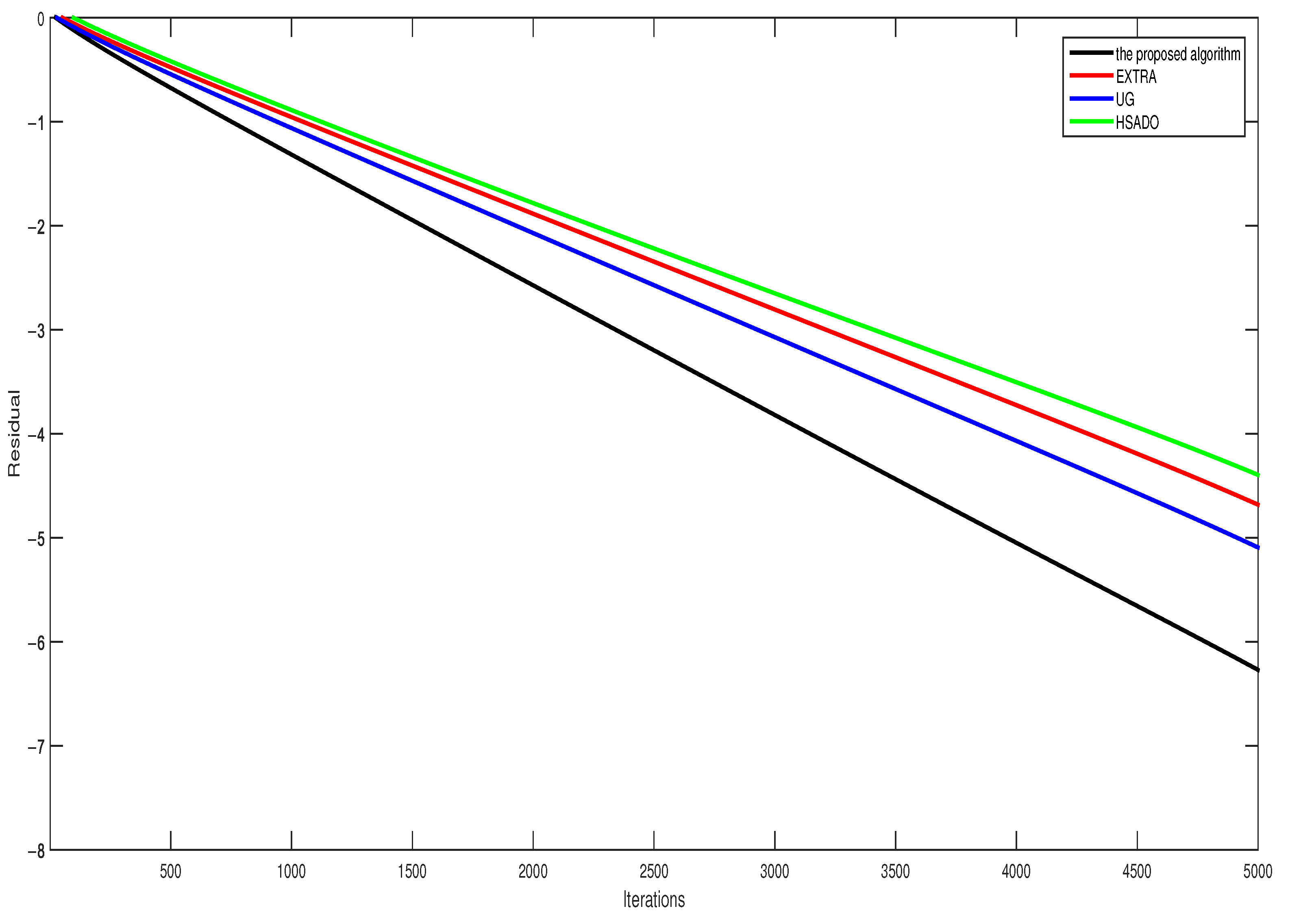
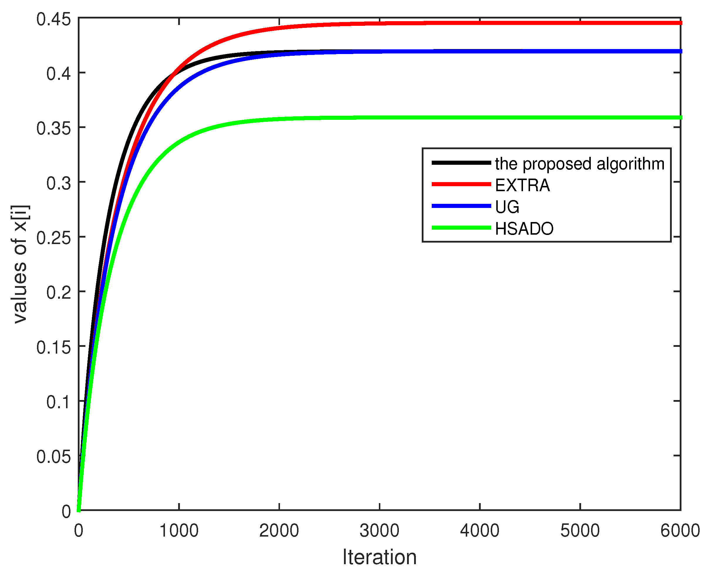
  • Figure 1 indicates that the proposed algorithm UGNH promotes the convergence rate compared to the related algorithms in the real dataset; thus, UGNH is effective and superior. From Figure 2, the sequences generated by UGNH, EXTRA, UG, and HSADO can converge to the optimal solutions as expected. Avoiding confusion of the figure, only one dimension of each decision variable is exhibited.
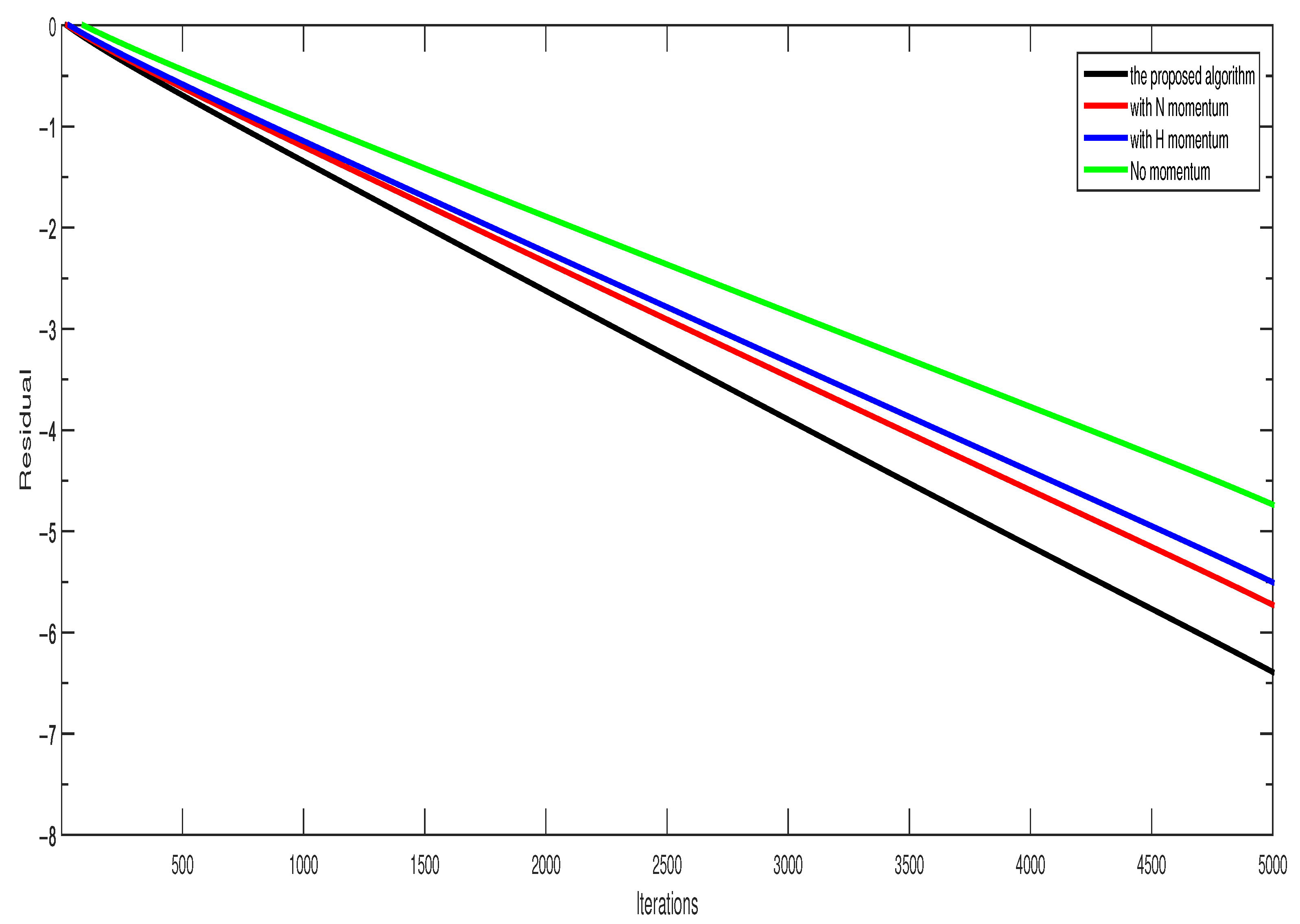
  • Figure 3 means that UGNH with the Nesterov momentum and the Heavy-ball momentum improved the convergence rate compared to the algorithm with only one or no momentum.
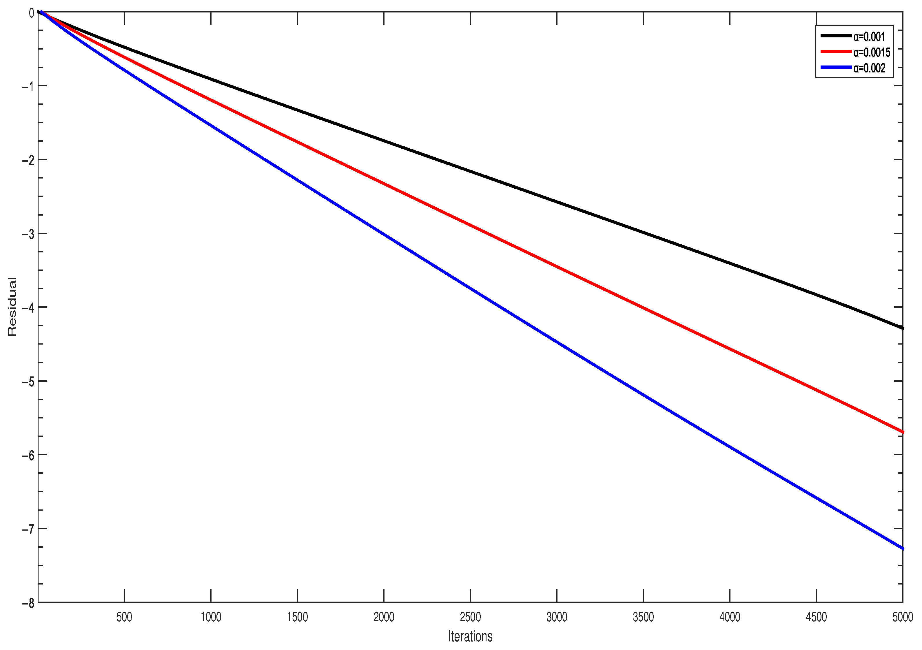
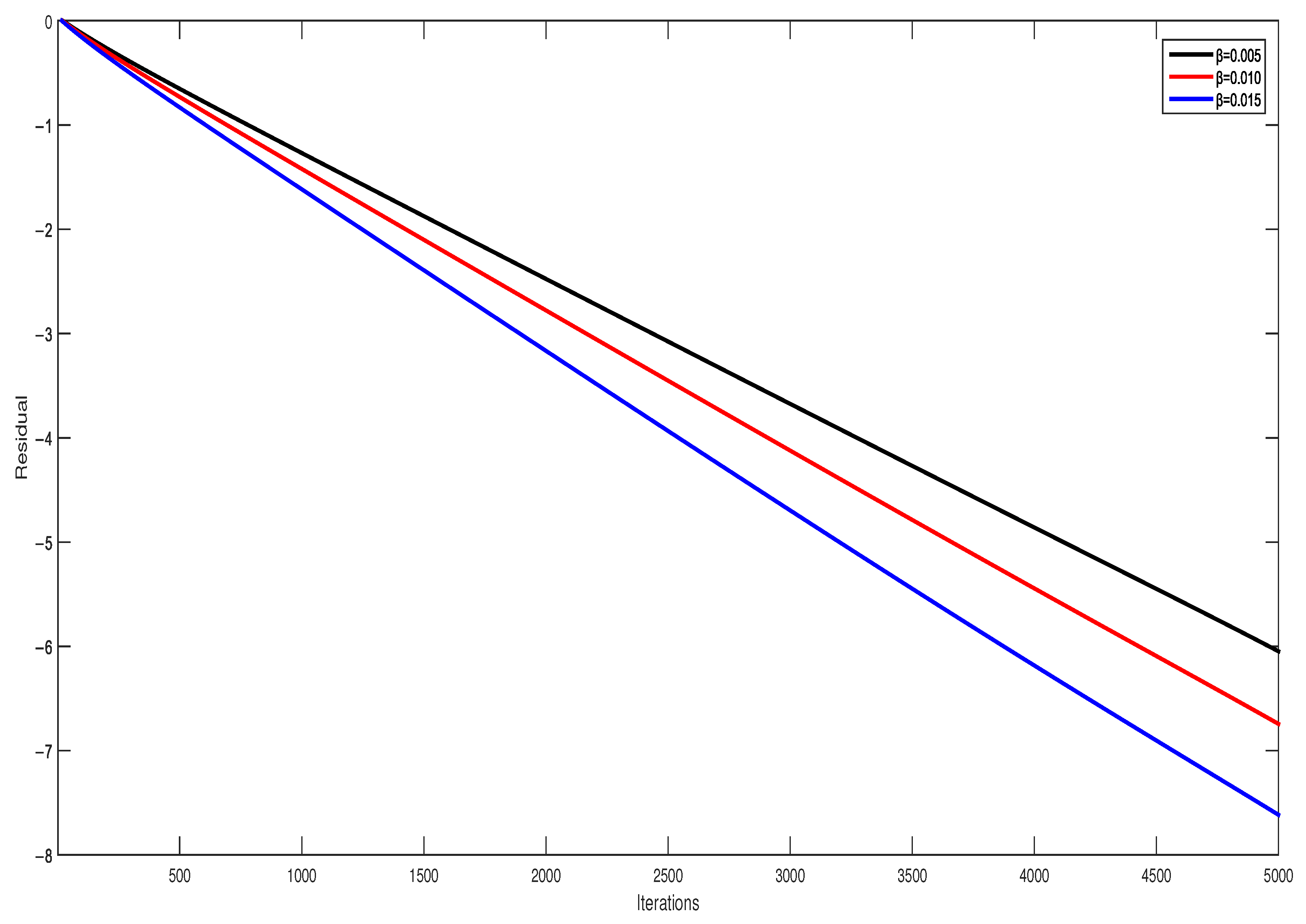
  • In Figure 4, we can conclude that step-size is usually chosen very small; the larger step-size leads to a faster convergence rate if it is chosen under the upper bound. For the coefficient, a similar result can be obtained in Figure 5. Comparing the two figures, it can be concluded that small changes in step-size are more influential than that of the coefficient.

6. Conclusions

In this study, a novel uncoordinated, time-varying, and nonidentical distributed optimization accelerated algorithm was proposed. It was mainly applied to handle the distributed optimization convex problem in an undirected network, where all agents are in an effort to optimize the average of all local objective functions collaboratively. When the largest step-size and the maximum coefficient do not exceed some estimated upper bounds, which have been provided in Theorem 1, the convergence rate of UGNH is linear under the condition that each local objective function is smooth and strongly convex. Besides, these parameters only depend on the topology of the network and the local objective function.
It is worth noting that to achieve a faster linear convergence rate, the Heavy-ball and Nesterov accelerated methods were simultaneously added into the algorithm, which provides a new way for accelerating convergence of other distributed optimization algorithms. Furthermore, the experiment results verified the effective and superior performance in a real dataset. However, UGNH is not suitable for all scenarios, and there are some more in-depth areas worth studying, such as the time-varying network architecture, random link failures, asynchronous communication between agents, directed networks, and so on. In all, these problems are worthy of further study and are our future research direction.

Author Contributions

Data curation, H.Z.; writing—original draft, Y.L.; supervision, X.G.; writing—review and editing, H.X. All authors have read and agreed to the published version of the manuscript.

Funding

This research was funded in part by the National Natural Science Foundation of China (41271292), in part by the Key Project of Chongqing Science and Technology Bureau (cstc2019jscx-gksbX0103), in part by the Fundamental Research Funds for the Central Universities under Project (SWU2009107), in part by the Chongqing Natural Science Foundation (cstc2020jcyj-msxmX0324), in part by the Key Project of Natural Science Research of Education Department in Anhui Province of China (KJ2019A0864), and in part by the Construction of Chengdu-Chongqing Economic Circle Science and Technology Innovation Project (KJCX2020007).

Institutional Review Board Statement

This paper does not studies involving human or animal.

Informed Consent Statement

This paper does not studies involving human or animal.

Data Availability Statement

The dataset can be fetched on the website http://archive.ics.uci.edu/ml, (accessed on 11 December 2021).

Conflicts of Interest

The authors declare no conflict of interest.

References

  1. Wang, H.; Liao, X.; Wang, Z.; Huang, T.; Chen, G. Distributed parameter estimation in unreliable sensor networks via broadcast gossip algorithms. Neural Netw. 2016, 73, 1–9. [Google Scholar] [CrossRef] [PubMed] [Green Version]
  2. Dougherty, S.; Guay, M. An extremum-seeking controller for distributed optimization over sensor networks. IEEE Trans. Autom. Control 2016, 62, 928–933. [Google Scholar] [CrossRef]
  3. Rahmani, A.M.; Ali, S.; Yousefpoor, M.S.; Yousefpoor, E.; Naqvi, R.A.; Siddique, K.; Hosseinzadeh, M. An area coverage scheme based on fuzzy logic and shuffled frog-leaping algorithm (sfla) in heterogeneous wireless sensor networks. Mathematics 2021, 9, 2251. [Google Scholar] [CrossRef]
  4. Ren, W. Consensus based formation control strategies for multi-vehicle systems. In Proceedings of the 2006 American Control Conference, Philadelphia, PA, USA, 14–16 June 2006; p. 6. [Google Scholar]
  5. Yan, B.; Shi, P.; Lim, C.C.; Wu, C.; Shi, Z. Optimally distributed formation control with obstacle avoidance for mixed-order multi-agent systems under switching topologies. IET Control Theory Appl. 2018, 12, 1853–1863. [Google Scholar] [CrossRef]
  6. Cevher, V.; Becker, S.; Schmidt, M. Convex optimization for big data: Scalable, randomized, and parallel algorithms for big data analytics. IEEE Signal Processing Mag. 2014, 31, 32–43. [Google Scholar] [CrossRef]
  7. Zhang, Z.; Wang, W.; Pan, G. A Distributed Quantum-Behaved Particle Swarm Optimization Using Opposition-Based Learning on Spark for Large-Scale Optimization Problem. Mathematics 2020, 8, 1860. [Google Scholar] [CrossRef]
  8. Li, K.; Liu, Q.; Yang, S.; Cao, J.; Lu, G. Cooperative optimization of dual multiagent system for optimal resource allocation. IEEE Trans. Syst. Man Cybern. Syst. 2018, 50, 4676–4687. [Google Scholar] [CrossRef]
  9. Jia, W.; Qin, S. Distributed Optimization Over Directed Graphs with Continuous-Time Algorithm. In Proceedings of the 2019 Chinese Control Conference (CCC), Guangzhou, China, 27–30 July 2019; pp. 1911–1916. [Google Scholar]
  10. Ahmed, E.M.; Rathinam, R.; Dayalan, S.; Fernandez, G.S.; Ali, Z.M.; Aleem, S.H.; Omar, A.I. A Comprehensive Analysis of Demand Response Pricing Strategies in a Smart Grid Environment Using Particle Swarm Optimization and the Strawberry Optimization Algorithm. Mathematics 2021, 9, 2338. [Google Scholar] [CrossRef]
  11. Zhang, Q.; Gong, Z.; Yang, Z.; Chen, Z. Distributed convex optimization for flocking of nonlinear multi-agent systems. Int. J. Control Autom. Syst. 2019, 17, 1177–1183. [Google Scholar] [CrossRef]
  12. Tang, X.; Li, M.; Wei, S.; Ding, B. Event-triggered Synchronous Distributed Model Predictive Control for Multi-agent Systems. Int. J. Control Autom. Syst. 2021, 19, 1273–1282. [Google Scholar] [CrossRef]
  13. Nedic, A.; Ozdaglar, A. Distributed subgradient methods for multi-agent optimization. IEEE Trans. Autom. Control 2009, 54, 48–61. [Google Scholar] [CrossRef]
  14. DeGroot, M.H. Reaching a consensus. J. Am. Stat. Assoc. 1974, 69, 118–121. [Google Scholar] [CrossRef]
  15. Ram, S.S.; Nedić, A.; Veeravalli, V.V. Distributed stochastic subgradient projection algorithms for convex optimization. J. Optim. Theory Appl. 2010, 147, 516–545. [Google Scholar]
  16. Nedic, A.; Ozdaglar, A.; Parrilo, P.A. Constrained consensus and optimization in multi-agent networks. IEEE Trans. Autom. Control 2010, 55, 922–938. [Google Scholar] [CrossRef]
  17. Duchi, J.C.; Agarwal, A.; Wainwright, M.J. Dual averaging for distributed optimization: Convergence analysis and network scaling. IEEE Trans. Autom. Control 2011, 57, 592–606. [Google Scholar] [CrossRef] [Green Version]
  18. Jakovetić, D.; Xavier, J.; Moura, J.M. Fast distributed gradient methods. IEEE Trans. Autom. Control 2014, 59, 1131–1146. [Google Scholar] [CrossRef] [Green Version]
  19. Shi, W.; Ling, Q.; Wu, G.; Yin, W. Extra: An exact first-order algorithm for decentralized consensus optimization. SIAM J. Optim. 2015, 25, 944–966. [Google Scholar] [CrossRef]
  20. Shi, W.; Ling, Q.; Wu, G.; Yin, W. A proximal gradient algorithm for decentralized composite optimization. IEEE Trans. Signal Processing 2015, 63, 6013–6023. [Google Scholar] [CrossRef]
  21. Xi, C.; Khan, U.A. DEXTRA: A fast algorithm for optimization over directed graphs. IEEE Trans. Autom. Control 2017, 62, 4980–4993. [Google Scholar] [CrossRef]
  22. Zeng, J.; Yin, W. Extrapush for convex smooth decentralized optimization over directed networks. arXiv 2015, arXiv:1511.02942. [Google Scholar]
  23. Yuan, K.; Ying, B.; Zhao, X.; Sayed, A.H. Exact diffusion for distributed optimization and learning-Part I: Algorithm development. IEEE Trans. Signal Processing 2018, 67, 708–723. [Google Scholar] [CrossRef] [Green Version]
  24. Yuan, K.; Ying, B.; Zhao, X.; Sayed, A.H. Exact diffusion for distributed optimization and learning-Part II: Convergence analysis. IEEE Trans. Signal Processing 2018, 67, 724–739. [Google Scholar] [CrossRef] [Green Version]
  25. Jakovetić, D.; Moura, J.M.; Xavier, J. Linear convergence rate of a class of distributed augmented lagrangian algorithms. IEEE Trans. Autom. Control 2014, 60, 922–936. [Google Scholar] [CrossRef] [Green Version]
  26. Qu, G.; Li, N. Harnessing smoothness to accelerate distributed optimization. IEEE Trans. Control Netw. Syst. 2017, 5, 1245–1260. [Google Scholar] [CrossRef] [Green Version]
  27. Nedic, A.; Olshevsky, A.; Shi, W. Achieving geometric convergence for distributed optimization over time-varying graphs. SIAM J. Optim. 2017, 27, 2597–2633. [Google Scholar] [CrossRef]
  28. Jakovetic, D.; Krejic, N.; Malaspina, G. Linear Convergence Rate Analysis of a Class of Exact First-Order Distributed Methods for Time-Varying Directed Networks and Uncoordinated Step Sizes. arXiv 2007, arXiv:2007.08837 2020. [Google Scholar]
  29. Nedić, A.; Olshevsky, A.; Shi, W.; Uribe, C.A. Geometrically convergent distributed optimization with uncoordinated step-sizes. In Proceedings of the 2017 American Control Conference (ACC), Seattle, WA, USA, 24–26 May 2017; pp. 3950–3955. [Google Scholar]
  30. Lu, Q.; Li, H.; Xia, D. Geometrical convergence rate for distributed optimization with time-varying directed graphs and uncoordinated step-sizes. Inf. Sci. 2018, 422, 516–530. [Google Scholar] [CrossRef] [Green Version]
  31. Qu, G.; Li, N. Accelerated distributed Nesterov gradient descent. IEEE Trans. Autom. Control 2019, 65, 2566–2581. [Google Scholar] [CrossRef] [Green Version]
  32. Xin, R.; Khan, U.A. Distributed heavy-ball: A generalization and acceleration of first-order methods with gradient tracking. IEEE Trans. Autom. Control 2019, 65, 2627–2633. [Google Scholar] [CrossRef] [Green Version]
  33. Mokhtari, A.; Ribeiro, A. DSA: Decentralized double stochastic averaging gradient algorithm. J. Mach. Learn. Res. 2016, 17, 2165–2199. [Google Scholar]
  34. Nedić, A.; Ozdaglar, A. Subgradient methods for saddle-point problems. J. Optim. Theory Appl. 2009, 142, 205–228. [Google Scholar] [CrossRef]
  35. Jakovetić, D. A unification and generalization of exact distributed first-order methods. IEEE Trans. Signal Inf. Processing Over Netw. 2018, 5, 31–46. [Google Scholar] [CrossRef] [Green Version]
  36. Xu, J.; Zhu, S.; Soh, Y.C.; Xie, L. Augmented distributed gradient methods for multi-agent optimization under uncoordinated constant stepsizes. In Proceedings of the 2015 54th IEEE Conference on Decision and Control (CDC), Osaka, Japan, 15–18 December 2015; pp. 2055–2060. [Google Scholar]
  37. Li, H.; Zheng, Z.; Lü, Q.; Wang, Z.; Gao, L.; Wu, G.C.; Ji, L.; Wang, H. Primal-Dual Fixed Point Algorithms Based on Adapted Metric for Distributed Optimization. IEEE Trans. Neural Netw. Learn. Syst. 2021, 2021, 1–15. [Google Scholar] [CrossRef]
  38. Liu, P.; Li, H.; Dai, X.; Han, Q. Distributed primal-dual optimisation method with uncoordinated time-varying step-sizes. Int. J. Syst. Sci. 2018, 49, 1256–1272. [Google Scholar] [CrossRef]
  39. Nesterov, Y. Introductory Lectures on Convex Optimization: A Basic Course; Springer Science & Business Media: Berlin/Heidelberg, Germany, 2003; Volume 87. [Google Scholar]
  40. Rivet, A.; Souloumiac, A. Introduction to Optimization. Optimization Software, Publications Division; Citeseer: Washington, DC, USA, 1987. [Google Scholar]
  41. Xin, R.; Khan, U.A. A linear algorithm for optimization over directed graphs with geometric convergence. IEEE Control Syst. Lett. 2018, 2, 315–320. [Google Scholar] [CrossRef] [Green Version]
  42. Cheng, H.; Li, H.; Wang, Z. On the convergence of exact distributed generalisation and acceleration algorithm for convex optimisation. Int. J. Syst. Sci. 2020, 51, 1–17. [Google Scholar] [CrossRef]
  43. Lü, Q.; Liao, X.; Li, H.; Huang, T. A nesterov-like gradient tracking algorithm for distributed optimization over directed networks. IEEE Trans. Syst. Man Cybern. Syst. 2020, 51, 6258–6270. [Google Scholar] [CrossRef]
  44. Hestenes, M.R.; Stiefel, E. Methods of Conjugate Gradients for Solving Linear Systems; NBS: Washington, DC, USA, 1952; Volume 49. [Google Scholar]
  45. Dua, D.; Graff, C. UCI Machine Learning Repository. 2017. Available online: http://archive.ics.uci.edu/ml (accessed on 11 December 2021).
Figure 1. Performance comparisons between the proposed algorithm and related algorithms.
Mathematics 10 00357 g001
Figure 2. One dimension of variable between the proposed algorithm and related algorithms.
Mathematics 10 00357 g002
Figure 3. Performance comparisons between the proposed algorithm and the method without momentum terms.
Mathematics 10 00357 g003
Figure 4. Performance comparisons between different step-sizes.
Mathematics 10 00357 g004
Figure 5. Performance comparisons between different momentum coefficients.
Mathematics 10 00357 g005
Publisher’s Note: MDPI stays neutral with regard to jurisdictional claims in published maps and institutional affiliations.

