Article

Fixed-Time Synchronization of Neural Networks Based on Quantized Intermittent Control for Image Protection

1
Chongqing Key Laboratory of Nonlinear Circuits and Intelligent Information Processing, College of Electronic and Information Engineering, Southwest University, Chongqing 400715, China
2
Key Laboratory of Machine Perception and Children’s Intelligence Development, Chongqing University of Education, Chongqing 400067, China
*
Authors to whom correspondence should be addressed.
Mathematics 2021, 9(23), 3086; https://doi.org/10.3390/math9233086
Submission received: 10 November 2021 / Revised: 25 November 2021 / Accepted: 26 November 2021 / Published: 30 November 2021
(This article belongs to the Special Issue Modeling and Analysis of Complex Networks)

Abstract

:
This paper considers the fixed-time synchronization (FIXTS) of neural networks (NNs) by using quantized intermittent control (QIC). Based on QIC, a fixed-time controller is designed to ensure that the NNs achieve synchronization in finite time. With this controller, the settling time can be estimated regardless of initial conditions. After ensuring that the system has stabilized through this strategy, it is suitable for image protection given the behavior of the system. Meanwhile, the encryption effect of the image depends on the encryption algorithm, and the quality of the decrypted image depends on the synchronization error of NNs. The numerical results show that the designed controller is effective and validate the practical application of FIXTS of NNs in image protection.

1. Introduction

With the rapid development of the internet and the increased exchange of information in the network [1], information security becomes particularly important [2,3]. When data is transmitted, it can be subject to network attacks, which can lead to data leakage. Therefore, for reasons of data security, encryption algorithms are widely used in secure communications, especially in digital image processing [4,5,6,7]. In [4], a new technique is proposed to create chaos-based encryption schemes with larger parameter spaces using chaotic maps with adaptive symmetry. Furthermore, chaotic encryption algorithms have received a great deal of attention due to their unpredictability and extreme sensitivity of the initial conditions [6,8,9]. However, not all chaotic encryption algorithms guarantee the possibility of lossless decryption. Therefore, we choose a chaotic encryption algorithm the synchronization of NNs [7,10], which can guarantee the decryption of the image after the error system is synchronized. In [7], a chaotic cryptosystem using a synchronous chaotic system as a key generator is proposed. Thus, the security of medical image transmission and storage can be improved. Up to now, there has been considerable research into the synchronization of NNs. Among them, finite-time synchronization (FTS) has been extensively studied because of its ability to converge in a relatively short period of time [11,12,13,14]. In [12], the main study is the FTS of coupled neural networks when the controller is discontinuous; in [14], the main study is FTS of neural networks with time delays.
However, finite-time synchronization also has its drawbacks in that the estimate of the FTS establishment time depends on changes in the initial conditions of the system [15]. However, the initial values of the system are more difficult to obtain [16]. For example, in secure communication, how should one decrypt an image after applying chaotic encryption when the initial values of the system are not available? Reference [17] proposes a special kind of FTS, namely FIXTS, that can solve this problem. The estimated time establishment for FIXTS does not depend on the initial value of the system. Thus, it can be used to decrypt chaotic encrypted images that lack a systematic initial value. Therefore, it is important to study chaotic encryption algorithms based on fixed-time synchronization of neural networks in image protection.
Fixed-time synchronization of neural networks by designing a new controller. In recent decades, researchers have proposed many different control methods to stabilise various systems, such as adaptive control [18], pinning control [19,20], intermittent control [21] and sliding mode control [22,23]. As intermittent control has a discontinuous working time, control costs can be reduced. Therefore, it is more beneficial for applications in the engineering field. In addition, since the communication channel capacity is also limited [24], we have considered signal quantization in the design of the controller [25,26]. Thus, this paper investigates fixed-time synchronization of neural networks based on quantized interval control, after which the synchronized sequences are used for image encryption and decryption.
Motivated by the aforementioned concerns, this paper proposes a method of quantized intermittent control to ensure that the neural networks achieves FIXTS and applies the synchronization sequence to image protection. The contributions and innovations of this paper can be summarised as follows.
(1) Considering the limited channel capacity and control costs, a combination of intermittent control and quantization strategies is therefore used. Neural network synchronization is achieved by this method.
(2) A fixed time controller was designed through which the fixed time synchronization of the neural network was achieved. In contrast to FTS, the estimated time for FIXTS is established independent of the initial conditions.
(3) Applying chaotic neural networks and fixed-time synchronization techniques to the encryption and decryption of images. The application of this chaotic neural network enables the image encryption system to resist stronger security attacks and has greater robustness.
The chapter arrangement of this paper is as follows: in Section 2, the system model is presented, with some useful definitions and assumptions. In in Section 3, the fixed-time synchronization of neural networks and its strict derivation are studied. In in Section 4, the theoretical results are verified by example and simulation results. Furthermore, apply fixed-time synchronization to image protection. In in Section 5, the conclusion is given.

2. Preliminaries and System Description

Consider the following NNs for i = 1 , 2 , , n :
m ˙ i ( ς ) = c i m i ( ς ) + j = 1 n a i j f j ( m i ( ς ) ) ,
where ς indicates the time scale, m ( ς ) = ( m 1 ( ς ) , m 2 ( ς ) , , m n ( ς ) ) T R n is the state vector of the neural networks, f ( m ( ς ) ) = ( f 1 ( m 1 ( ς ) ) , f 2 ( m 2 ( ς ) ) , , f n ( m n ( ς ) ) T is vector-valued activation function. C = d i a g ( c 1 , c 2 , , c n ) > 0 is the self-feedback connection weight matrix, A = ( a i j ) n × n is a synaptic connection weight matrix.
In order to facilitate understanding, we take the system (1) as the drive system, the response system is shown in the following equation:
χ ˙ i ( ς ) = c i χ i ( ς ) + j = 1 n a i j f j ( χ i ( ς ) ) + u i ( ς ) ,
where i = 1 , 2 , n , χ ( ς ) = ( χ 1 ( ς ) , χ 2 ( ς ) , , χ n ( ς ) ) T R n is the state vector of the neural networks, f ( χ ( ς ) ) = ( f 1 ( χ 1 ( ς ) ) , f 2 ( χ 2 ( ς ) ) , , f n ( χ n ( ς ) ) T is vector-valued activation function. u i ( ς ) is a controller; C = d i a g ( c 1 , c 2 , , c n ) > 0 is the self-feedback connection weight matrix, A = ( a i j ) n × n is a synaptic connection weight matrix.
Definition 1
([27]). If there exists a constant T > 0 such that the following inequality holds:
lim ς T m i ( ς ) χ i ( ς ) = 0 .
for any i = 1 , 2 , , n , if ς T , then the drive system (1) and the response system (2) are said to be FIXTS.
Assumption A1
([24]). f : R n R n are nonlinear functions satisfying the Lipstchiz condition and there exist constant L 0 , such that:
f ( χ i ( ς ) ) f ( m i ( ς ) ) L χ i ( ς ) m i ( ς ) ,
where i = 1 , 2 , , n and χ i ( ς ) , m i ( ς ) R .
Lemma 1
([28]). If V ( ς ) is a non-negative function and satisfies the following conditions:
V ˙ ( ς ) a V p ( ς ) b V q ( ς ) , ς [ k T , k T + σ T ) , V ˙ ( ς ) 0 , ς [ k T + σ T , ( k + 1 ) T ) ,
where T > 0 , 0 < σ < 1 , k = 0 , 1 , 2 , , a > 0 , b > 0 , 0 < p < 1 , q > 1 . Then V ( ς ) 0 , if
ς T m a x = 1 a σ ( 1 p ) + 1 b σ ( q 1 ) .
Lemma 2
([29]). If 0 < p 1 , q > 1 and η 1 , η 2 , , η n 0 , then
i = 1 n η i p ( i = 1 n η i ) p , i = 1 n η i q n 1 q ( i = 1 n η i ) q .
Lemma 3
([30]). If there exists a positive constant γ and a positive definite symmetric matrix Λ, then for any matrices P and Q the following inequality holds:
P T Q + Q T P γ P T Λ P + γ 1 Q T Λ 1 Q .

3. Main Results

In this section, we will study the fixed-time synchronization of neural networks via QIC. Define ϑ i ( ς ) = χ i ( ς ) m i ( ς ) as the error system, thus, the error dynamics system can be expressed as:
ϑ ˙ i ( ς ) = c i ϑ i ( ς ) + j = 1 n a i j g j ( ϑ i ( ς ) ) + u i ( ς ) ,
where g j ( ϑ i ( ς ) ) = f j ( χ i ( ς ) ) f j ( m i ( ς ) ) .
In order to achieve FIXTS, the quantized intermittent controller is designed as follows:
u i ( ς ) = r 1 q ( ϑ i ( ς ) ) r 2 s g n ( q ( ψ i ( ς ) ) ) ( | ϑ i ( ς ) | α + | ϑ i ( ς ) | β ) , ς [ k T , k T + σ T ) , u i ( ς ) = r 1 q ( ϑ i ( ς ) ) , ς [ k T + σ T , ( k + 1 ) T ) ,
where 0 < α < 1 , β > 1 , r 1 > 0 , r 2 > 0 , 0 < σ < 1 .
Furthermore, ω = ± ω i : ω i = ρ i ω 0 , 0 < ρ < 1 , i = 0 , ± 1 , ± 2 , 0 with a sufficiently large constant ω 0 > 0 . For τ R , q ( τ ) is constructed as follows:
q ( τ ) = ω i , i f 1 1 + δ ω i < τ 1 1 δ ω i , 0 , i f τ = 0 , q ( τ ) , i f τ < 0 ,
where δ = 1 ρ 1 + ρ . According to the analysis in [24], if Δ [ δ , δ ] exists in Equation (10), then q ( τ ) = ( 1 + Δ ) τ , τ R . Furthermore, at the same time if Λ ( ς ) = d i a g ( Λ 1 ( ς ) , Λ n ( ς ) ) , and Λ i ( ς ) [ δ , δ ] , i = 1 , 2 n , then:
q ( ϑ i ( ς ) ) = ( I n + Λ ( ς ) ) ϑ i ( ς ) .
Theorem 1.
If the following inequalities hold, the error system (9) will be stable in a fixed time T m a x .
C + λ 1 A A T + λ 1 1 L + r 1 ( 1 + δ ) + 2 r 2 < 0 , C + λ 1 A A T + λ 1 1 L + r 1 ( 1 + δ ) < 0 ,
where λ 1 and L are positive constants, and r 1 > 0 , r 2 > 0 , 0 < σ < 1 , 0 < δ < 1 .
Consequently, the response system (2) is fixed-timely synchronized onto drive system (1) under the controller (10). The fixed time can be estimated by:
T m a x = 1 2 r 2 σ 1 α 2 + 1 2 r 2 σ β 1 2 .
where r 2 is the control gain parameter and σ is the intermittent control parameter.
Proof. 
Based on the Lyapunov method, if a perturbation is given to the system, when the perturbation disappears, the stored energy of the system will gradually decay until it tends to the equilibrium state, and the energy of the system tends to a minimal value. Furthermore, the Lyapunov function is designed as follows:
V ( ς ) = ϑ i ( ς ) T ϑ i ( ς ) .
The Lyapunov function is derived and take the derivative of V ( ς ) at different time periods of the quantized intermittent controller (10), as follows:
When ς [ k T , k T + σ T )
ϑ ˙ i ( ς ) = C ψ i ( ς ) + A g ( ϑ i ( ς ) ) r 1 q ( ϑ i ( ς ) ) r 2 s g n ( q ( ϑ i ( ς ) ) ) | ϑ i ( ς ) | α + | ϑ i ( ς ) | β .
Then,
V ˙ ( ς ) = ϑ i ( ς ) T 2 ϑ ˙ i ( ς ) = ϑ i ( ς ) T 2 ( C ϑ i ( ς ) + A g ( ϑ i ( ς ) ) r 1 q ( ϑ i ( ς ) ) r 2 s g n ( q ( ϑ i ( ς ) ) ) ( | ϑ i ( ς ) | α + | ϑ i ( ς ) | β ) ) = ϑ i ( ς ) T 2 C ψ i ( ς ) + 2 ϑ i ( ς ) T A g ( ϑ i ( ς ) ) ϑ i ( ς ) T 2 r 1 q ( ϑ i ( ς ) ) 2 ϑ i ( ς ) T r 2 s g n ( q ( ϑ i ( ς ) ) ) | ϑ i ( ς ) | α 2 ϑ i ( ς ) T r 2 s g n ( q ( ϑ i ( ς ) ) ) | ϑ i ( ς ) | β .
By using Assumption 1 and Lemma 3, where λ 1 is a positive constant and the following inequality holds:
2 ϑ i ( ς ) T A g ( ψ i ( ς ) ) λ 1 ϑ i ( ς ) T A A T ϑ i ( ς ) + λ 1 1 g ( ϑ i ( ς ) ) T g ( ϑ i ( ς ) ) λ 1 ϑ i ( ς ) T A A T ϑ i ( ς ) + λ 1 1 L ϑ i ( ς ) T ϑ i ( ς ) ,
Using Equation (12), then:
ϑ i ( ς ) T q ( ϑ i ( ς ) ) = ϑ i ( ς ) T ( I + Δ ( ς ) ) ϑ i ( ς ) ϑ i ( ς ) T ( 1 + δ ) ϑ i ( ς ) ,
Accordng to (12) and δ < 1 , if ϑ i ( ς ) > 0 ( o r < 0 ) , then q ( ϑ i ( ς ) ) > 0 ( o r < 0 ) . Hence,
s g n ( q ( ϑ i ( ς ) ) ) = s g n ( ϑ i ( ς ) ) ,
Then,
ϑ i ( ς ) T r 2 s g n ( q ( ϑ i ( ς ) ) ) | ϑ i ( ς ) | α = ϑ i ( ς ) T r 2 s g n ( ϑ i ( ς ) ) | ϑ i ( ς ) | α r 2 | ϑ i ( ς ) T ϑ i ( ς ) | α + 1 2 , ϑ i ( ς ) T r 2 s g n ( q ( ϑ i ( ς ) ) ) | ϑ i ( ς ) | β = ϑ i ( t ) T r 2 s g n ( ϑ i ( ς ) ) | ϑ i ( ς ) | β r 2 | ϑ i ( ς ) T ϑ i ( ς ) | β + 1 2 .
Therefore,
V ˙ ( ς ) ϑ i ( ς ) T 2 | | C | | ϑ i ( ς ) + λ 1 ϑ i ( ς ) T A A T ϑ i ( ς ) + λ 1 1 L ϑ i ( ς ) T ϑ i ( ς ) + ϑ i ( ς ) T 2 r 1 ( 1 + δ ) ϑ i ( ς ) 2 r 2 | ϑ i ( ς ) T ϑ i ( ς ) | α + 1 2 2 r 2 | ϑ i ( ς ) T ϑ i ( ς ) | β + 1 2 ϑ i ( ς ) T 2 C + λ 1 A A T + λ 1 1 L + r 1 ( 1 + δ ) ϑ i ( ς ) 2 r 2 | ϑ i ( ς ) T ϑ i ( ς ) | α + 1 2 2 r 2 | ϑ i ( ς ) T ϑ i ( ς ) | β + 1 2 .
By inequalities (13), then
V ˙ ( ς ) 2 r 2 | ϑ i ( ς ) T ϑ i ( ς ) | α + 1 2 2 r 2 | ϑ i ( ς ) T ϑ i ( ς ) | β + 1 2 = 2 r 2 V α + 1 2 2 r 2 V β + 1 2 .
Similarly, when ς [ k T + σ T , ( k + 1 ) T )
ϑ ˙ ( ς ) = C ϑ i ( ς ) + A g ( ϑ i ( ς ) ) r 1 q ( ϑ i ( ς ) )
then
V ˙ ( ς ) = ϑ i ( ς ) T 2 ϑ ˙ i ( ς ) = ϑ i ( ς ) T 2 C ϑ i ( ς ) + A g ( ϑ i ( ς ) ) r 1 q ( ϑ i ( ς ) ) = ϑ i ( ς ) T 2 C ϑ i ( ς ) + 2 ϑ i ( ς ) T A g ( ϑ i ( ς ) ) ϑ i ( ς ) T 2 r 1 q ( ϑ i ( ς ) ) ϑ i ( ς ) T 2 C ϑ i ( ς ) + λ 1 ϑ i ( ς ) T A A T ϑ i ( ς ) + λ 1 1 L ϑ i ( ς ) T ϑ i ( ς ) + ϑ i ( ς ) T 2 r 1 ( 1 + δ ) ϑ i ( ς ) ϑ i ( ς ) T 2 C + λ 1 A A T + λ 1 1 L + r 1 ( 1 + δ ) ϑ i ( ς ) .
By inequalities (13), then
V ˙ ( ς ) 0 .
For ς R n , we have:
V ˙ ( ς ) 2 r 2 V α + 1 2 2 r 2 V β + 1 2 , ς [ k T , k T + σ T ) , V ˙ ( ς ) 0 , ς [ k T + σ T , ( k + 1 ) T ) ,
where r 2 is the control gain parameter and σ is the intermittent control parameter. Under the Lemma 1, let a = 2 r 2 , b = 2 r 2 , p = α + 1 2 , q = β + 1 2 , then we have T m a x = 1 2 r 2 σ 1 α 2 + 1 2 r 2 σ β 1 2 . It follows that, V ( ς ) 0 , if ς > T m a x . Moreover, the system error ϑ i ( ς ) will converge to zero within T m a x . Consequently, under the controller (10), the response system (2) is fixed-timely synchronized onto the drive system (1). This completes the proof.    □
Remark 1.
In inequalities (18), if the Intermittent control parameter σ = 0 or σ = 1 , the discrete time controller (10) will become a continuous time controller. To date, researchers have made in-depth analyses of continuous-time systems, and relevant details can be found in [31,32,33]. Similarly, the drive system (1) and the response system (2) can be synchronized.
Remark 2.
When the intermittent control parameter σ = 0 , the controller is expressed as follows
u i ( ς ) = r 1 q ( ϑ i ( ς ) ) .
When the intermittent control parameter σ = 1 , the controller of a system is expressed as follows
u i ( ς ) = r 1 q ( ϑ i ( ς ) ) r 2 s g n ( q ( ϑ i ( ς ) ) ) .
Remark 3.
From Equation (14), we can see that the establishment of the estimated time for FIXTS is closely related to r 2 . When the parameter α , β , σ are constants, T m a x = 1 2 r 2 σ 1 α 2 + 1 2 r 2 σ β 1 2 will become a strictly decreasing function with respect to the parameter r 2 . As a result, we can control the estimation time by adjusting the value of r 2 .

4. Numerical Simulation: Synchronized and Applied to Image Encryption

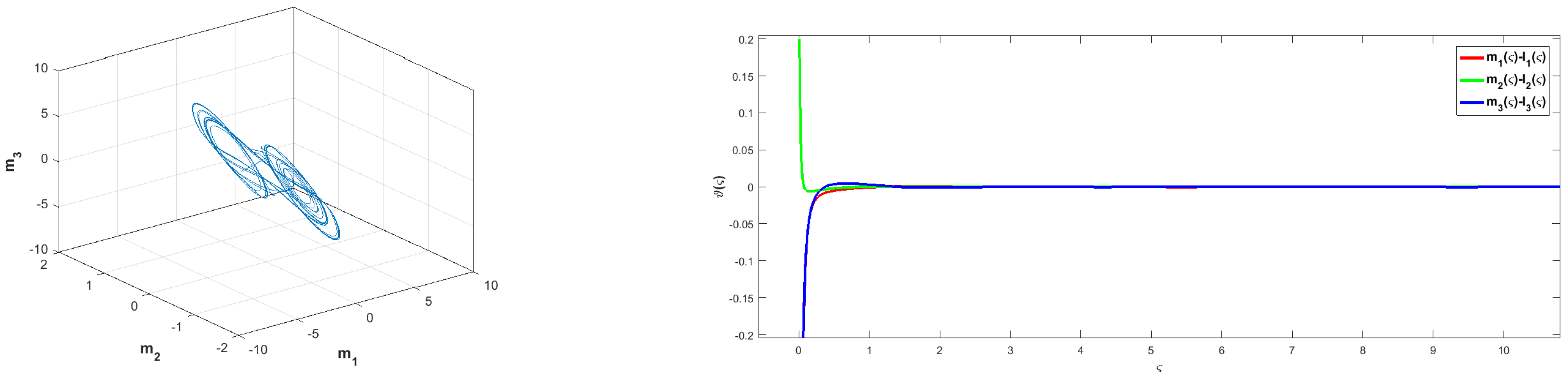
4.1. FIXTS of Neural Networks via Quantized Intermittent Control

In this section, we will verify the correctness of the controller (10) design by means of a simulation example, thus proving the correctness of Theorem 1.
The Chua’s circuit equation consider neural networks described by the following equation to illustrate Theorem 1 [34]:
m ˙ ( ς ) = C m ( ς ) + A f ( m ( ς ) ) ,
where m ( ς ) = ( m 1 ( ς ) , m 2 ( ς ) , m 3 ( ς ) ) T , f ( m ( ς ) ) = 0.5 ( | m 1 ( ς ) + 1 | | m 1 ( ς ) 1 | , 0 , 0 ) T , A = d i a g ( 54 / 7 , 0 , 0 ) ,
C = 19 7 9 0 1 1 1 0 14.28 0 .
When the initial state of m ( 0 ) = ( 0.65 , 0.2 , 0.8 ) T , the chaotic attractor can be observed according to Figure 1a.
Consider the error system as follows:
ϑ ˙ ( ς ) = C ϑ ( ς ) + A g ( ϑ ( ς ) ) + u ( ς ) ,
where u ( ς ) is a controller, the controller as follows:
u ( ς ) = r 1 q ( ϑ ( ς ) ) r 2 s g n ( q ( ϑ ( ς ) ) ) ( | ϑ ( ς ) | α + | ϑ ( ς ) | β ) , ς [ k T , k T + σ T ) , u ( ς ) = r 1 q ( ϑ ( ς ) ) , ς [ k T + σ T , ( k + 1 ) T ) ,
where 0 < σ < 1 is an intermittent adjustment parameter and 0 < δ = 1 ρ 1 + ρ < 1 is a parameter related to quantification, we choose σ = 0.4 , ρ = 0.6 , then δ = 1 ρ 1 + ρ = 0.25 . According to the inequalities (13) and L = 1 , λ 1 = 1 , we can obtain the gain parameters of the controller r 1 > 47.377 and 0 < r 2 < 0.375 r 1 17.7664 . We choose r 1 = 60 and 0 < r 2 < 4.7336 , then choose r 2 = 4 . Furthermore, α > 0 , β > 1 , then choose α = 0.5 , β = 1.5 . Therefore, under the controller (23), the error system is stabilized, which is shown in Figure 1b. Furthermore, by (14), one can estimate the settling time by T m a x = 1.6667  (s). From Figure 1b, one can get that the synchronization error approaches to zero before 1.6667  (s). This suggests that Theorem 1 is correct.

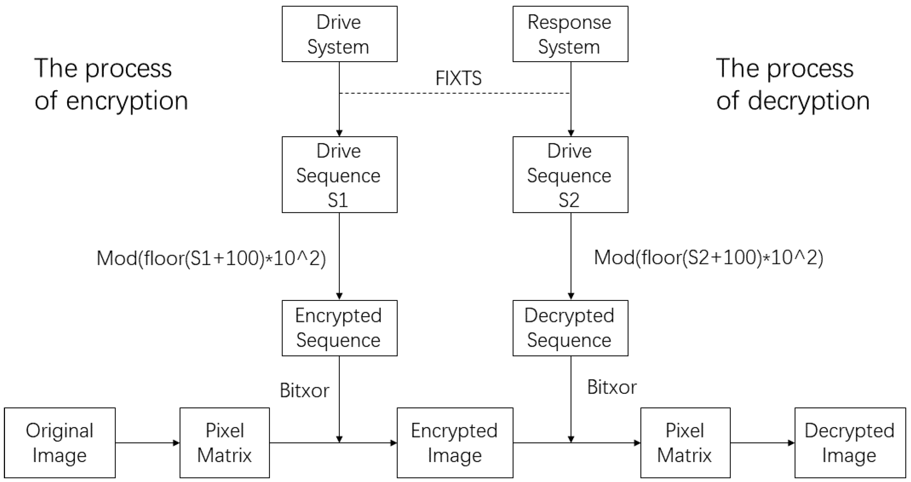
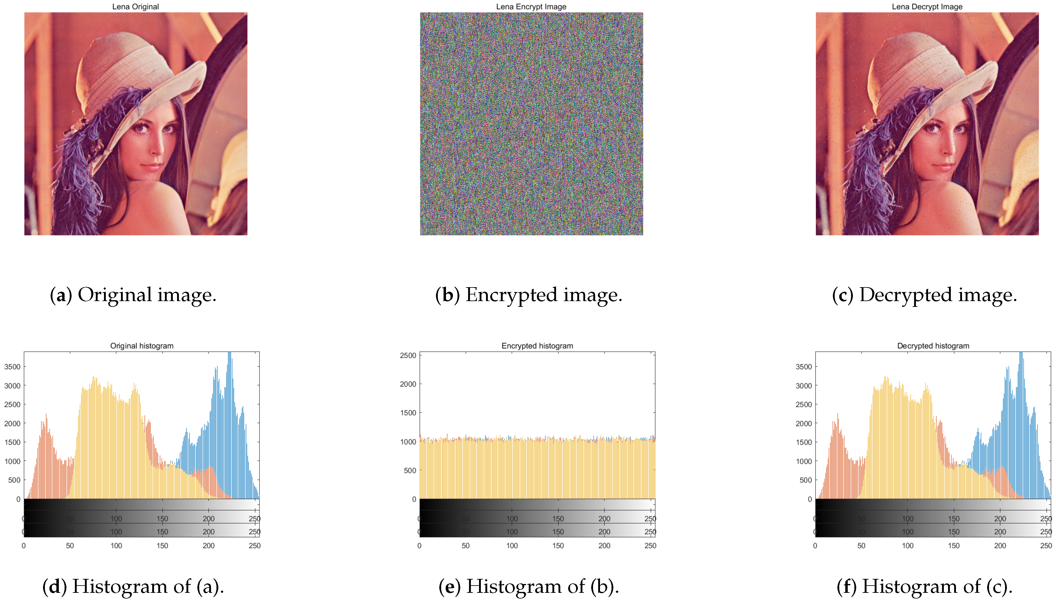
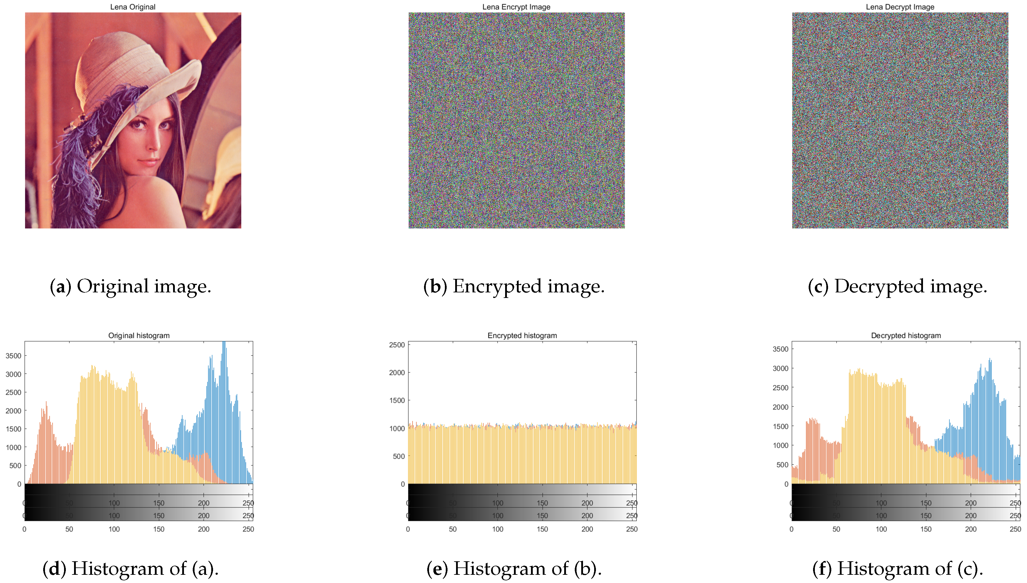
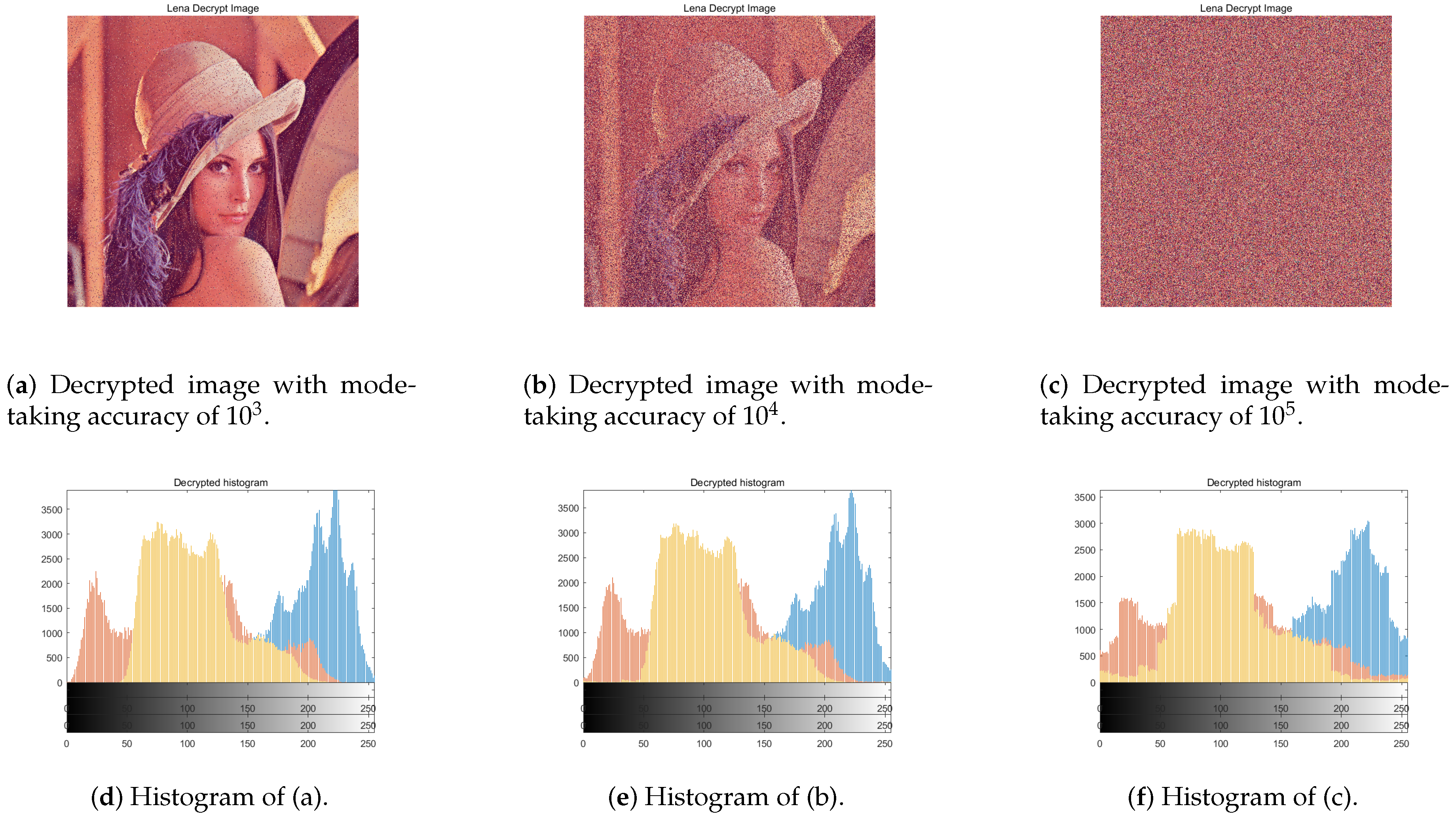
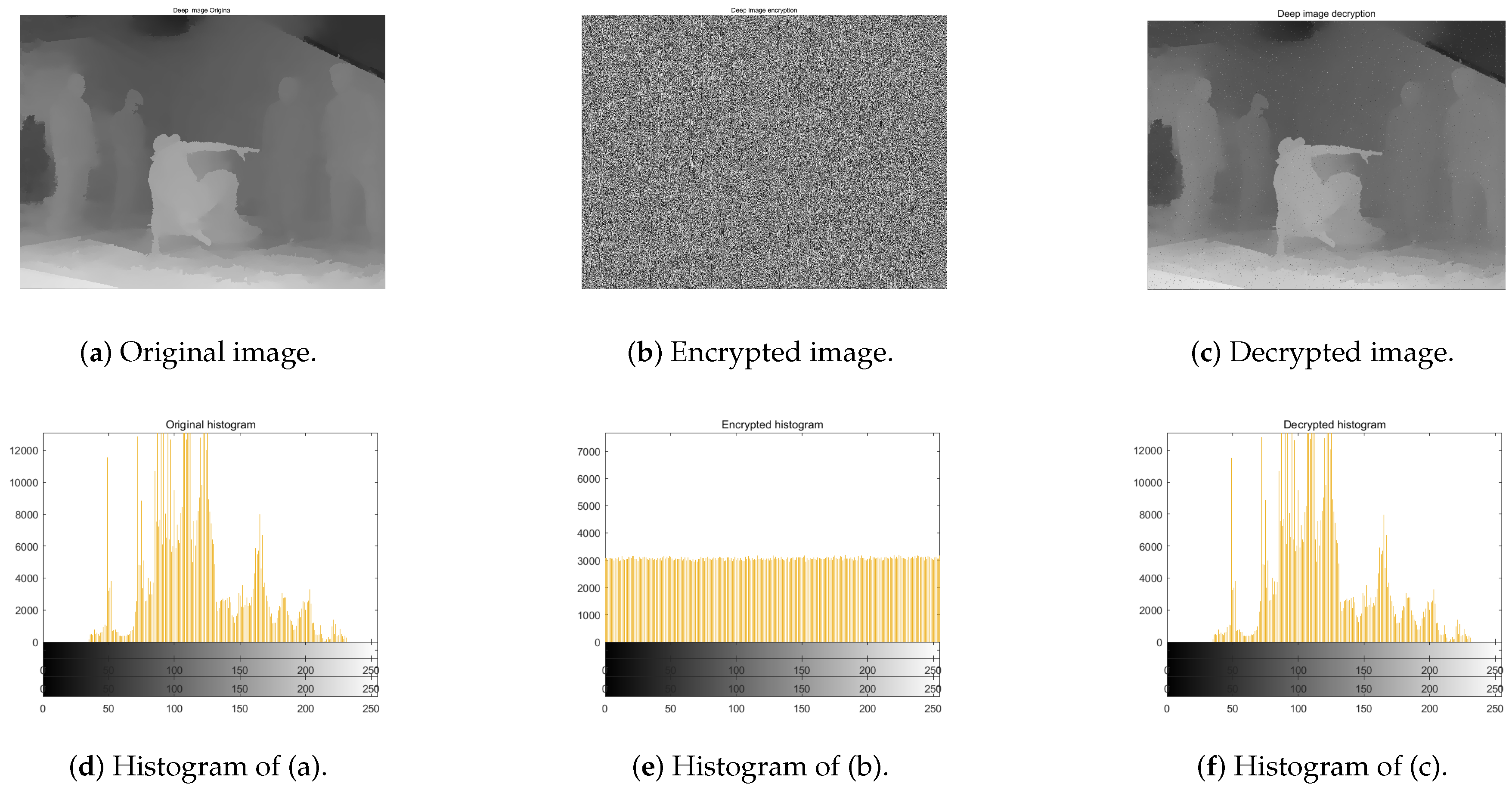
4.2. Application of FIXTS to Image Protection

In this section, we apply Theorem 1 to image protection. When the NNs achieves FIXTS, the drive system sequence is applied to the image encryption and the response system sequence is used as the decryption sequence for the encrypted image (see Figure 2).
I . Chaotic Encryption and Decryption Mechanism: Choose a picture P (lena.tiff) with a size M × N × 3 , then the image encryption described as follows.
( 1 ) . Assume that the pixel size of image P is M × N and that the pixel values are all integers from 0 to 255. Then, the pixel values of image P are read through the three channels R, G and B. Therefore, three grey scale images P R ( i , j ) , P G ( i , j ) and P B ( i , j ) can be obtained.
( 2 ) . Obtain the sequence S 1 of the drive system after achieving FIXTS and integerise the sequence S 1 as follows.
X 1 = m o d ( f l o o r ( S 1 + 100 ) * 10 2 , 10 * m a x ( M , N ) ) + 2 , S = m o d ( f l o o r ( ( S 1 + 1000 ) * 10 2 ) , 256 ) .
The resulting X 1 is the pseudo-random sequence and S is the diffusion pseudo-random sequence. Then, the dislocation pseudorandom sequences X 1 p and X 1 n are generated by X 1 , and the forward diffusion pseudorandom sequence S 1 p and the inverse diffusion pseudorandom sequence S 1 n are generated by S.
( 3 ) . Disorder the grey-scale images P R ( i , j ) , P G ( i , j ) , P B ( i , j ) with the Arnold matrix, the disorder steps are as follows.
m o d ( X 1 n ( k ) + X 1 p * k , M * N ) + 1 , k = 1 , 2 , , M * N .
As a result, the images M R ( i , j ) , M G ( i , j ) and M B ( i , j ) can be obtained after the dislocation.
( 4 ) . The forward diffusion and reverse diffusion of the scrambled images M R ( i , j ) , M G ( i , j ) and M B ( i , j ) are performed based on the heteroskedastic operation, so that the encrypted images E R ( i , j ) , E G ( i , j ) and E B ( i , j ) can be obtained. The specific encryption algorithm is shown in Algorithm 1 (taking image M B ( i , j ) as an example):
Algorithm 1 Diffusion processing(eg:image M B ( i , j ) )
Input:
MB(i,j),  M,  N,   S 1 p ,   S 1 n .
Output:
EB(i,j).
1:
B(i) = MB(:);
2:
B 0 = 0, B 1 = zeros(1, M * N);
3:
B 1 (1) = bitxor(bitxor( B 0 , S 1 p ),B(1));
4:
for i = 2 : M * N  do
5:
    B 1 ( i ) = bitxor(bitxor( B 1 ( i 1 ) , S 1 p ( i ) ), B 1 ( i ) );
6:
end for
7:
B 2 = zeros(1, M * N);
8:
B 2 ( i ) = bitxor(bitxor( B 0 , S 1 n ( M * N ) ), B 1 ( M * N ) );
9:
for i = M * N 1 : 1 :1 do
10:
    B 2 ( i ) = bitxor(bitxor( B 2 ( i + 1 ) , S 1 n ( i ) ), B 1 ( i ) );
11:
end for
12:
EB(i,j) = reshape( B 2 ,M,N);
13:
return EB(i,j);
( 5 ) . The decryption process, by selecting the response system sequence S and carrying out the reverse process of steps (1)–(4), results in the decrypted images DR, DG and DB, and finally the three grayscale images are synthesized, which is the decrypted image P (lena.tiff).
I I . Experimental Results: In this section, specific simulation examples are analysed in order to determine the effectiveness of FIXTS of NNs applied to image protection. In Example 1 the image l e n a is analysed for encryption and decryption and other related image analysis. In Example 2 the encryption and decryption algorithm is performed on the depth image. In Example 3 the corresponding comparison with articles of the similar type is given. Example 4 gives the performance analysis of the execution of encryption and decryption algorithms for images.
Example 1.
Image encryption and decryption.
A image (lena.tiff) of size 256 × 256 was selected for simulation verification. From Figure 3a–c it can be seen that the lena has been encrypted by the drive system sequence and is able to recover the lena by decrypting it in response to the system sequence. From the histogram of the information distribution in Figure 3d–f, it can be observed that the image information has been completely hidden and then recovered again afterwards.
Table 1 shows the correlation of adjacent pixels of the three images acquired by the lena plot through the R, G and B channels. By analysing the correlation of adjacent pixels in the horizontal, vertical and diagonal directions of the image. From the table, it is clear that the correlation of adjacent pixel points after lena has been encrypted almost converges to zero, thus demonstrating the effectiveness of applying FIXTS of NNs to image protection. Comparing the correlation between the original image and the decrypted image, we can see that the correlation between the adjacent pixels of the decrypted image is close to that of the original image, thus proving that our decryption algorithm works well.
Figure 4a–f shows what happens when the neural network does not implement fixed time synchronization. From Figure 4a–c it is known that the image is not recoverable, verifying that when the system is not synchronized, the response system sequence cannot be obtained and therefore the decrypted image cannot be decrypted. Thus, the performance of the image encryption algorithm proposed in this paper is demonstrated.
Figure 5 represents the lena diagram as a decrypted image based on fixed time synchronization with different mould taking accuracy. Figure 5a indicates the synchronization of the error system with mode-taking accuracy of 10 3 , Figure 5b indicates the synchronization of the error system with mode-taking accuracy of 10 4 and Figure 5c indicates the synchronization of the error system with mode-taking accuracy of 10 5 . The effect of the synchronization of the error system with mode-taking accuracy on the quality of the image decryption can be seen in Figure 5a–c. Figure 5 illustrates the sensitivity of the decryption sequences, when the synchronization error system has different mode-taking accuracy, the resulting decryption sequences are different, and thus the quality of the decrypted images is also different.
Example 2.
Encryption and decryption of deep images.
Applying the encryption and decryption algorithm of the image to the depth image, it can be seen in Figure 6a–c that the depth image is encrypted and then restored to the depth image. It can be observed from Figure 6e that the depth image information has been completely hidden, and Figure 6f has been re-decrypted to restore the depth image information again.
Example 3.
Compared with the Existing Achievements.
In this example, we compare our encryption algorithm with a similar recent article, as shown in Table 2. In Table 2, the encryption algorithms of several articles are compared, comparing the correlation of adjacent pixel points in the horizontal, vertical, and diagonal directions of the “Lena.tiff”. The values of adjacent pixel correlation for our encryption algorithm in horizontal, vertical, and diagonal directions are 0.00260, −0.00290, and 0.00043. Analyzed from the horizontal direction, our encryption algorithm effect is better than that of the encryption algorithm of References [35,36,37,38], and the same as that of Reference [10]; analyzed from the vertical direction, our encryption algorithm effect is better than that of the encryption algorithm of References [10,35,36,37,38]; analyzed from the diagonal direction, our encryption algorithm effect is better than that of the encryption algorithm of References [35,36,37,38], and close to that of the encryption algorithm of Reference [10]. In general, the encryption effect of our encryption algorithm is better than References [35,36,37,38] and close to Reference [10].
Example 4.
Analysis of the execution efficiency of the algorithm.
In this example, we analyze the encryption algorithm of the image as well as the execution efficiency of the decryption algorithm. In Table 3, we have performed a comparative analysis for different types of images and different sizes of images to test the time consumed by the encryption process and the time consumed by the decryption process for these images. Test results running on Windows 10 64-bit operating system, equipped with Inter Xeon Gold 6230R processor, 256 GB RAM. From Table 3, we can find that the larger the size of the image, the more time it takes to encrypt and decrypt. The encryption and decryption time for grayscale images is less than that for color images.

5. Conclusions

This paper focuses on fixed-time synchronization of neural networks under quantized intermittent control, while applying the fixed-time synchronization technique to image protection. A controller is designed based on intermittent control and quantization strategies, which allows the neural network to achieve fixed time synchronization. During image transmission, image encryption is applied to the original image using the drive sequence at the sender side, so that even if the image is intercepted during transmission, the information of the image cannot be obtained without the drive sequence secret key or the response sequence secret key. The image information can be obtained by decrypting the image with the synchronized response sequence at the receiving side. Thus, achieving image protection. In addition, when applying the driver sequence for image encryption or the decryption sequence for image decryption, care should be taken to achieve synchronization between the driver system and the response system, and to ensure that the synchronization error is as small as possible. Finally, numerical results show that the designed controller is effective and validate the practical application of fixed-time synchronization of neural networks in image protection. In the future, more complex neural networks can be considered for image protection applications. More complex neural networks have more complex dynamical behaviors and will have different encryption effects on images.

Author Contributions

Software, J.Y.; Writing—original draft, W.Y.; Writing—review & editing, L.X. and J.H. All authors have read and agreed to the published version of the manuscript.

Funding

This work is supported by the Natural Science Foundation Project of Chongqing CSTC (Grant no. cstc2018jcyjAX0810) and the Fundamental Research Funds for the Central Universities, China (Project No. SWU020005).

Conflicts of Interest

The authors declare no conflict of interest.

References

  1. Gossett, E. Big Data: A Revolution That Will Transform How We Live, Work, and Think. Perspect. Sci. Christ. Faith 2015, 67, 156–158. [Google Scholar]
  2. Chen, M.; Li, Y.; Luo, X.; Wang, W.; Wang, L.; Zhao, W. A Novel Human Activity Recognition Scheme for Smart Health Using Multilayer Extreme Learning Machine. IEEE Internet Things J. 2019, 6, 1410–1418. [Google Scholar] [CrossRef]
  3. Xu, L.; He, W.; Li, S. Internet of Things in Industries: A Survey. IEEE Trans. Ind. Inform. 2014, 10, 2233–2243. [Google Scholar] [CrossRef]
  4. Tutueva, A.V.; Nepomuceno, E.G.; Karimov, A.I.; Andreev, V.S.; Butusov, D.N. Adaptive chaotic maps and their application to pseudo-random numbers generation. Chaos Solitons Fractals 2020, 133, 109615. [Google Scholar] [CrossRef]
  5. Chai, X.; Gan, Z.; Chen, Y.; Zhang, Y. A visually secure image encryption scheme based on compressive sensing. Signal Process. 2017, 134, 35–51. [Google Scholar] [CrossRef] [Green Version]
  6. Hua, Z.; Zhou, Y.; Huang, H. Cosine-transform-based chaotic system for image encryption. Inf. Sci. 2019, 480, 403–419. [Google Scholar] [CrossRef]
  7. Vaseghi, B.; Mobayen, S.; Hashemi, S.S.; Fekih, A. Fast reaching finite time synchronization approach for chaotic systems with application in medical image encryption. IEEE Access 2021, 9, 25911–25925. [Google Scholar] [CrossRef]
  8. Hua, Z.; Jin, F.; Xu, B.; Huang, H. 2D Logistic-Sine-coupling map for image encryption. Signal Process. 2018, 149, 148–161. [Google Scholar] [CrossRef]
  9. Chai, X.; Gan, Z.; Yuan, K.; Chen, Y.; Liu, X. A novel image encryption scheme based on DNA sequence operations and chaotic systems. Neural Comput. Appl. 2017, 31, 219–237. [Google Scholar] [CrossRef]
  10. Yuan, M.; Wang, W.; Wang, Z.; Luo, X.; Kurths, J. Exponential Synchronization of Delayed Memristor-Based Uncertain Complex-Valued Neural Networks for Image Protection. IEEE Trans. Neural Netw. Learn. Syst. 2021, 32, 151–165. [Google Scholar] [CrossRef] [PubMed]
  11. Rajchakit, G.; Sriraman, R.; Lim, C.P.; Sam-ang, P.; Hammachukiattikul, P. Synchronization in Finite-Time Analysis of Clifford-Valued Neural Networks with Finite-Time Distributed Delays. Mathematics 2021, 9, 1163. [Google Scholar] [CrossRef]
  12. Shen, J.; Cao, J. Finite-time synchronization of coupled neural networks via discontinuous controllers. Cogn. Neurodyn. 2011, 5, 373–385. [Google Scholar] [CrossRef] [Green Version]
  13. Zheng, M.; Li, L.; Peng, H.; Xiao, J.; Yang, Y.; Zhao, H. Finite-time projective synchronization of memristor-based delay fractional-order neural networks. Nonlinear Dyn. 2017, 89, 2641–2655. [Google Scholar] [CrossRef]
  14. Huang, J.; Li, C.; Huang, T.; He, X. Finite-time lag synchronization of delayed neural networks. Neurocomputing 2014, 139, 145–149. [Google Scholar] [CrossRef]
  15. Ning, B.; Han, Q. Prescribed Finite-Time Consensus Tracking for Multiagent Systems With Nonholonomic Chained-Form Dynamics. IEEE Trans. Autom. Control 2019, 64, 1686–1693. [Google Scholar] [CrossRef]
  16. Ning, B.; Han, Q.; Zuo, Z. Distributed Optimization for Multiagent Systems: An Edge-Based Fixed-Time Consensus Approach. IEEE Trans. Cybern. 2019, 49, 122–132. [Google Scholar] [CrossRef] [PubMed]
  17. Polyakov, A. Nonlinear Feedback Design for Fixed-Time Stabilization of Linear Control Systems. IEEE Trans. Autom. Control 2012, 57, 2106–2110. [Google Scholar] [CrossRef] [Green Version]
  18. Li, Q.; Yang, R.; Liu, Z. Adaptive tracking control for a class of nonlinear non-strict-feedback systems. Nonlinear Dyn. 2017, 88, 1537–1550. [Google Scholar] [CrossRef]
  19. Hai, X.; Ren, G.; Yu, Y.; Xu, C. Adaptive Pinning Synchronization of Fractional Complex Networks with Impulses and Reaction–Diffusion Terms. Mathematics 2019, 7, 405. [Google Scholar] [CrossRef] [Green Version]
  20. Yu, W.; Chen, G.; Lu, J.; Kurths, J. Synchronization via Pinning Control on General Complex Networks. SIAM J. Control Optim. 2013, 51, 1395–1416. [Google Scholar] [CrossRef]
  21. Nguyen, D.M.; Bahri, I.; Krebs, G.; Berthelot, E.; Marchand, C. Vibration study of the intermittent control for a switched reluctance machine. Math. Comput. Simul. 2019, 158, 308–325. [Google Scholar] [CrossRef]
  22. Duan, P. Stabilization of Stochastic Differential Equations Driven by G-Brownian Motion with Aperiodically Intermittent Control. Mathematics 2021, 9, 988. [Google Scholar] [CrossRef]
  23. Meng, X.; Kao, Y.; Gao, C.; Jiang, B. Projective synchronization of variable-order systems via fractional sliding mode control approach. IET Control Theory Appl. 2020, 14, 12–18. [Google Scholar] [CrossRef]
  24. Xu, C.; Yang, X.; Lu, J.; Feng, J.; Alsaadi, F.E.; Hayat, T. Finite-Time Synchronization of Networks via Quantized Intermittent Pinning Control. IEEE Trans. Cybern. 2018, 48, 3021–3027. [Google Scholar] [CrossRef]
  25. Zhang, T.; Jian, J. Quantized intermittent control tactics for exponential synchronization of quaternion-valued memristive delayed neural networks. ISA Trans. 2021. [Google Scholar] [CrossRef] [PubMed]
  26. Wu, Y.; Wang, C.; Li, W. Generalized quantized intermittent control with adaptive strategy on finite-time synchronization of delayed coupled systems and applications. Nonlinear Dyn. 2019, 95, 1361–1377. [Google Scholar] [CrossRef]
  27. Mei, J.; Jiang, M.; Wang, B.; Long, B. Finite-time parameter identification and adaptive synchronization between two chaotic neural networks. J. Frankl. Inst. 2013, 350, 1617–1633. [Google Scholar] [CrossRef]
  28. Gan, Q.; Xiao, F.; Sheng, H. Fixed-time outer synchronization of hybrid-coupled delayed complex networks via periodically semi-intermittent control. J. Frankl. Inst. 2019, 356, 6656–6677. [Google Scholar] [CrossRef]
  29. Liu, S.; Chen, C.; Peng, H. Fixed-Time Synchronization of Neural Networks with Discrete Delay. Math. Probl. Eng. 2020, 2020, 7830547. [Google Scholar] [CrossRef]
  30. Sui, X.; Yang, Y.; Wang, F.; Zhang, L. Finite-time anti-synchronization of time-varying delayed neural networks via feedback control with intermittent adjustment. Adv. Differ. Equ. 2017, 2017, 229. [Google Scholar] [CrossRef] [Green Version]
  31. Rajchakit, G.; Kaewmesri, P.; Chanthorn, P.; Sriraman, R.; Samidurai, R.; Lim, C.P. Stochastic Memristive Quaternion-Valued Neural Networks with Time Delays: An Analysis on Mean Square Exponential Input-to-State Stability. Mathematics 2020, 8, 815. [Google Scholar]
  32. Li, X.D.; Chow, T.W.S.; Ho, J.K.L. 2-D system theory based iterative learning control for linear continuous systems with time delays. IEEE Trans. Circuits Syst. I Regul. Pap. 2005, 52, 1421–1430. [Google Scholar]
  33. Mei, J.; Jiang, M.; Xu, W.; Wang, B. Finite-time synchronization control of complex dynamical networks with time delay. Commun. Nonlinear Sci. Numer. Simul. 2013, 18, 2462–2478. [Google Scholar] [CrossRef]
  34. Chua, L.O. The double scroll. In Proceedings of the 1985 24th IEEE Conference on Decision and Control, Fort Lauderdale, FL, USA, 11–13 December 1985. [Google Scholar]
  35. Wei, T.; Lin, P.; Wang, Y.; Wang, L. Stability of stochastic impulsive reaction–diffusion neural networks with S-type distributed delays and its application to image encryption. Neural Netw. 2019, 116, 35–45. [Google Scholar] [CrossRef] [PubMed] [Green Version]
  36. Kar, M.; Mandal, M.; Nandi, D. RGB image encryption using hyper chaotic system. In Proceedings of the IEEE 2017 Third International Conference on Research in Computational Intelligence and Communication Networks (ICRCICN), Kolkata, India, 3–5 November 2017; pp. 354–359. [Google Scholar]
  37. Kadir, A.; Hamdulla, A.; Guo, W.Q. Color image encryption using skew tent map and hyper chaotic system of 6th-order CNN. Optik 2014, 125, 1671–1675. [Google Scholar] [CrossRef]
  38. Mazloom, S.; Eftekhari-Moghadam, A.M. Color image encryption based on coupled nonlinear chaotic map. Chaos Solitons Fractals 2009, 42, 1745–1754. [Google Scholar] [CrossRef]
Figure 1. Fixed-time synchronization of “Chua’s circuit”.
Mathematics 09 03086 g001
Figure 2. Encryption and decryption process of the proposed algorithm.
Mathematics 09 03086 g002
Figure 3. Encryption and decryption of “Lena.tiff.” after the system FIXTS.
Mathematics 09 03086 g003
Figure 4. Encryption and decryption of “Lena.tiff.” when the system is not synchronized.
Mathematics 09 03086 g004
Figure 5. The sensitivity of the decryption sequences.
Mathematics 09 03086 g005
Figure 6. Encryption and decryption of depth image.
Mathematics 09 03086 g006
Table 1. Correlation coefficients for encrypted and decrypted color images of “Lena.tiff”.
DirectionChaos MapRGB
Original image0.989200.982300.95770
HorizontalEncrypted image0.004200.00260−0.00240
Decryptedl image0.970800.963800.93960
Original image0.969800.968900.91810
VerticalEncrypted image−0.00230−0.0029−0.00340
Decryptedl image0.951600.936600.89960
Original image0.979800.955500.93290
DiagonalEncrypted image0.00210−0.000430.00023
Decryptedl image0.962300.950700.91320
Table 2. Comparison of correlation coefficients of encrypted “Lena.tiff”.
AlgorithmsHorizontalVerticalDiagonal
Our algorithm0.00210−0.000430.00023
Ref. [35]0.011800.018100.03670
Ref. [36]−0.00430−0.003700.01960
Ref. [10]0.00210−0.00140−0.00020
Ref. [37]0.00380−0.00410−0.00360
Ref. [38]−0.016800.04450−0.00220
Table 3. Analysis of the execution efficiency of encryption and decryption algorithms.
Image TypesSizeFile Size (KB)Encryption Process Time (s)Decryption Process Time (s)
Grayscale image of ‘lena.tiff’512 × 5124800.6371000.522666
color image of ‘lena.tiff’512 × 5127681.9090231.485432
Grayscale image of ‘onion.tiff’198 × 135310.0724590.056197
color image of ‘onion.tiff’198 × 135440.2100340.162479
Publisher’s Note: MDPI stays neutral with regard to jurisdictional claims in published maps and institutional affiliations.

