The Finite Element Method with High-Order Enrichment Functions for Elastodynamic Analysis

Abstract

Elastodynamic problems are investigated in this work by employing the enriched finite element method (EFEM) with various enrichment functions. By performing the dispersion analysis, it is confirmed that for elastodynamic analysis, the amount of numerical dispersion, which is closely related to the numerical error from the space domain discretization, can be suppressed to a very low level when quadric polynomial bases are employed to construct the local enrichment functions, while the amount of numerical dispersion from the EFEM with other types of enrichment functions (linear polynomial bases or first order of trigonometric functions) is relatively large. Consequently, the present EFEM with a quadric polynomial enrichment function shows more powerful capacities in elastodynamic analysis than the other considered numerical techniques. More importantly, the attractive monotonic convergence property can be broadly realized by the present approach with the typical two-step Bathe temporal discretization technique. Three representative numerical experiments are conducted in this work to verify the abilities of the present approach in elastodynamic analysis.

1. Introduction

The transient responses of engineering structures under time-varying excitation force are very common problems in engineering practice [1,2]. Meanwhile, the solutions of these elastodynamics are also of great importance in practical applications. Due to the limitations of analytical methods, sufficiently reliable and accurate solutions to complex elastodynamic problems are always very difficult to obtain. In these cases, we usually resort to numerical techniques.

Over the past few decades, many numerical techniques have been developed for determining solutions to elastodynamic problems, such as the finite element method (FEM) [1,2] and smoothed FEM [3,4,5,6,7,8,9,10,11], the finite difference method (FDM) [12,13,14,15,16,17], the spectral method [18,19], the boundary element or boundary-based methods [20,21,22,23,24,25,26,27,28,29,30,31,32,33] and various meshless numerical techniques [34,35,36,37,38,39,40,41,42,43,44,45,46,47,48,49,50,51]. Nevertheless, these numerical approaches usually exhibit some shortcomings in one way or another when practical and complex elastodynamic problems are considered. For example, the FDM is always numerically effective in elastodynamic analysis, but there always exist difficulties when complex and irregular problem domains are involved [52]. In addition, the imposition of a Neumann boundary condition is usually quite complicated. Compared to the FDM, better generality can be achieved using the classical FEM, and very complex elastodynamic problems can be directly and effectively handled by the FEM. Unfortunately, the corresponding numerical solutions from the FEM usually suffers from considerable numerical errors [53,54,55]. Meanwhile, the numerical anisotropy issue is also a main block we have to confront when the FEM is utilized for elastodynamic analysis [53]. The spectral method, indeed, behaves very well in improving the solution accuracy in elastodynamic analysis; however, it also shows obvious restrictions in tackling very complex problems. Meshless numerical techniques are usually able to yield relatively high-quality numerical solutions, but the related formulations in a mesh-free framework are always very complicated, and the required computational efforts are also very numerically expensive.

The enriched FEM (EFEM), which was proposed and developed by Babuška and co-workers, can be regarded as an advanced and generalized version of the conventional FEM [56], and it has been employed in a wide range of practical engineering computation fields. Since extra enrichment functions are introduced to the constructed numerical approximation, high-order approximation can be achieved by the EFEM without adding additional nodes, even if simple linear elements are employed. This numerical feature clearly distinguishes the EFEM from the conventional FEM [57]. Moreover, it is also very flexible to construct the employed enrichment functions. We can construct specific enrichment functions according to the practical problems solved. In consequence, enrichment functions can be designed to contain the solution knowledge of the considered problems, then the solution accuracy can be markedly increased.

In general, polynomial bases are always utilized as enrichment functions in formulating the EFEM. However, the intractable linear dependence (LD) issue is always encountered when this type of enrichment function is employed [58,59,60]. As a result, the resultant system matrices are always singular; hence, it is always quite difficult to obtain sufficiently stable and reliable numerical solutions. To address this issue, Duarte et al. developed a specific solver to tackle singular system matrices [61]. Though very accurate and stable numerical solutions can be yielded by a specifically designed solver, extra numerical treatments are also required; this, of course, will increase the required computational cost. Recently, Chai and Gui investigated the LD issue of the EFEM in depth, and the root of the LD was analyzed using mathematical analysis [57,62]. More importantly, they also developed a simple and direct method to completely eliminate the LD issue in the EFEM, and the corresponding proofs were also provided in their work.

In addition to discretization in the space domain, discretization in the time domain also plays a very important role in elastodynamic analysis. Direct time integration schemes are commonly employed approaches for temporal discretization in practice. The frequently employed direct time integration techniques include the central difference method, the Houbolt method [63], the Wilson-$\theta$ method [64], the Newmark method [65] and the Bathe method [66,67,68]. Among them, the Bathe method usually shows more excellent numerical features and is increasingly employed in practical engineering computation, because the proper numerical damping effects can be introduced to the numerical model, and the inaccurate high-order modes from the spatial discretization can be effectively suppressed. As a result, quite accurate and reliable numerical solutions can then be yielded. At present, the Bathe temporal discretization scheme has been widely employed in tackling linear and nonlinear structural dynamic problems; in addition, the Bathe method is a typical two-stage composite time integration scheme and is always unconditionally stable; the satisfaction of the critical time step criterion is not required in the Bathe method. Owing to the abovementioned good numerical features, the Bathe method was employed to perform discretization in the time domain for the elastodynamic analysis in this work.

This work was organized with the aim of investigating the numerical performance of the EFEM with a Bathe time integration scheme when different orders of polynomial bases were utilized to construct the enrichment functions. The possible LD issue and the treatment of the boundary conditions are handled by using the procedure proposed by Chai and Gui [57,62]. The obtained numerical results demonstrate that the present EFEM is able to yield sufficiently small spatial discretization errors when the second order of polynomial bases are exploited as the enrichment function. According to the conclusions obtained in Ref. [57], it can be concluded that in these cases the EFEM with the Bathe time integration scheme will basically possesses the valuable monotonic convergence property in elastodynamic analysis. Then the solution accuracy can be increased continuously by directly utilizing the decreasing temporal discretization steps, this numerical feature can effectively overcome the shortcomings of the FEM in elastodynamic analysis. A number of representative numerical experiments are considered to demonstrate the performance of the present approach in elastodynamic analysis. It should be noted that the nonreflecting boundary conditions are not employed in all numerical examples due to the fact that all the involved waves do not reach the boundary of the problem domain for the considered simulation time. Additionally, in all numerical examples the fixed temporal discretization step sizes are employed to perform the required time integration. Note that several researcher have shown that the variable step sizes (VSS) can produce better numerical solutions [69,70,71], the performance of the present numerical approaches with the variable time integration step sizes will be investigated in future work.

2. Formulation of the EFEM

Note that the formulation of the present EFEM is closely related to the classical FEM; hence, the numerical approximation in the EFEM is provided here in great detail by comparing the corresponding numerical approximation in the standard FEM. For a general problem domain $\mathrm{\Omega }$ in two-dimensional space, assuming that the standard three-node triangular elements are utilized to perform the required spatial discretization, then the involved problem domain $\mathrm{\Omega }$ is represented by $n_E$ elements with $n_I$ nodes. Let $u\left(x\right)$ be a scalar field function defined in the two-dimensional problem domain; in the standard FEM, the employed field function approximation is usually constructed by [56]:

$$u_h\left(x\right)={\displaystyle \sum _{i\in n_I}{N}_i\left(x\right)u_i}=N\left(x\right)u,$$

(1)

in which $N_i\left(x\right)$ stands for the usual interpolation function for node i, and $u_i$ denotes the corresponding nodal unknown coefficient. In this work, we only considered the linear interpolation function for the triangular mesh, namely:

$$\{\begin{array}{l}{N}_1\left(x\right)=\frac{1}{2A}\left[\left(x_2{y}_3-x_3{y}_2\right)+\left(y_2-y_3\right)x+\left(x_3-x_2\right)y\right]\\ N_2\left(x\right)=\frac{1}{2A}\left[\left(x_3{y}_1-x_1{y}_3\right)+\left(y_3-y_1\right)x+\left(x_1-x_3\right)y\right]\\ N_3\left(x\right)=\frac{1}{2A}\left[\left(x_1{y}_2-x_2{y}_1\right)+\left(y_1-y_2\right)x+\left(x_2-x_1\right)y\right]\end{array},$$

(2)

in which $x_i$ and $y_i$ (i = 1, 2, 3) represent the coordinate values of three vertexes for one triangular element; A denotes the area of this element.

In the EFEM framework, the structure of the employed field function approximation can be expressed by [56]:

$$u_h\left(x\right)={\displaystyle \sum _{i\in n_I}{N}_i\left(x\right)}{u}_i+{\displaystyle \sum _{i\in n_I}{N}_i^{*}\left(x\right)}{\psi }_i\left(x\right)a_i,$$

(3)

in which $N_i^{*}\left(x\right)$ denotes the enrichment term for node i; ${\psi }_i\left(x\right)$ and $a_i$ are the corresponding enrichment function and the extra nodal unknown coefficient.

It should be noted that the nodal enrichment term should satisfy the partition of the unity property, namely:

$${\displaystyle \sum _{i\in n_I}{N}_i^{*}\left(x\right)}=1,$$

(4)

The nodal enrichment term $N_i^{*}\left(x\right)$ can be designed differently from the standard nodal interpolation function $N_i\left(x\right)$ in the FEM; however, in this work, we directly choose the standard nodal interpolation function $N_i\left(x\right)$ as the nodal enrichment term for brevity, namely, $N_i^{*}\left(x\right)=N_i\left(x\right)$.

In Equation (3), the first term corresponds to the standard numerical approximation in the FEM, and the second term is the additional enriched numerical approximation. The computational accuracy of the EFEM is closely related to the enrichment function ${\psi }_i\left(x\right)$. To enhance the numerical performance of the EFEM, different enrichment functions can be designed for solving different problems [56].

From Equation (3), one important observation we can obtain is that the employed numerical approximation in the EFEM actually contains two parts; the first part is the standard FE numerical approximation, which is linear, and the second part is the additional high-order numerical approximation. Owing to the additional high-order numerical approximation, the original linear approximation space in the FEM can be effectively enriched, then the computation accuracy can be markedly increased. In addition, it should be noted that the above-mentioned enriched numerical approximation space is constructed without requiring the additional nodes, this numerical feature clearly distinguishes the EFEM from the standard high-order finite elements in which the additional mid-edge-points are always required to construct the numerical approximation.

In general, the constructed numerical approximation in Equation (3) does not satisfy the Kronecker-delta function property, namely, $u_h\left(x_i\right)\ne u\left(x_i\right)$. In consequence, the treatment of the essential boundary condition in the present EFEM is usually quite difficult. In addition, the condition number of the system matrices from Equation (3) is always very large; then, the obtained numerical solutions are not sufficiently stable. To make the numerical approximation in Equation (3) have the Kronecker-delta function property and improve its numerical stability, the original numerical approximation in Equation (3) is usually modified by the following form [56]:

$$u_h\left(x\right)={\displaystyle \sum _{i\in n_I}{N}_i\left(x\right)}{u}_i+{\displaystyle \sum _{i\in n_I}{N}_i^{*}\left(x\right)}\left[{\psi }_i\left(x\right)-{\psi }_i\left(x_i\right)\right]a_i,$$

(5)

From Equation (5), we can see that the additional enriched numerical approximation (namely, the second term) will vanish at all nodes, and the important Kronecker-delta function property can be successfully recovered. Additionally, it is demonstrated that the condition number of the resultant system matrices can be significantly reduced by the modified numerical approximation shown in Equation (5) [56].

In practice, the enrichment function in Equations (3) and (5) can be designed according to the specific problems solved. In this work, the frequently used polynomial bases are exploited to construct the enrichment functions; hence, the used numerical approximation in EFEM for a two-dimensional problem can be given by:

$$u_h\left(x\right)={\displaystyle \sum _{i\in n_I}{N}_i\left(x\right)}{u}_i+{\displaystyle \sum _{i\in n_I}{N}_i^{*}\left(x\right)}{H}_i\left(\overline{x}\right)a_i,$$

(6)

in which $H_i\left(\overline{x}\right)$ is the enrichment function matrix constructed by the polynomial bases and has the following form in two-dimensional space:

$$H_i\left(\overline{x}\right)=\left[\begin{array}{ccccccccccc}\overline{x}& \overline{y}& {\overline{x}}^2& \overline{x}\overline{y}& {\overline{y}}^2& \cdots & {\overline{x}}^n& {\overline{x}}^{n-1}\overline{y}& \cdots & \overline{x}{\overline{y}}^{n-1}& {\overline{y}}^n\end{array}\right],$$

(7)

in which $\overline{x}=\left(x-x_i\right)/h$ and $\overline{y}=\left(y-y_i\right)/h$ ($h$ is the characteristic length of the used triangular mesh) represent the nondimensional coordinate values, which are designed to make the constructed numerical approximations have the Kronecker-delta function property.

For the wave propagation elastodynamic problems considered in this work, the enrichment functions can also be designed by [72]:

$$H_i\left(\overline{x}\right)=\left[\begin{array}{cccc}\cos \left(\frac{2\mathsf{\pi }{\overline{x}}_i}{{\lambda }_x}\right),& \sin \left(\frac{2\mathsf{\pi }{\overline{x}}_i}{{\lambda }_x}\right),& \cos \left(\frac{2\mathsf{\pi }{\overline{y}}_i}{{\lambda }_y}\right),& \sin \left(\frac{2\mathsf{\pi }{\overline{y}}_i}{{\lambda }_y}\right),\\ \cos \left(\frac{2\mathsf{\pi }{\overline{x}}_i}{{\lambda }_x}+\frac{2\mathsf{\pi }{\overline{y}}_i}{{\lambda }_y}\right),& \sin \left(\frac{2\mathsf{\pi }{\overline{x}}_i}{{\lambda }_x}+\frac{2\mathsf{\pi }{\overline{y}}_i}{{\lambda }_y}\right),& \cos \left(\frac{2\mathsf{\pi }{\overline{x}}_i}{{\lambda }_x}-\frac{2\mathsf{\pi }{\overline{y}}_i}{{\lambda }_y}\right),& \sin \left(\frac{2\mathsf{\pi }{\overline{x}}_i}{{\lambda }_x}-\frac{2\mathsf{\pi }{\overline{y}}_i}{{\lambda }_y}\right),\\ \cdots & & & \\ \cos \left(\frac{2\mathsf{\pi }q{\overline{x}}_i}{{\lambda }_x}\right),& \sin \left(\frac{2\mathsf{\pi }q{\overline{x}}_i}{{\lambda }_x}\right),& \cos \left(\frac{2\mathsf{\pi }q{\overline{y}}_i}{{\lambda }_y}\right),& \sin \left(\frac{2\mathsf{\pi }q{\overline{y}}_i}{{\lambda }_y}\right),\\ \cos \left(\frac{2\mathsf{\pi }q{\overline{x}}_i}{{\lambda }_x}+\frac{2\mathsf{\pi }q{\overline{y}}_i}{{\lambda }_y}\right),& \sin \left(\frac{2\mathsf{\pi }q{\overline{x}}_i}{{\lambda }_x}+\frac{2\mathsf{\pi }q{\overline{y}}_i}{{\lambda }_y}\right),& \cos \left(\frac{2\mathsf{\pi }q{\overline{x}}_i}{{\lambda }_x}-\frac{2\mathsf{\pi }q{\overline{y}}_i}{{\lambda }_y}\right),& \sin \left(\frac{2\mathsf{\pi }q{\overline{x}}_i}{{\lambda }_x}-\frac{2\mathsf{\pi }q{\overline{y}}_i}{{\lambda }_y}\right)\end{array}\right],$$

(8)

in which ${\lambda }_x$ and ${\lambda }_y$ are the fundamental wave lengths; q is the order of the used trigonometric functions.

From Equations (5)–(8), it is obvious that more additional nodal unknowns will be introduced into the numerical approximation when the high-order polynomial or trigonometric functions are employed to create the local enrichment functions, leading to more computational efforts. Note that there exist three or six nodal unknowns when the linear or quadric polynomial bases are employed as the enrichment functions; hence, we used EFEM-N3 and EFEM-N6 to represent these two different numerical approaches. Similarly, EFEM-N9 was employed to denote the EFEM with the first order of the trigonometric enrichment functions. Additionally, it should be noted that the implementation of the present enriched FEM is quite similar as for the standard finite element analysis (FEA). The only difference is that there are more unknowns for each node. The process of performing the required numerical integration, the assembling of the system stiffness and the mass matrices are identical to the related operations in the standard finite element implementation.

3. Governing Equation of the Transient Wave Propagations

Assuming that the considered wave propagation medium is isotropic with wave speed c, the governing partial differential equation (PDE) can be directly obtained by:

$${\nabla }^{2}u-\frac{1}{c^2}\frac{{\partial }^{2}u}{\partial t^2}=0,$$

(9)

in which $u$ denotes the used field function variable (such as the pressure, displacement or velocity potential) to describe the considered transient wave propagation dynamic problems.

According to the principle of virtual work, from Equation (9), the following equation in integration form can be arrived at:

$${\displaystyle {\int }_{\mathrm{\Omega }}\overline{u}\left({\nabla }^{2}u-\frac{1}{c^2}\frac{{\partial }^{2}u}{\partial t^2}\right)}\mathrm{d}\mathrm{\Omega }=0,$$

(10)

in which $\mathrm{\Omega }$ stands for the involved problem domain; $\overline{u}$ represents the virtual field function variable.

Using the divergence theorem and performing the integration in Equation (10) in part, we have:

$${\displaystyle {\int }_{{\mathrm{\Omega }}_i}\nabla \overline{u}\cdot \nabla u\mathrm{d}\mathrm{\Omega }+\frac{1}{c^2}{\displaystyle {\int }_{\mathrm{\Omega }}\overline{u}}\frac{{\partial }^{2}u}{\partial t^2}\mathrm{d}\mathrm{\Omega }-{\displaystyle {\int }_{\mathrm{\Gamma }}\overline{u}\left(\nabla u\cdot n\right)\mathrm{d}\mathrm{\Gamma }}}=0,$$

(11)

in which $\mathrm{\Gamma }$ denotes the problem domain boundary; $n$ is the outward unit normal vector.

Following the formulations in the standard Galerkin-weighted residual method and using the constructed numerical approximation in Equation (5), the governing equation in the following matrix form can be arrived at for the transient wave propagation dynamic problems:

$$M\ddot{u}+c^{2}Ku=F,$$

(12)

in which the overdots stand for the time derivatives; $M={\displaystyle {\int }_{\mathrm{\Omega }}{N}^{T}N\mathrm{d}\mathrm{\Omega }}$ is the system mass matrix; $K={\displaystyle {\int }_{\mathrm{\Omega }}{\left(\nabla N\right)}^T\nabla N\mathrm{d}\mathrm{\Omega }}$ is the system stiffness matrix; $F={\displaystyle {\int }_{{\mathrm{\Gamma }}_N}{N}^T{v}_n\mathrm{d}\mathrm{\Gamma }}$ is the external excitation force vector; ${\mathrm{\Gamma }}_N$ is the involved Neumann boundary condition; and $v_n$ is the corresponding prescribed data on the boundary.

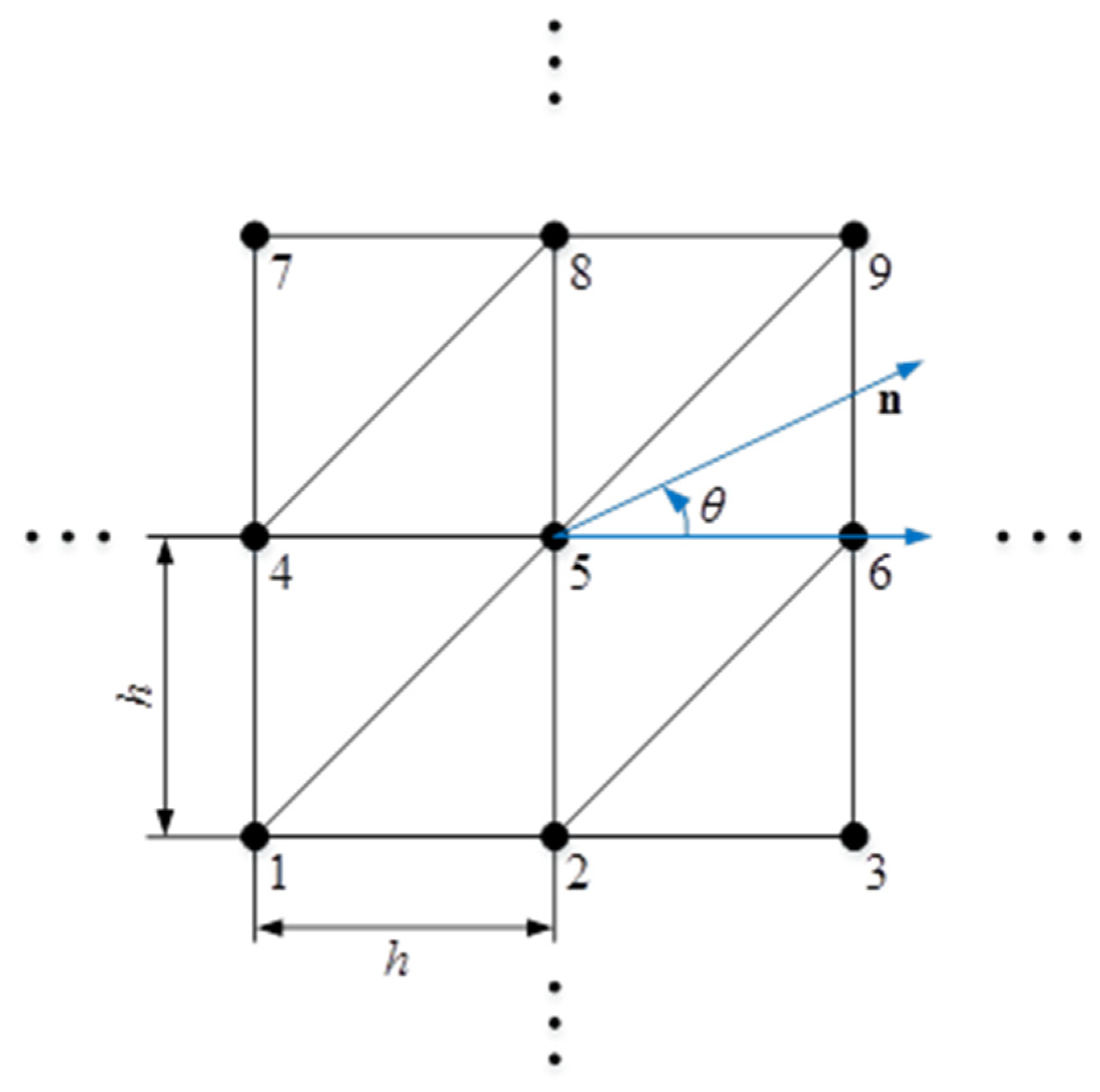
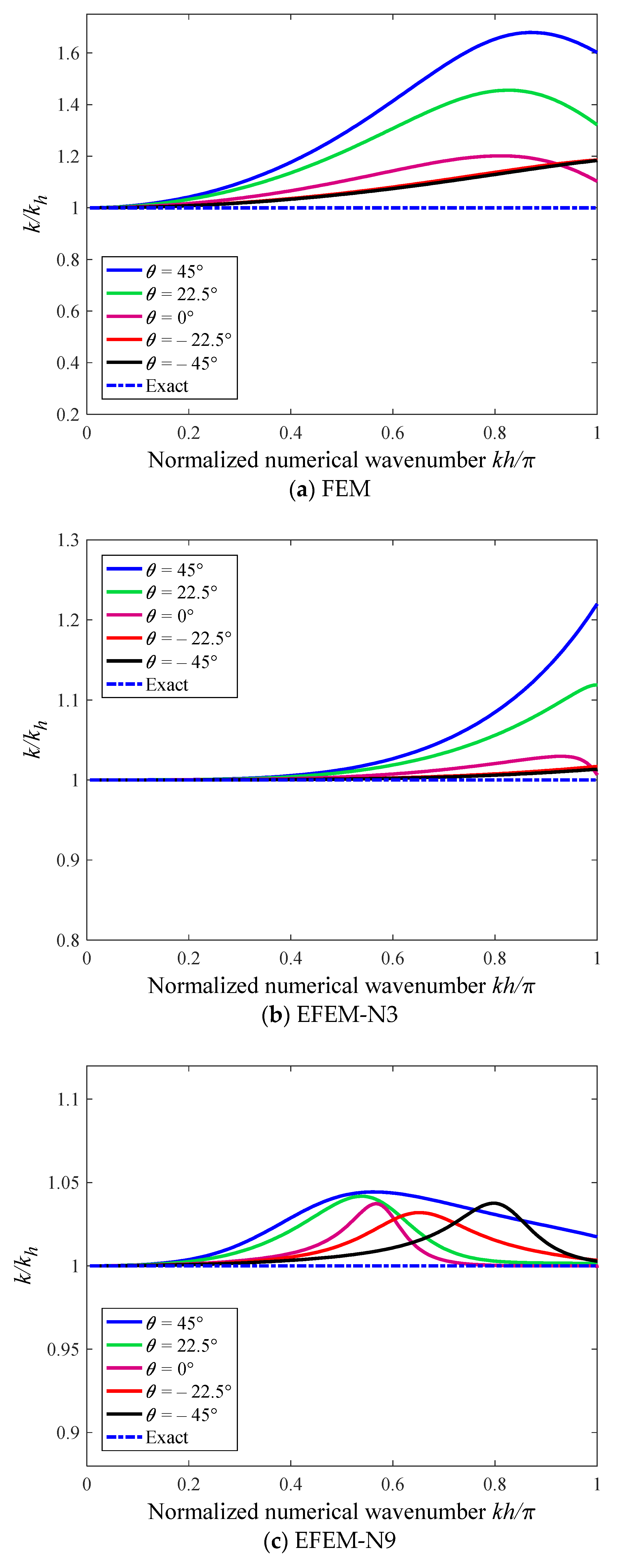
4. Dispersion Analysis

The process of solving elastodynamic problems usually contains two parts, namely, the discretization in the space and time domains. Both of these two parts are able to give rise to considerable numerical errors and affect the solution accuracy of the obtained numerical solutions. In this work, the EFEM was employed for the discretization in the space domain, and the standard implicit Bathe time integration technique was used for the discretization in the time domain. The numerical performance of the different methods in addressing the numerical dispersion error is investigated in this section, and the dispersion errors corresponding to the spatial discretization are firstly studied here.

Assuming that the considered transient wave propagation dynamic problem in this work is time-harmonic, namely, the time-dependent field function variable $u$ can be expressed by:

$$u=U\left(x\right)e^{j\omega t},$$

(13)

in which $j=\sqrt{-1}$, $U\left(x\right)$ is the amplitude distribution of the field function variable $u$; $\omega$ stands for the angular frequency.

Using the above expression, the governing equation in Equation (9) for transient wave propagations can be rewritten as:

$${\nabla }^{2}u+k^{2}u=0,$$

(14)

in which $k=\omega /c$ is the wave number.

Equation (14) is the well-known Helmholtz equation, which is the steady-state form of the governing equation for wave analysis.

Using the constructed field function approximation shown in Equation (5) to discretize Equation (14), we can arrive at the following matrix equation when the additional boundary conditions are not applied:

$$\left(K-k^{2}M\right)U=0,$$

(15)

In two-dimensional space, the general plane wave solution to Equation (15) is $u=A{e}^{jkh\left(x\cos \theta +y\sin \theta \right)}$, and the corresponding numerical solution can be expressed by:

$$u=A{e}^{j{k}_{h}h\left(x\cos \theta +y\sin \theta \right)},$$

(16)

in which $\theta$ stands for the angle of wave travel; $k_h$ and $k$ denote the numerical and exact wave number, respectively.

In Equation (16), $A$ is a vector listing the unknown solution coefficients, which are related to the field function amplitudes for each node. For the present EFEM, the structure of vector $A$ is of the following form [72]:

$$A=\left[\begin{array}{cccc}{A}_1& A_2& \cdots & A_{n_p}, \begin{array}{cccc}{A}_1& A_2& \cdots & \begin{array}{cc}{A}_{n_p},& \cdots \end{array}\end{array}\end{array}\right],$$

(17)

in which $n_p$ is the number of DOFs at one node.

Here, we employed the regular triangular mesh (see Figure 1) to perform the dispersion analysis. By substituting the above expression of the numerical solution into Equation (15), we can obtain:

$$\left[D_{\mathrm{stiff}}-k^2{D}_{\mathrm{mass}}\right]A_i=0,$$

(18)

in which $A_i={\left[\begin{array}{cccc}{A}_1& A_2& \cdots & A_{n_p}\end{array}\right]}^T$ lists the unknown solution coefficients for node $i$; $D_{\mathrm{stiff}}$ and $D_{\mathrm{mass}}$ are the resultant matrices which can be calculated by:

$$\begin{array}{l}{D}_{\mathrm{stiff}}=K_{n,n}+K_{n,n-1}{e}^{-j{k}_{h}h\cos \theta }+K_{n,n+1}{e}^{j{k}_{h}h\cos \theta }+\\ K_{n,n-2}{e}^{j{k}_{h}h\left(\cos \theta -\sin \theta \right)}+K_{n,n+2}{e}^{j{k}_{h}h\left(-\cos \theta +\sin \theta \right)}+\\ K_{n,n-3}{e}^{-j{k}_{h}h\sin \theta }+K_{n,n+3}{e}^{j{k}_{h}h\sin \theta }+\\ K_{n,n-4}{e}^{j{k}_{h}h\left(-\cos \theta -\sin \theta \right)}+K_{n,n+4}{e}^{j{k}_{h}h\left(\cos \theta +\sin \theta \right)}\end{array},$$

(19)

$$\begin{array}{l}{D}_{\mathrm{mass}}=M_{n,n}+M_{n,n-1}{e}^{-j{k}_{h}h\cos \theta }+M_{n,n+1}{e}^{j{k}_{h}h\cos \theta }+\\ M_{n,n-2}{e}^{j{k}_{h}h\left(\cos \theta -\sin \theta \right)}+M_{n,n+2}{e}^{j{k}_{h}h\left(-\cos \theta +\sin \theta \right)}+\\ M_{n,n-3}{e}^{-j{k}_{h}h\sin \theta }+M_{n,n+3}{e}^{j{k}_{h}h\sin \theta }+\\ M_{n,n-4}{e}^{j{k}_{h}h\left(-\cos \theta -\sin \theta \right)}+M_{n,n+4}{e}^{j{k}_{h}h\left(\cos \theta +\sin \theta \right)}\end{array},$$

(20)

If nontrivial solutions to Equation (18) exist, the following relationship is required:

$$\det \left[D_{\mathrm{stiff}}-k^2{D}_{\mathrm{mass}}\right]=0,$$

(21)

From Equations (19) and (20), it is obvious that the numerical wave number $k_h$ is the unique unknown variable in $D_{\mathrm{stiff}}$ and $D_{\mathrm{mass}}$; hence, Equation (21) actually offers the relationship between $k_h$ and $k$. Using Equation (21) for any $k_h$, the corresponding $k$ can be computed by:

$$k=\mathrm{eig}\sqrt{\frac{D_{\mathrm{mass}}}{D_{\mathrm{stiff}}}},$$

(22)

In general, the computed $k$ does not match $k_h$ very well owing to the discretization error in the space domain; in this work, we employed the following indicator to assess the calculated numerical dispersion error from the spatial discretization:

$$\epsilon =\frac{k}{k_h},$$

(23)

For several varying wave travel angles, the numerical dispersion error solutions versus the nondimensional wave number $kh$ from the various numerical techniques are displayed in Figure 2. It should be noted that all of these numerical dispersion errors were computed using a totally identical mesh pattern. It is easy to observe that the computed numerical dispersion errors from the standard FEM were quite large. More importantly, the numerical dispersion errors will become even larger with the increase in the considered nondimensional wave numbers. A similar trend can also be observed in the EFEM-N3 results; however, the numerical dispersion errors from the EFEM-N3 were clearly smaller than those from the FEM. Although the EFEM-N9 is able to offer much smaller numerical dispersion errors than the FEM, its numerical performance in suppressing the numerical dispersion error is still not sufficiently fine, because considerable dispersion errors can still be found with the nondimensional wave number $kh<\mathsf{\pi }$. Among all of the considered numerical techniques, the performance of the EFEM-N6 in suppressing the numerical dispersion from the spatial discretization is the best, because almost no dispersion errors from the discretization in the space domain can be seen for the considered nondimensional wave number. More importantly, the numerical dispersion errors from the EFEM-N6 were very close to zero in all considered wave travel angles, namely, the numerical anisotropy issue also can be largely alleviated by the present EFEM-N6, while this intractable phenomenon can clearly be seen in the results from the other mentioned numerical techniques (i.e., FEM, EFEM-N3 and EFEM-N9). These findings indicate that the present EFEM with the quadric polynomial enrichment functions is basically sufficient to generate adequately small numerical dispersion errors for the wave analysis. Though more accurate solutions, indeed, can be yielded when the higher order of the polynomial bases are employed to create the enrichment functions, more computational expenses are also required. To reduce the computational efforts as much as possible, in this work we only considered the enrichment functions that are created by linear and quadric polynomial bases.

Apart from the discretization in the space domain, the discretization in the time domain is also a major source that produces numerical errors in solving elastodynamic problems. Here, the numerical error affected by the time integration scheme was also taken into consideration in the dispersion analysis.

Owing to the fact that the recently developed Bathe implicit temporal discretization technique always shows very excellent numerical features in handling linear and nonlinear structural dynamic problems, in this work the standard Bathe was employed for the discretization in the time domain. In the standard Bathe method, the following assumptions are employed:

$$\{\begin{array}{l}{}^{t+\Delta t/2}\dot{u}={}^t\dot{u}+\frac{\Delta t}{4}\left({}^t\ddot{u}+{}^{t+\Delta t/2}\ddot{u}\right)\\ {}^{t+\Delta t/2}u={}^{t}u+\frac{\Delta t}{4}\left({}^t\dot{u}+{}^{t+\Delta t/2}\dot{u}\right)\\ {}^{t+\Delta t}\dot{u}=\frac{1}{\Delta t}{}^{t}u-\frac{4}{\Delta t}{}^{t+\Delta t/2}u+\frac{3}{\Delta t}{}^{t+\Delta t}u\\ {}^{t+\Delta t}\ddot{u}=\frac{1}{\Delta t}{}^t\dot{u}-\frac{4}{\Delta t}{}^{t+\Delta t/2}\dot{u}+\frac{3}{\Delta t}{}^{t+\Delta t}\dot{u}\end{array},$$

(24)

Using the assumptions in the above equation to the discretize matrix equation shown in Equation (12) and following the similar steps in References [72,73,74,75], the total dispersion error in the elastodynamic analysis can be expressed by:

$$\frac{c_h}{c}=\frac{{\omega }_h/k_h}{c}=\frac{{\omega }_h\Delta t}{k_{h}c\Delta t}=\frac{{\omega }_h\Delta t}{k_{h}h\mathrm{CFL}}=\frac{f\left(\omega \Delta t\right)}{k_{h}h\mathrm{CFL}}=\frac{f\left(kh\mathrm{CFL}\right)}{k_{h}h\mathrm{CFL}},$$

(25)

in which $c$ stands for the wave speed; the subscript $h$ means that the corresponding variables are from the numerical solutions; $\Delta t$ denotes the interval of temporal discretization; CFL represents the Courant–Friedrichs–Lewy number, which is defined by CFL = $c\Delta t/h$; $f\left(\right)$ is a defined function with respect to the parameter $k_{h}h\mathrm{CFL}$.

Using the Taylor series expansion, Equation (25) can be rewritten by:

$$\begin{array}{l}\frac{c_h}{c}=\frac{{\omega }_h/k_h}{c}=\frac{{\omega }_h\Delta t}{k_{h}c\Delta t}=\frac{{\omega }_h\Delta t}{k_{h}h\mathrm{CFL}}=\frac{f\left(kh\mathrm{CFL}\right)}{k_{h}h\mathrm{CFL}}\\ =\frac{1}{k_{h}h\mathrm{CFL}}\left[f\left(0\right)+f^{\prime }\left(0\right)\left(kh\mathrm{CFL}\right)+\frac{f^{″}\left(0\right)}{2!}{\left(kh\mathrm{CFL}\right)}^2+\cdots \right],\\ =\frac{k}{k_h}\left(1-\frac{1}{24}{\left(kh\mathrm{CFL}\right)}^2+\frac{61}{17280}{\left(kh\mathrm{CFL}\right)}^4+\cdots \right) \end{array}$$

(26)

From Equation (25), we also can obtain

$$\frac{c_h}{c}=\frac{{\omega }_h/k_h}{c}=\frac{{\omega }_h/k_h}{\omega /k}=\frac{k}{k_h}\frac{{\omega }_h}{\omega }=\frac{k}{k_h}\frac{T}{T_h},$$

(27)

in which $T$ stands for the period of one considered wave mode.

By comparing Equations (26) and (27), the total numerical error in the elastodynamic analysis can be expressed in the following form:

$$\frac{c_h}{c}=\frac{k}{k_h}\frac{T}{T_h}=\frac{k}{k_h}\underset{\mathrm{Temporal} \mathrm{dispersion} \mathrm{error} T/T_h}{\underbrace{\left(1-\frac{1}{24}{\left(kh\mathrm{CFL}\right)}^2+\frac{61}{17280}{\left(kh\mathrm{CFL}\right)}^4+\cdots \right)}},$$

(28)

From Equations (25)–(28), it is very interesting to observe that both the discretizations in the space and time domains are able to result in numerical errors in the final numerical solutions for the elastodynamic analysis. The first term in Equation (27) is the defined indicator to assess the spatial discretization error. From the above formulation and analysis, it is seen that the error $k/k_h$, indeed, mainly comes from the discretization in the space domain, and it is determined by the used field function approximation in the space domain. The second term $T/T_h$ in Equation (27) represents the additional effects from the temporal discretization, and it is closely associated with the employed the time integration scheme. In this work, the standard Bathe method was exploited for the temporal discretization, and it has been proved that $T/T_h$ is actually a monotonic function with respect to the nondimensional temporal discretization interval CFL. Therefore, the total numerical error can be continuously decreased by reducing the used CFL numbers as long as the spatial discretization error $k/k_h$ is adequately small; then, the so-called monotonic convergence property can be reached. From the previous analysis, it is seen that the EFEM-N6 can basically meet this requirement, while the other mentioned numerical techniques (i.e., FEM, EFEM-N3 and EFEM-N9) cannot generate adequately small spatial discretization errors. In the next section, several supporting numerical experiments are conducted to verify that the present EFEM-N6 with the Bathe method, indeed, possesses the important monotonic convergence property with respect to the nondimensional temporal discretization step CFL, while the other numerical approaches do not have this very valuable numerical feature.

5. The Implementation of the EFEM for the Transient Wave Analysis

From the above formulation, we can find that the implementation of the present EFEM is quite similar to the standard FEM in solving transient wave propagations, and the general procedure mainly consists of the following steps:

(1) Perform the required spatial discretization using the standard mesh as in the FEM. In general, the triangular elements and tetrahedron elements are employed for two-dimensional and three-dimensional problems, respectively.

(2) Create the required field function approximation for the considered problem. In creating the numerical approximation, compared to the standard FEM, more unknown coefficients for each node are involved in the local interpolation, and various basis functions can be employed for the local numerical approximation.

(3) Assemble the system mass and stiffness matrices. In this step, the required numerical integration is still performed using the Gauss integration rule. However, the scale of the obtained system matrices will be clearly larger than those from the standard FEM, because more unknowns are involved for each node.

(4) Remove the possible linear dependence of the obtained matrix equation. Note that linear dependent nodal shape functions are possibly employed to construct the required field function approximation; then, the linear dependent matrix equation will be generated. For stable and reliable numerical solutions, extra numerical treatments are required to remove the possible linear dependence of the obtained matrix equation.

(5) Impose the involved boundary conditions and perform the required temporal discretization. Usually, direct time integration techniques are employed to perform the required time integration. This step is almost the same as in the standard FEM.

(6) Solve the finally obtained matrix equation and assess the obtained numerical results; this process is also quite similar as in the standard FEM.

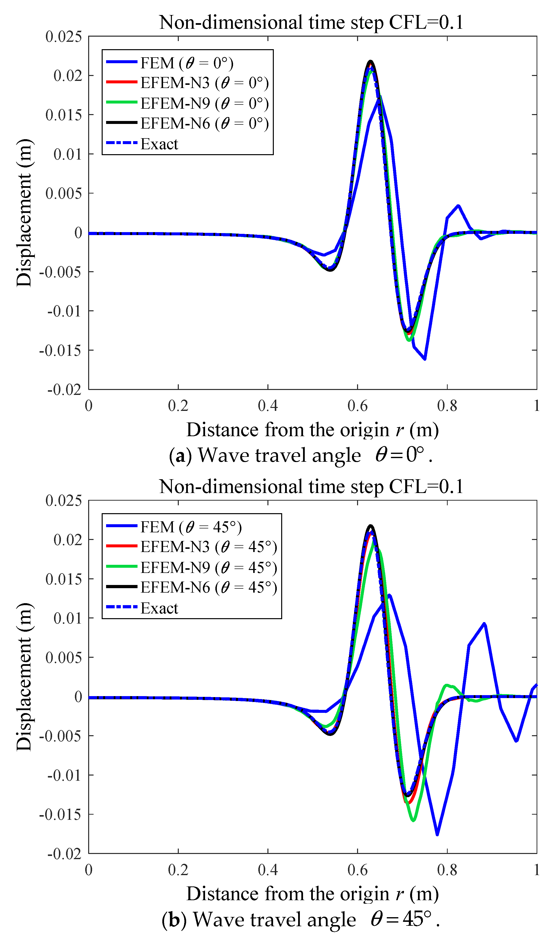
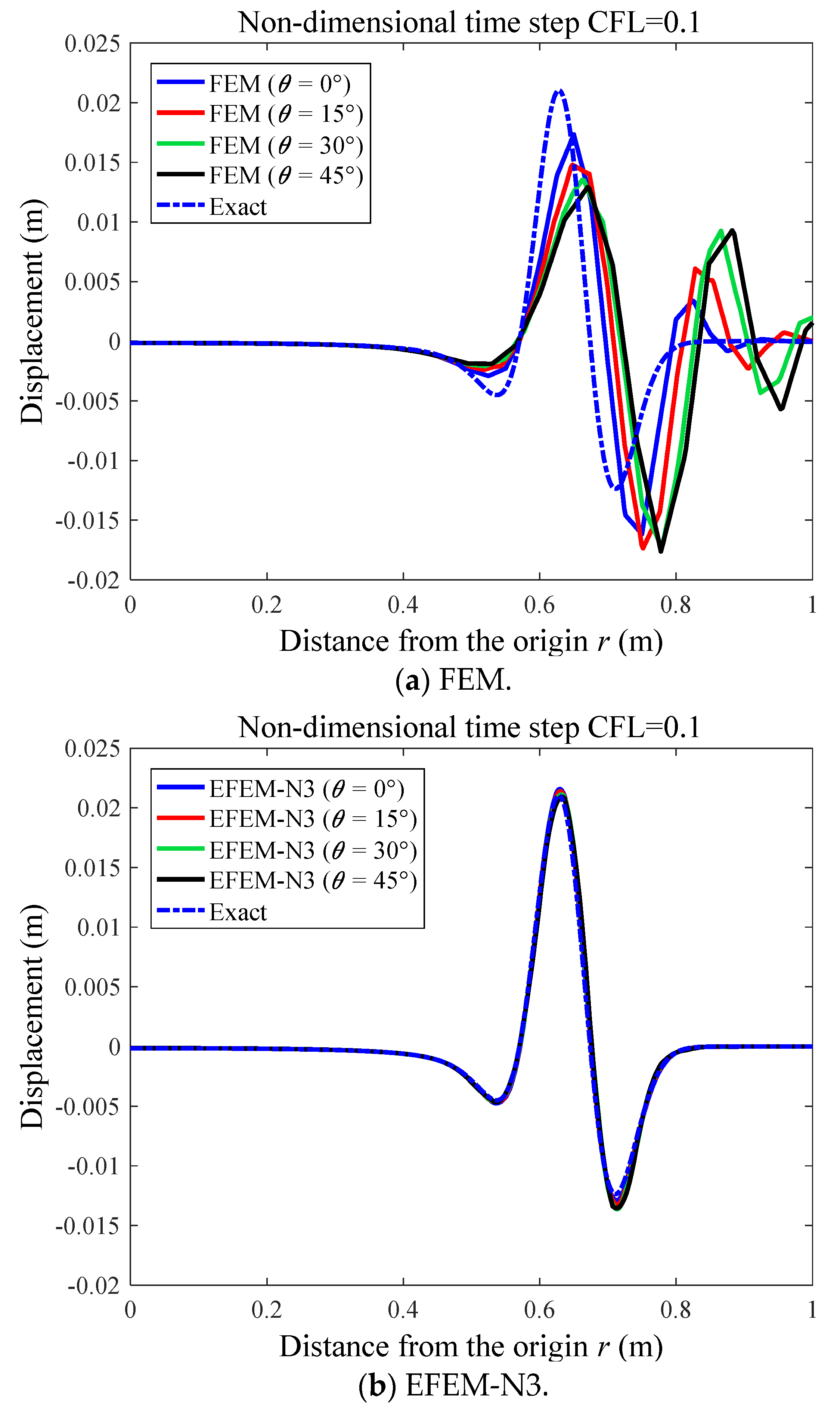
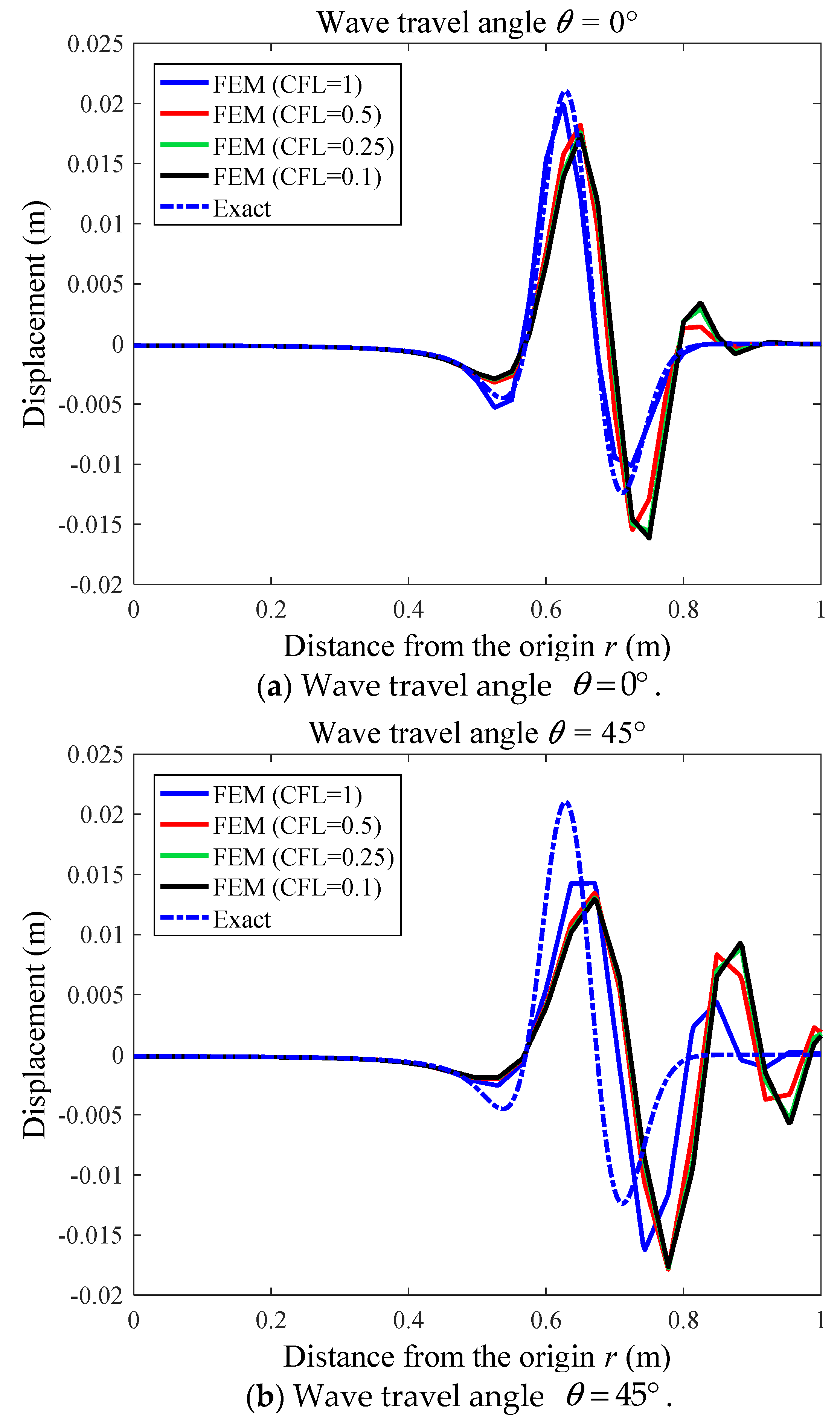
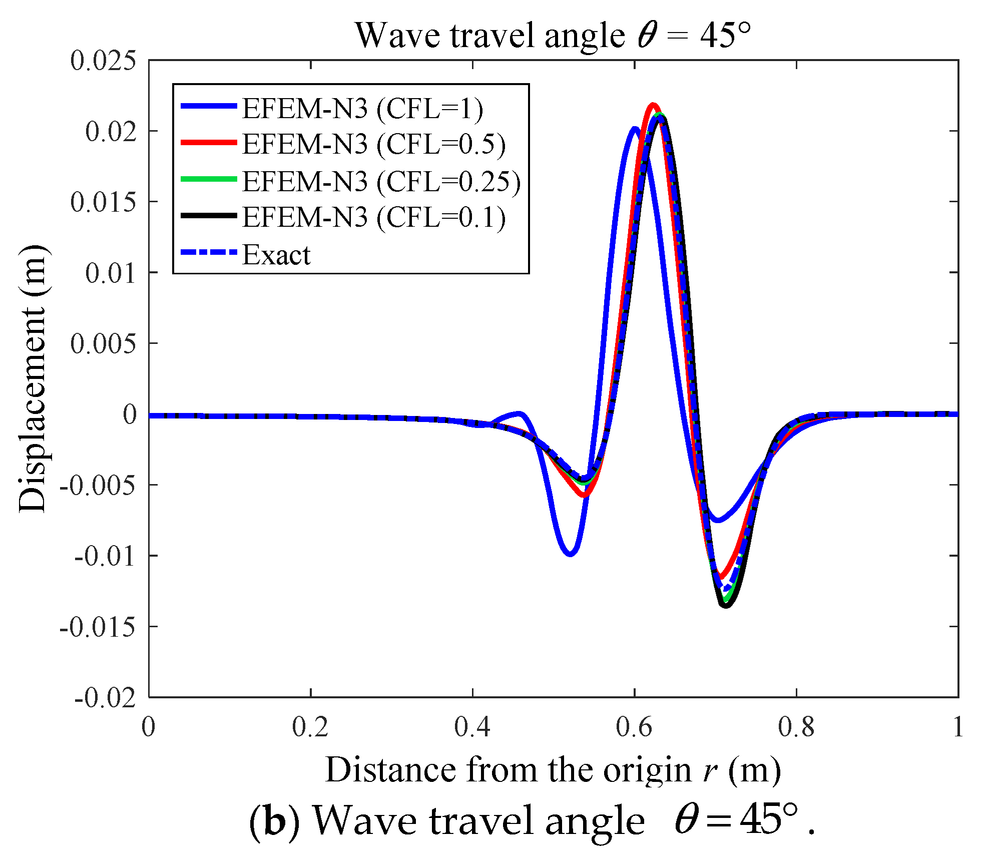
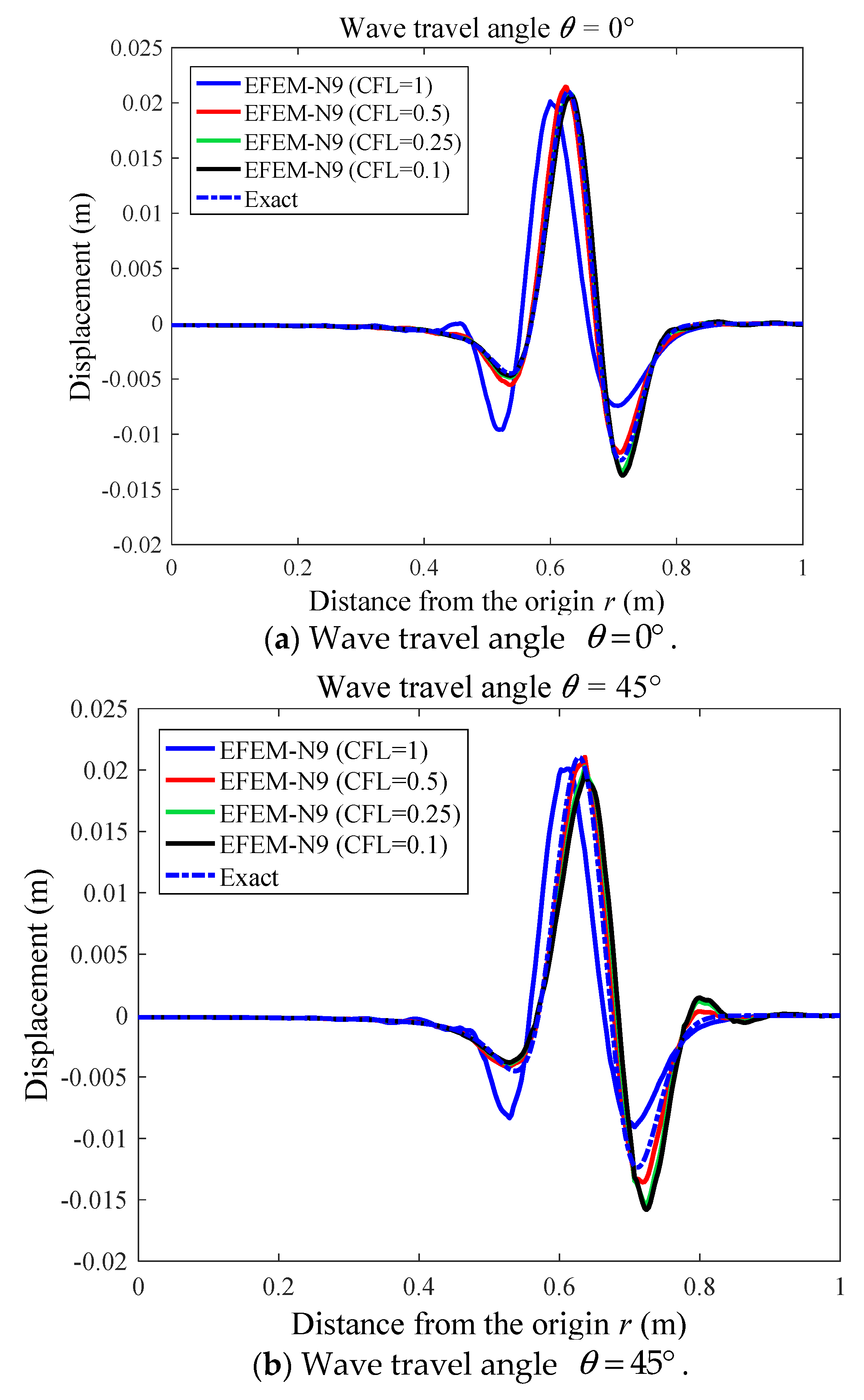
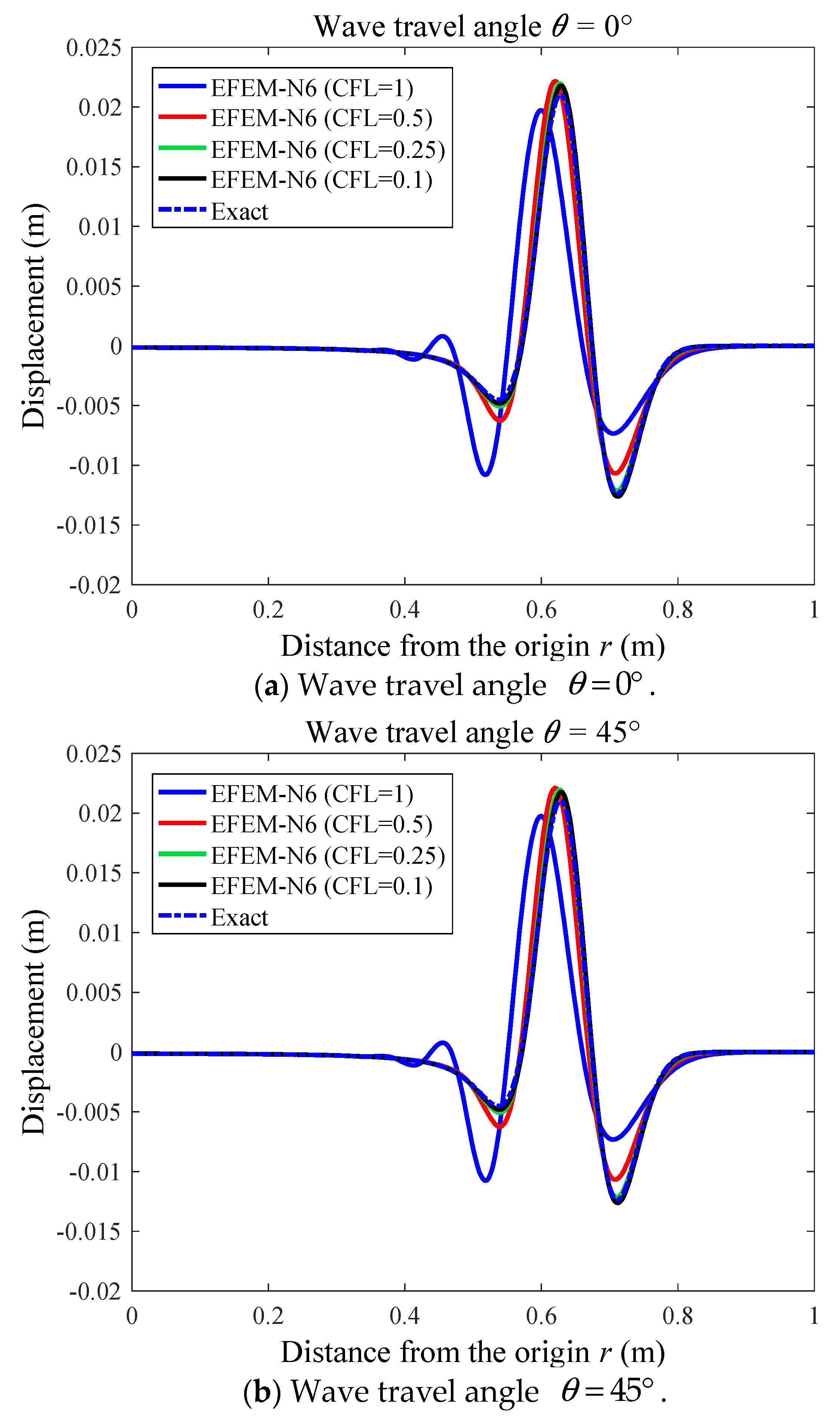
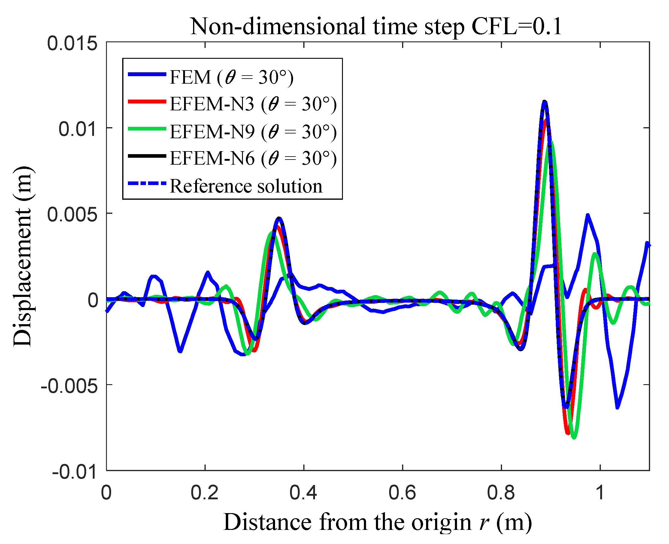
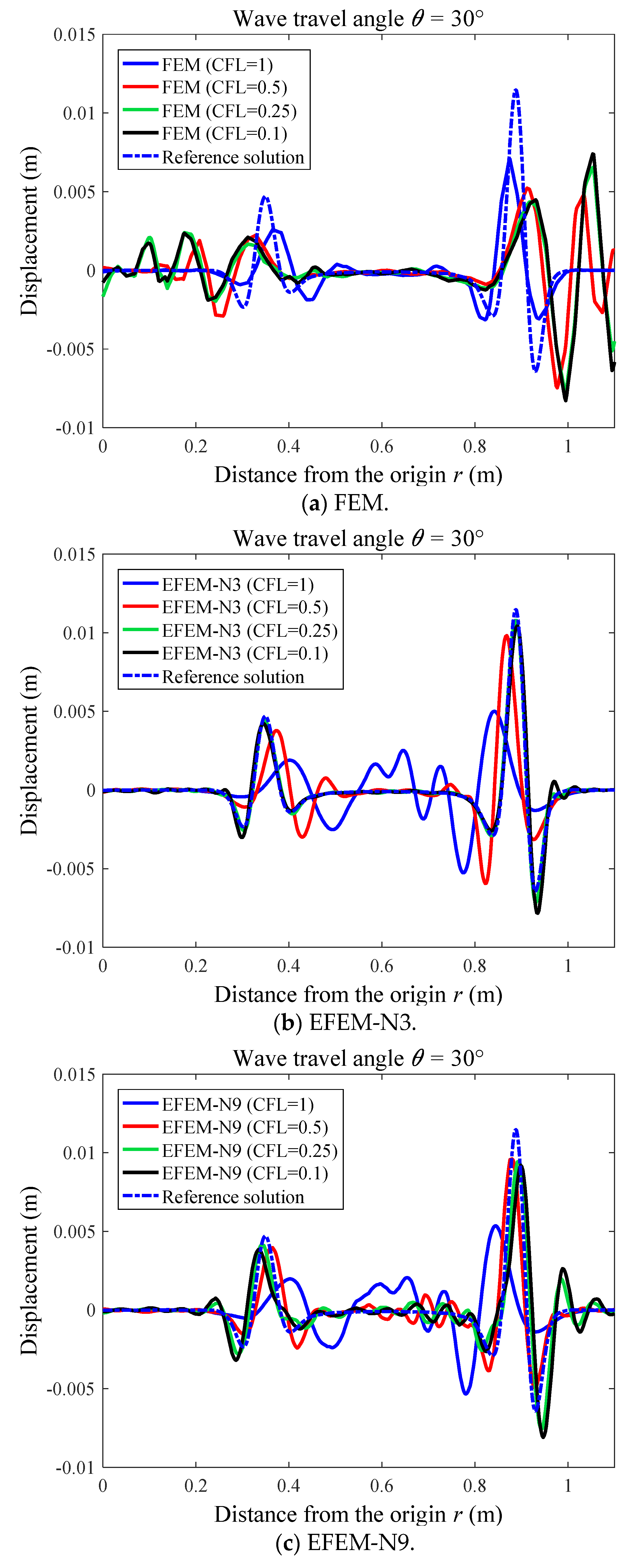
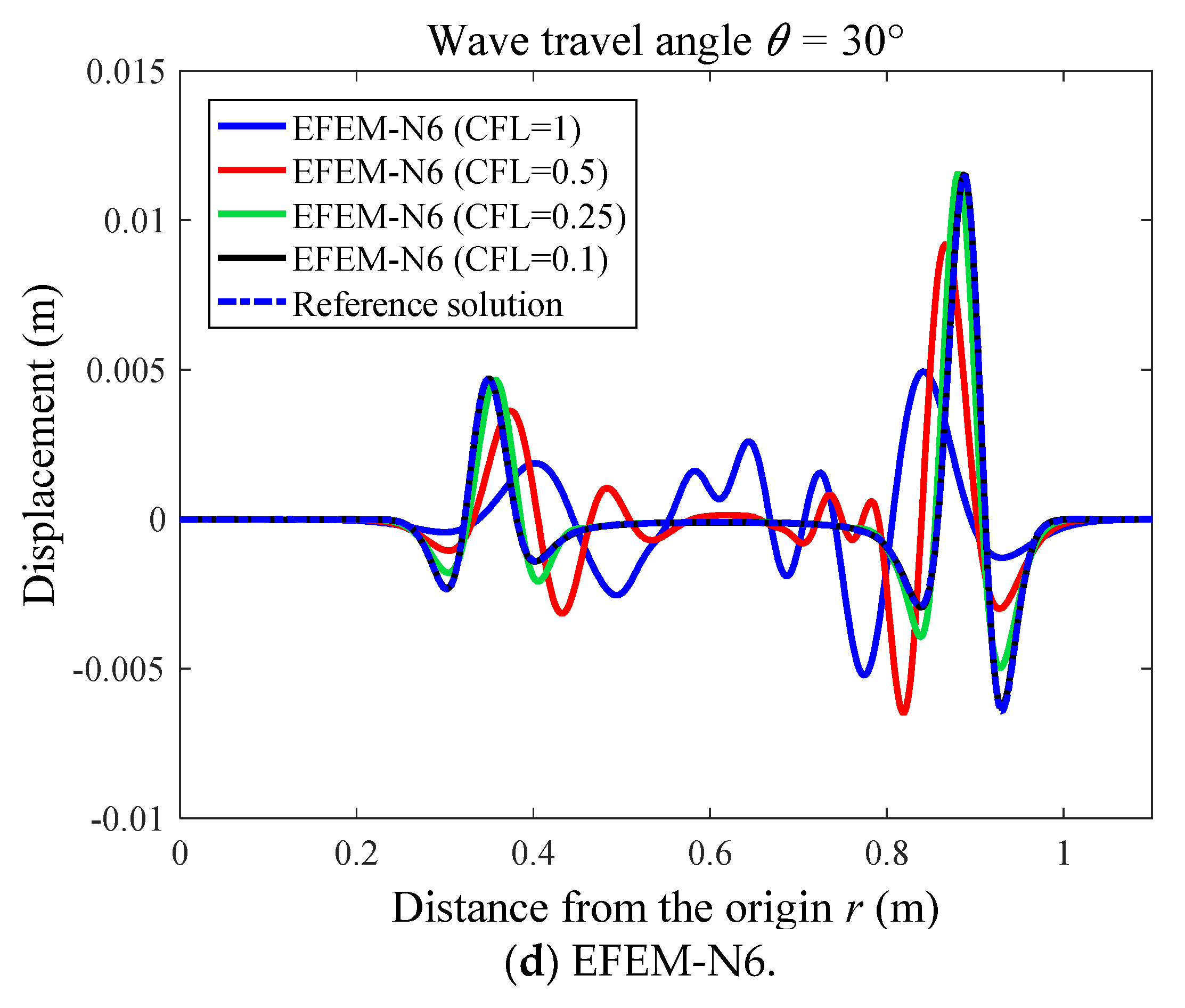
6. Numerical Example

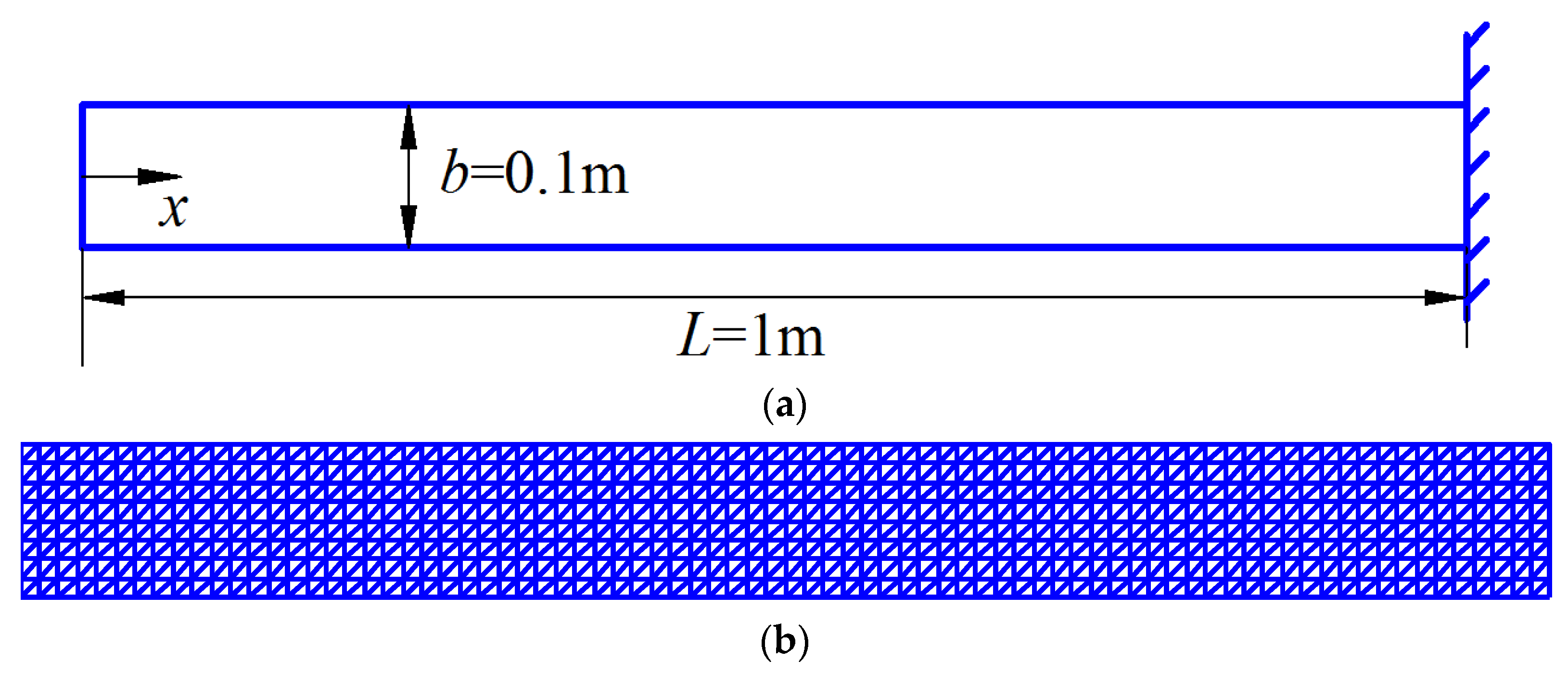
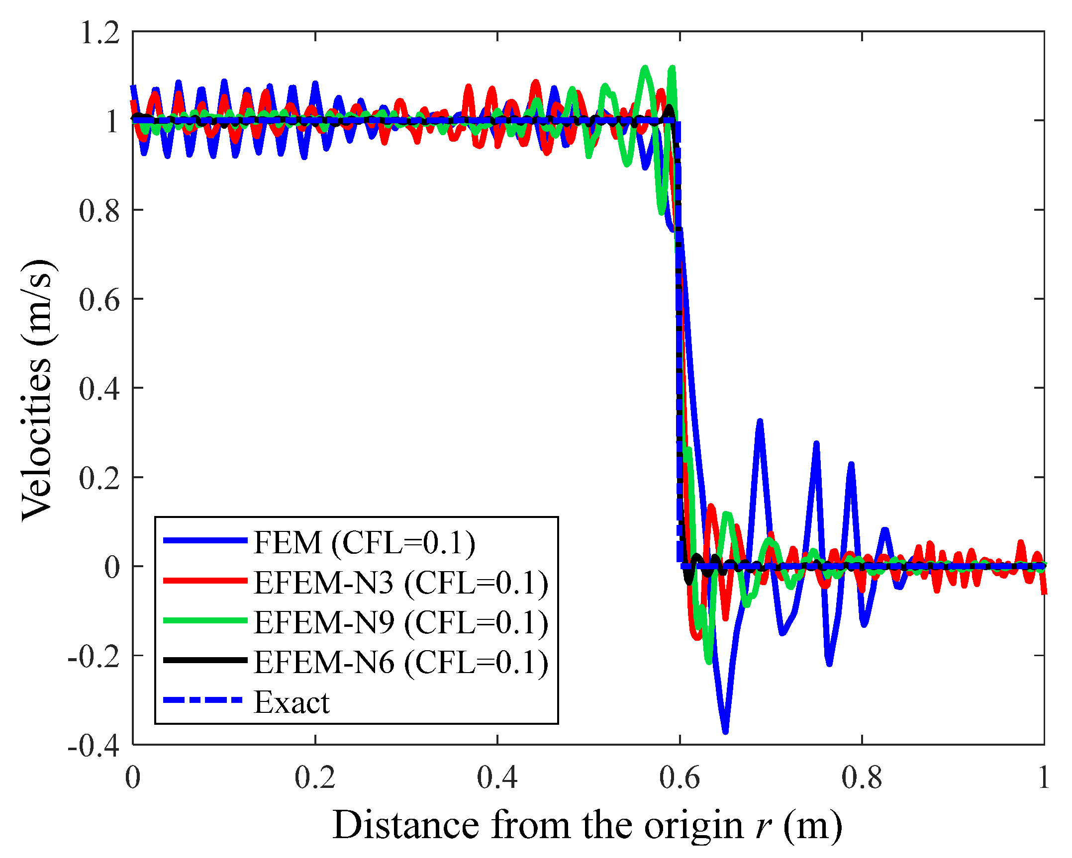
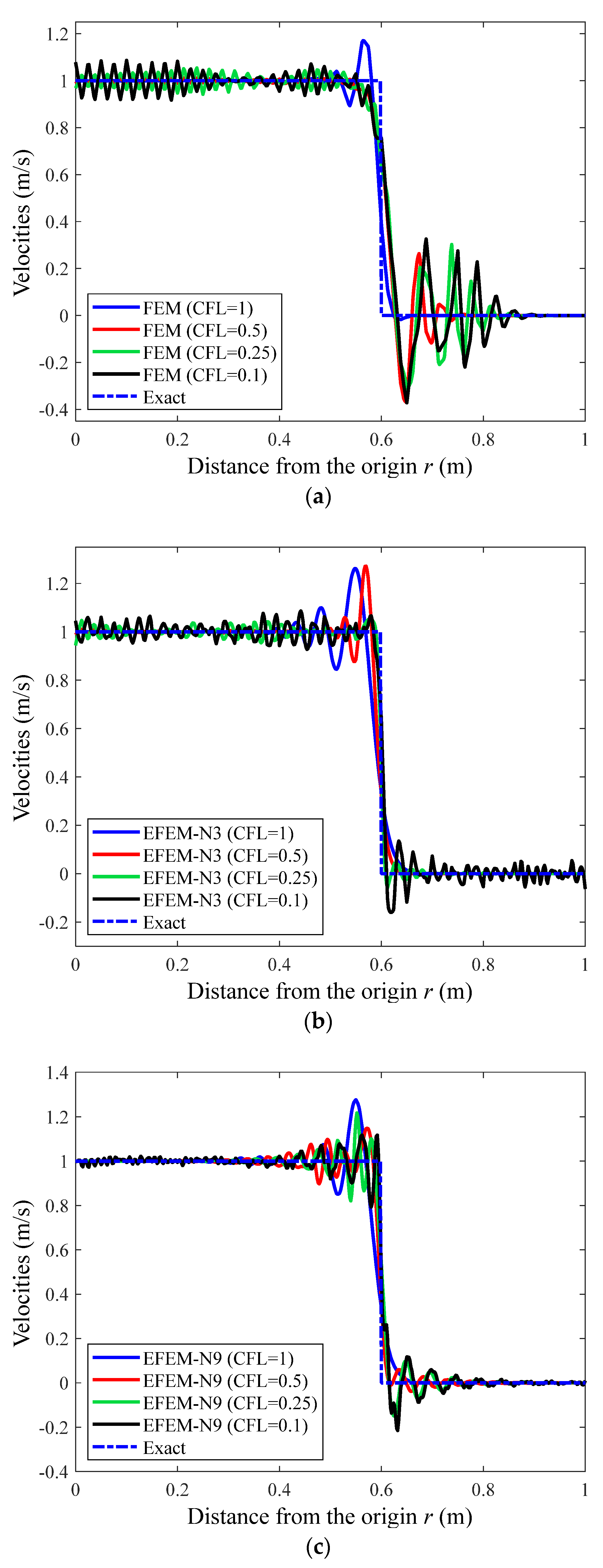
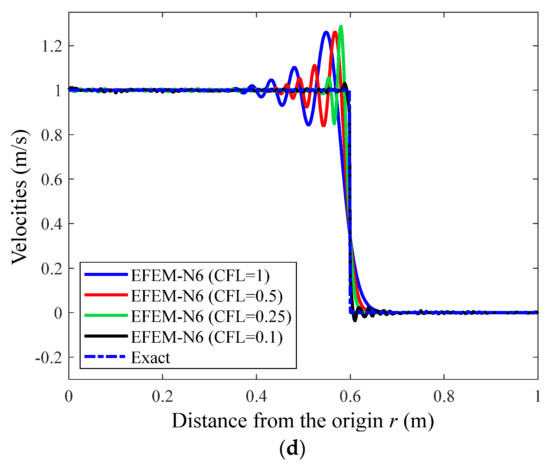
6.1. The Scalar Wave Propagation in a Clamped-Free Elastic Bar

We firstly consider the transient scalar wave propagation in an elastic bar with a length L = 1 m and width b = 0.1 m. The left end of this elastic bar is free, and the other end is clamped (see Figure 3a). The considered wave travel speed in this bar is c = 1 m/s. To solve this problem, the required discretization in the space domain is accomplished by using the uniform triangular mesh with the node interval h = 0.0125 m (see Figure 3b). This transient wave propagation problem is excited by using the following initial conditions:

$$u\left(x,t=0\right)= 0 \mathrm{m},\dot{u}\left(x,t=0\right)=0 \mathrm{m}/\mathrm{s},\dot{u}\left(x,t>0\right)=1 \mathrm{m}/\mathrm{s},,$$

(29)

in which $u$ denotes the considered displacement variable, and the overdot stands for the time derivative.

The computed velocity distributions of this elastic bar were employed to investigate this simple transient wave propagation problem. For the nondimensional temporal discretization step CFL = 0.1 and the considered time point t = 0.6 s, the calculated velocity distributions of this elastic bar from various numerical approaches together with the exact solutions are displayed in Figure 4. It is seen from the figure that the numerical solution from the standard FEM was not sufficiently accurate, and many unwanted peaks can be found in the solutions. In contrast to the standard FEM, the EFEM-N3 and EFEM-N9 are able to generate more accurate solutions despite several relatively small spurious peaks that can still be seen in the solutions. Among all of the considered numerical approaches, the numerical performance of the proposed EFEM-N6 is the best, since the resultant numerical solutions of the velocity distributions agreed very well with the exact solutions, and almost no spurious peaks can be seen in the solutions.

Furthermore, this numerical experiment was studied by exploiting the varying nondimensional time integration steps (CFL = 1, CFL = 0.5, CFL = 0.25 and CFL = 0.1), and the relevant computed velocity distributions are plotted in Figure 5. Here, the abovementioned four different numerical approaches were again employed, and the considered time point was still t = 0.6 s. By carefully comparing the computed velocity distributions shown in Figure 5, we can observe that the present EFEM-N6 has the ability to continuously increase the solution accuracy by employing the decreasing nondimensional time integration steps, because the EFEM-N6 solutions will converge to the exact solutions when the employed CFL numbers become smaller. On the contrary, the EFEM-N3, EFEM-N6 and the standard FEM do not have this ability, because the corresponding velocity distributions can become unexpectedly worse when decreasing CFL numbers are utilized for time integration. These observations can be broadly explained by two factors; one factor is that the EFEM-N6 can produce close-to-zero spatial discretization errors, while the corresponding spatial discretization errors from the other three numerical approaches are relatively large (See Figure 2); the other factor is that the additional numerical error from the time integration is actually a monotonic decreasing function of the nondimensional time integration steps. These two factors can ensure that the EFEM-N6 has the monotonic convergence property in the transient wave analysis. From the above analysis, it is demonstrated that the numerical performance of the EFEM-N6 clearly outperforms the other three numerical approaches in solving transient wave propagations.

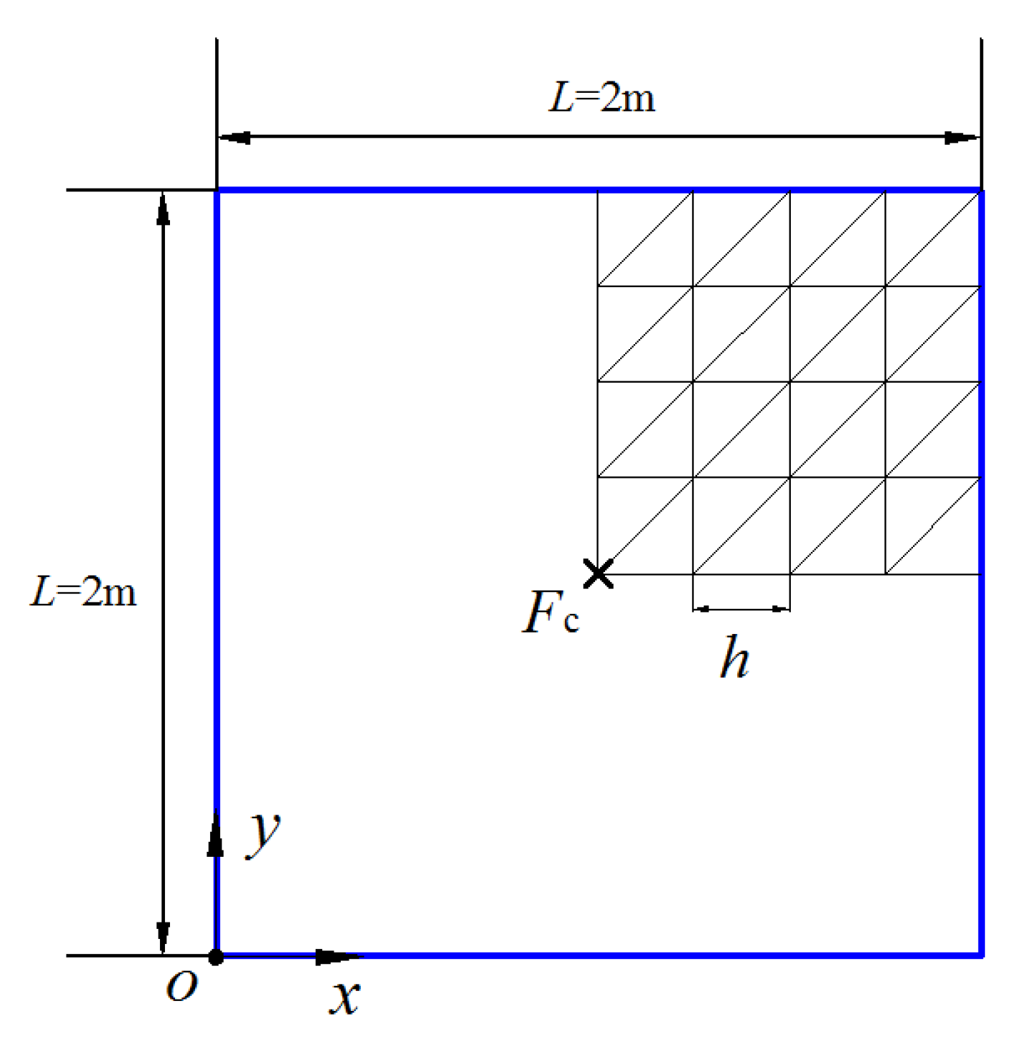
6.2. The Scalar Wave Propagation in a Square Pre-Stressed Membrane

The numerical experiment on scalar wave propagation in a two-dimensional square pre-stressed membrane is investigated in this section. The geometric configuration of the problem domain is sketched in Figure 6, and the wave speed for this numerical experiment was c = 1 m/s. We employed a regular mesh pattern with a nodal interval h = 0.025 m to discretize the membrane. The point load was at the middle of the square domain, and the excitation load was of the following Ricker wavelet form [72,73]:

$$F_c=0.5\left[1-2{\mathsf{\pi }}^2{f}_s^2{\left(t-t_s\right)}^2\right]\exp \left[-{\mathsf{\pi }}^2{f}_s^2{\left(t-t_s\right)}^2\right],$$

(30)

in which $t_s$ = 0.25 s and $f_s$ = 5 Hz stand for the time and frequency parameters.

Considering the symmetry feature of this numerical experiment, in practical computation processes, only the partial problem domain is needed to model (see Figure 6). Here, the transient displacement responses from the different numerical techniques were examined. When the nondimensional time step CFL = 0.1 and the time point t = 0.9 s were chosen, the displacement responses along two disparate angles ($\theta =0°$ and $\theta =45°$) are depicted in Figure 7. Note that the exact solution to this problem is available; hence, it is also plotted in the figures. It can be observed that the amount of numerical error in the FEM solutions is quite large. Though the EFEM-N3 and EFEM-N9, indeed, can suppress the numerical error to some degree, the EFEM-N6 solutions are the most accurate. These findings indicate that the use of quadric polynomials as an enrichment function is more effective than the linear polynomial and first order of the trigonometric function to control the amount of numerical error for the wave analysis.

Furthermore, the numerical analysis of the problem was performed by considering the varying angles, and the related displacement responses at the time point t = 0.9 s from various methods are displayed in Figure 8. It is clear that the varying angles can visibly affect the accuracy of the solutions from FEM, EFEM-N3 and EFEM-N9, namely, the so-called numerical anisotropy issue can be obviously seen, while the EFEM-N6 solutions are almost insensitive to the angles, and very reliable solutions can still be yielded for all considered angles.

In more detail, several varying nondimensional time step CFL numbers were considered here to perform an overall analysis of this numerical experiment. Similar to the previous discussion, for two disparate angles ($\theta =0°$ and $\theta =45°$), the displacement responses at the time point t = 0.9 s from the various methods are given in Figure 9, Figure 10, Figure 11 and Figure 12. These figures show that the FEM, EFEM-N3 and EFEM-N9 always failed to continuously increase the solution quality by decreasing the employed CFL numbers, namely, the monotonic convergence property for the transient wave analysis cannot be achieved. On the contrary, it is very interesting to find that the EFEM-N6 basically has the monotonic convergence property, and the corresponding numerical solutions will become more accurate when the employed CFL number becomes smaller. A possible cause for these observations is that the EFEM-N6 can produce adequately small spatial dispersion errors, while the errors from other methods are relatively large, which have been seen in the dispersion analysis. With this good numerical feature, the present EFEM-N6 obviously has stronger abilities than the other numerical techniques in handling very complicated wave propagations in practice.

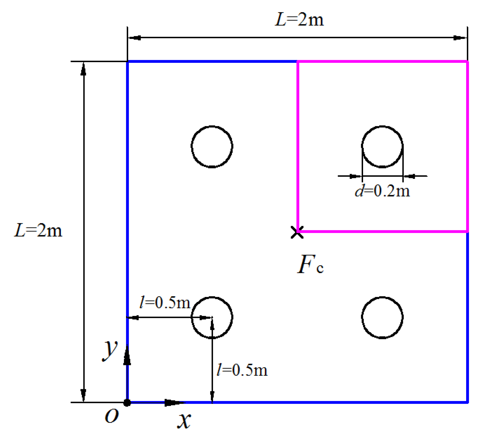
6.3. The Scalar Wave Propagation in a Membrane with Holes

In the last numerical experiment, we still consider the scalar wave propagation with a wave speed c = 1 m/s in a square pre-stressed membrane, while in this case the membrane had several evenly placed holes (see Figure 13). Similar to the previous numerical experiment, only the partial problem domain was needed to model this problem, owing to the symmetry feature. The triangular mesh pattern with an average nodal interval h = 0.02 m was employed here. The point load at the middle of this membrane was still a Ricker wavelet with an amplitude A = 0.4 N, time parameter $t_s$ = 0.1 s and frequency parameter $f_s$ = 10 Hz.

With a wave travel angle $\theta =30°$, nondimensional temporal discretization interval CFL = 0.1 and time point t = 1 s, Figure 14 displays the displacement distribution responses using various numerical techniques. With the aim to examine the accuracy of the obtained solutions, the reference solution from the commercial software package ABAQUS with very refined mesh is also presented here to investigate this numerical experiment. Figure 14 shows very good agreements of the EFEM-N6 solutions with the reference ones, while the other three methods clearly failed to yield very accurate solutions.

Additionally, we also perform the numerical analysis of this wave problem by employing the varying nondimensional temporal discretization intervals and the related displacement distribution responses are shown in Figure 15. Here the wave travel angle $\theta =30°$. It is again confirmed from these figures that the proposed EFEM-N6 can yield monotonic convergence solutions when the CFL number trends to zero, while the other three methods obviously did not exhibit this good numerical feature. As discussed and analyzed in the previous sections, this good numerical feature can be obtained because the EFEM-N6 can yield sufficiently small numerical dispersion errors in the space domain discretization, while the related errors from the other methods were relatively large.

6.4. Study on the Computational Cost

From the previous three numerical experiments, we can clearly obtain that the proposed EFEM-N6 showed much more excellent numerical performance than the other three mentioned numerical approaches (i.e., FEM, EFEM-N3 and EFEM-N9) for the analysis of transient wave propagationsm and the close-to-exact numerical solutions can be generated by utilizing the decreasing time integration steps. However, the detailed computational cost of the different numerical approaches in solving the transient wave propagations has still not been taken into consideration so far. In this section, the computational cost and the computational efficiency of all of the considered numerical approaches is investigated in great detail. To comprehensively and fairly compare the obtained results, the identical meshes and the following relative error norm was used to measure the accuracy of the obtained numerical solutions.

$$e_r=\sqrt{\frac{{\displaystyle {\int }_V{\left(u_e-u_h\right)}^2\mathrm{d}V}}{{\displaystyle {\int }_V{u}_e{}^2\mathrm{d}V}}},$$

(31)

in which $V$ denotes the involved total problem domain; $u_e$ and $u_h$ represent the exact and numerical solutions, respectively.

For a series of varying nondimensional time integration steps (CFL = 1, CFL = 0.5, CFL = 0.25 and CFL = 0.1), the detailed computational cost, which is represented by the CPU time (s) and the relative error results from the different numerical approaches in solving the previous two numerical experiments with exact solutions are given in

Table 1. Comparisons of the computational cost and computational efficiency of the different numerical approaches in solving the scalar wave propagation in a clamped-free elastic bar.

Methods	Number of DOFs	Nonzero Entities in the System Matrices	CPU Time for Spatial Discretization (s)	Nondimensional Time Steps	CPU Time for Temporal Discretization (s)	Total CPU Time (s)	Total Numerical Error (%)
FEM-T3	729	3465	0.66	CFL = 1	2.63	3.29	7.16
				CFL = 0.5	5.36	6.02	11.51
				CFL = 0.25	9.52	10.18	12.69
				CFL = 0.1	13.32	13.98	13.14
EFEM-N3	2187	41411	2.64	CFL = 1	9.75	12.39	11.14
				CFL = 0.5	16.57	19.21	8.28
				CFL = 0.25	29.03	31.67	5.09
				CFL = 0.1	54.35	56.99	7.12
EFEM-N9	6561	382975	7.65	CFL = 1	19.21	26.86	11.01
				CFL = 0.5	34.21	41.86	6.53
				CFL = 0.25	54.38	62.03	6.68
				CFL = 0.1	95.48	103.13	7.32
EFEM-N6	4374	169496	4.16	CFL = 1	13.26	17.42	11.16
				CFL = 0.5	22.01	26.17	8.45
				CFL = 0.25	36.13	40.29	5.43
				CFL = 0.1	65.93	70.09	2.01

and

Table 2. Comparisons of the computational cost and computational efficiency of different numerical approaches in solving the scalar wave propagation in a square pre-stressed membrane.

Methods	Number of DOFs	Nonzero Entities in the System Matrices	CPU Time for Spatial Discretization (s)	Nondimensional Time Steps	CPU Time for Temporal Discretization (s)	Total CPU Time (s)	Total Numerical Error (%)
FEM-T3	1681	8241	1.49	CFL = 1	7.03	8.52	52.33
				CFL = 0.5	10.55	12.04	87.73
				CFL = 0.25	20.19	21.68	95.38
				CFL = 0.1	37.84	39.33	97.31
EFEM-N3	5043	99751	11.68	CFL = 1	13.77	25.45	59.39
				CFL = 0.5	24.23	35.91	39.89
				CFL = 0.25	43.62	55.3	11.95
				CFL = 0.1	82.19	93.87	19.69
EFEM-N9	15129	923,343	37.89	CFL = 1	41.28	79.17	51.29
				CFL = 0.5	81.62	119.51	13.82
				CFL = 0.25	147.82	185.71	19.54
				CFL = 0.1	347.38	385.27	22.76
EFEM-N6	10086	408614	29.62	CFL = 1	27.16	56.78	60.85
				CFL = 0.5	47.71	77.33	22.57
				CFL = 0.25	89.93	119.55	9.41
				CFL = 0.1	208.58	238.2	3.26

. In this work, all the numerical computations were performed using a laptop with a single core Intel 2.2 GHz CPU and 2 GB RAM. From the tables, the following valuable points can be observed:

(1) When the identical mesh patterns were employed, the number of required degree of freedoms (DOFs) and nonzero entities in the system matrices from the standard FEM were much larger than that of the proposed EFEM. This was because more nodal unknowns for each node were employed to construct the required field function approximation in the EFEM.

(2) Compared to the standard FEM, in the transient wave analysis the required computational cost for the EFEM was much more expensive. As a result, the computational efficiency of the EFEM was clearly lower than the standard FEM.

(3) For the three considered EFEMs (i.e., EFEM-N3, EFEM-N6 and EFEM-N9), more additional nodal unknowns were involved for each node, and the obtained EFEM will be more numerically expensive, leading to the lower computation efficiency in the transient wave analysis.

(4) In solving transient wave propagations using numerical approaches, the total required computational cost mainly consisted of two different parts, namely, the CPU time for the spatial and temporal discretizations, respectively. Additionally, it was also clear that the required computational cost for the temporal discretization was much more expensive than that for the spatial discretization.

(5) When the standard FEM was employed for the transient wave analysis, the relative numerical error did not become lower for the smaller used nondimensional time integration steps. As discussed in the previous text, this was because the standard FEM cannot provide sufficiently low spatial discretization errors. Likewise, very similar observations can also be found when the EFEM-N3 and EFEM-N9 were employed.

(6) Among all of the considered four different numerical approaches, the numerical performance of the EFEM-N6 was quite ideal, because the obtained numerical solution accuracy can be broadly improved by using decreasing nondimensional time integration steps. This also makes the EFEM-N6 specifically suitable for the analysis of complex transient wave propagation problems.

7. Conclusions

The enriched FEM (EFEM) with disparate types of enrichment functions was presented to investigate elastodynamic problems. Since the original linear approximation space in the traditional FEM can be effectively enriched by local enrichment functions, more accurate and reliable numerical solutions can be yielded. From the analysis of the numerical dispersion and several representative numerical experiments, we can see that the EFEM enriched by quadric polynomial enrichment functions (EFEM-N6) can ensure that the amount of numerical dispersion errors from the discretization in the space domain can be suppressed to a sufficiently small level, while the corresponding errors are relatively large when other types of enrichment functions are employed. Moreover, the proposed EFEM-N6 can effectively overcome the numerical anisotropy issue in the wave analysis, because the solutions generated by the EFEM-N6 were almost totally identical, even though varying angles of wave travel were considered.

From the viewpoint of a practical engineering application, the numerical experiments in this work also show that the monotonic convergence property with respect to the nondimensional time integration step CFL can be basically realized by the proposed EFEM-N6; hence, the obtained numerical solution accuracy can be continuously increased by decreasing the employed nondimensional time integration steps, while the other mentioned numerical techniques do not have this good numerical feature. It is exactly this important numerical property that makes the proposed EFEM-N6 specifically suitable to handle a wide range of complicated elastodynamic problems.

References

1. Bathe, K.J. Finite Element Procedures, 2nd ed.; Prentice Hall: Watertown, MA, USA, 2014. [Google Scholar]
2. Zienkiewicz, O.C.; Taylor, R.L. The Finite Element Method for Solid and Structural Mechanics; Elsevier: Amsterdam, The Netherlands, 2005. [Google Scholar]
3. Liu, M.Y.; Gao, G.J.; Zhu, H.F.; Jiang, C. A cell-based smoothed finite element method stabilized by implicit SUPG/SPGP/Fractional step method for incompressible flow. Eng. Anal. Bound. Elem. 2021, 124, 194–210. [Google Scholar] [CrossRef]
4. Chai, Y.B.; Gong, Z.X.; Li, W.; Li, T.Y.; Zhang, Q.F.; Zou, Z.H.; Sun, Y.B. Application of smoothed finite element method to two dimensional exterior problems of acoustic radiation. Int. J. Comput. Methods 2018, 15, 1850029. [Google Scholar] [CrossRef]
5. Liu, M.Y.; Gao, G.J.; Zhu, H.F.; Jiang, C.; Liu, G.R. A cell-based smoothed finite element method (CS-FEM) for three-dimensional incompressible laminar flows using mixed wedge-hexahedral element. Eng. Anal. Bound. Elem. 2021, 133, 269–285. [Google Scholar] [CrossRef]
6. Wang, T.T.; Zhou, G.; Jiang, C.; Shi, F.C.; Tian, X.D.; Gao, G.J. A coupled cell-based smoothed finite element method and discrete phase model for incompressible laminar flow with dilute solid particles. Eng. Anal. Bound. Elem. 2022, 143, 190–206. [Google Scholar] [CrossRef]
7. Li, W.; Gong, Z.X.; Chai, Y.B.; Cheng, C.; Li, T.Y.; Zhang, Q.F.; Wang, M.S. Hybrid gradient smoothing technique with discrete shear gap method for shell structures. Comput. Math. Appl. 2017, 74, 1826–1855. [Google Scholar] [CrossRef]
8. Chai, Y.B.; Li, W.; Gong, Z.X.; Li, T.Y. Hybrid smoothed finite element method for two-dimensional underwater acoustic scattering problems. Ocean Eng. 2016, 116, 129–141. [Google Scholar] [CrossRef]
9. Chai, Y.B.; Li, W.; Gong, Z.X.; Li, T.Y. Hybrid smoothed finite element method for two dimensional acoustic radiation problems. Appl. Acoust. 2016, 103, 90–101. [Google Scholar] [CrossRef]
10. Chai, Y.B.; You, X.Y.; Li, W.; Huang, Y.; Yue, Z.J.; Wang, M.S. Application of the edge-based gradient smoothing technique toacoustic radiation and acoustic scattering from rigid and elastic structures in two dimensions. Comput. Struct. 2018, 203, 43–58. [Google Scholar] [CrossRef]
11. Li, W.; Chai, Y.B.; Lei, M.; Li, T.Y. Numerical investigation of the edge-based gradient smoothing technique for exterior Helmholtz equation in two dimensions. Comput. Struct. 2017, 182, 149–164. [Google Scholar] [CrossRef]
12. Zheng, Z.Y.; Li, X.L. Theoretical analysis of the generalized finite difference method. Comput. Math. Appl. 2022, 120, 1–14. [Google Scholar] [CrossRef]
13. Xi, Q.; Fu, Z.J.; Li, Y.; Huang, H. A hybrid GFDM–SBM solver for acoustic radiation and propagation of thin plate structure under shallow sea environment. J. Theor. Comput. Acous. 2020, 28, 2050008. [Google Scholar] [CrossRef]
14. Ju, B.R.; Qu, W.Z. Three-dimensional application of the meshless generalized finite difference method for solving the extended Fisher–Kolmogorov equation. Appl. Math. Lett. 2023, 136, 108458. [Google Scholar] [CrossRef]
15. Qu, W.Z.; He, H. A GFDM with supplementary nodes for thin elastic plate bending analysis under dynamic loading. Appl. Math. Lett. 2022, 124, 107664. [Google Scholar] [CrossRef]
16. Qu, W.Z.; Gao, H.W.; Gu, Y. Integrating Krylov deferred correction and generalized finite difference methods for dynamic simulations of wave propagation phenomena in long-time intervals. Adv. Appl. Math. Mech. 2021, 13, 1398–1417. [Google Scholar]
17. Fu, Z.J.; Xie, Z.Y.; Ji, S.Y.; Tsai, C.C.; Li, A.L. Meshless generalized finite difference method for water wave interactions with multiple-bottom-seated-cylinder-array structures. Ocean Eng. 2020, 195, 106736. [Google Scholar] [CrossRef]
18. Komatitsch, D.; Barnes, C.; Tromp, J. Simulation of anisotropic wave propagation based upon a spectral element method. Geophysics 2000, 65, 1251–1260. [Google Scholar] [CrossRef]
19. Seriani, G.; Oliveira, S.P. Dispersion analysis of spectral element methods for elastic wave propagation. Wave Motion 2008, 45, 729–744. [Google Scholar] [CrossRef]
20. Li, J.P.; Fu, Z.J.; Gu, Y.; Qin, Q.H. Recent advances and emerging applications of the singular boundary method for large-scale and high-frequency computational acoustics. Adv. Appl. Math. Mech. 2022, 14, 315–343. [Google Scholar] [CrossRef]
21. Gu, Y.; Lei, J. Fracture mechanics analysis of two-dimensional cracked thin structures (from micro- to nano-scales) by an efficient boundary element analysis. Results Math. 2021, 11, 100172. [Google Scholar] [CrossRef]
22. Li, J.P.; Gu, Y.; Qin, Q.H.; Zhang, L. The rapid assessment for three-dimensional potential model of large-scale particle system by a modified multilevel fast multipole algorithm. Comput. Math. Appl. 2021, 89, 127–138. [Google Scholar] [CrossRef]
23. Chen, Z.; Wang, F. Localized Method of Fundamental Solutions for Acoustic Analysis Inside a Car Cavity with Sound-Absorbing Material. Adv. Appl. Math. Mech. 2022, 15, 182–201. [Google Scholar] [CrossRef]
24. Li, J.P.; Zhang, L.; Qin, Q.H. A regularized fast multipole method of moments for rapid calculation of three-dimensional time-harmonic electromagnetic scattering from complex targets. Eng. Anal. Bound. Elem. 2022, 142, 28–38. [Google Scholar] [CrossRef]
25. Gu, Y.; Fan, C.M.; Fu, Z.J. Localized method of fundamental solutions for three-dimensional elasticity problems: Theory. Adv. Appl. Math. Mech. 2021, 13, 1520–1534. [Google Scholar]
26. Liu, C.S.; Qiu, L.; Lin, J. Simulating thin plate bending problems by a family of two-parameter homogenization functions. Appl. Math. Model. 2020, 79, 284–299. [Google Scholar] [CrossRef]
27. Wei, X.; Luo, W. 2.5D singular boundary method for acoustic wave propagation. App. Math. Lett. 2021, 112, 106760. [Google Scholar] [CrossRef]
28. Wei, X.; Rao, C.; Chen, S.; Luo, W. Numerical simulation of anti-plane wave propagation in heterogeneous media. App. Math. Lett. 2023, 135, 108436. [Google Scholar] [CrossRef]
29. Fu, Z.J.; Xi, Q.; Li, Y.; Huang, H.; Rabczuk, T. Hybrid FEM–SBM solver for structural vibration induced underwater acoustic radiation in shallow marine environment. Comput. Methods Appl. Mech. Eng. 2020, 369, 113236. [Google Scholar] [CrossRef]
30. Cheng, S.F.; Wang, F.J.; Wu, G.Z.; Zhang, C.X. Semi-analytical and boundary-type meshless method with adjoint variable formulation for acoustic design sensitivity analysis. Appl. Math. Lett. 2022, 131, 108068. [Google Scholar] [CrossRef]
31. Li, J.P.; Zhang, L. High-precision calculation of electromagnetic scattering by the Burton-Miller type regularized method of moments. Eng. Anal. Bound. Elem. 2021, 133, 177–184. [Google Scholar] [CrossRef]
32. Cheng, S.; Wang, F.J.; Li, P.W.; Qu, W. Singular boundary method for 2D and 3D acoustic design sensitivity analysis. Comput. Math. Appl. 2022, 119, 371–386. [Google Scholar] [CrossRef]
33. Chen, Z.; Sun, L. A boundary meshless method for dynamic coupled thermoelasticity problems. App. Math. Lett. 2022, 134, 108305. [Google Scholar] [CrossRef]
34. Liu, G.R. Mesh Free Methods: Moving beyond the Finite Element Method; CRC Press: Boca Raton, FL, USA, 2009. [Google Scholar]
35. Li, X.; Li, S. A finite point method for the fractional cable equation using meshless smoothed gradients. Eng. Anal. Bound. Elem. 2022, 134, 453–465. [Google Scholar] [CrossRef]
36. Lin, J. Simulation of 2D and 3D inverse source problems of nonlinear time-fractional wave equation by the meshless homogenization function method. Eng. Comput. 2022, 38, 3599–3608. [Google Scholar] [CrossRef]
37. Lin, J.; Bai, J.; Reutskiy, S.; Lu, J. A novel RBF-based meshless method for solving time-fractional transport equations in 2D and 3D arbitrary domains. Eng. Comput. 2022. [Google Scholar] [CrossRef]
38. Lin, J.; Zhang, Y.H.; Reutskiy, S.; Feng, W. A novel meshless space-time backward substitution method and its application to nonhomogeneous advection-diffusion problems. Appl. Math. Comput. 2021, 398, 125964. [Google Scholar] [CrossRef]
39. Wang, C.; Wang, F.J.; Gong, Y.P. Analysis of 2D heat conduction in nonlinear functionally graded materials using a local semi-analytical meshless method. AIMS Math. 2021, 6, 12599–12618. [Google Scholar] [CrossRef]
40. Gu, Y.; Sun, H.G. A meshless method for solving three-dimensional time fractional diffusion equation with variable-order derivatives. Appl. Math. Model. 2020, 78, 539–549. [Google Scholar] [CrossRef]
41. Li, X.; Li, S. A fast element-free Galerkin method for the fractional diffusion-wave equation. App. Math. Lett. 2021, 122, 107529. [Google Scholar] [CrossRef]
42. Li, X.; Li, S. A linearized element-free Galerkin method for the complex Ginzburg–Landau equation. Comput. Math. Appl. 2021, 90, 135–147. [Google Scholar] [CrossRef]
43. Atluri, S.N.; Kim, H.G.; Cho, J.Y. Critical assessment of the truly meshless local PetrovGalerkin (MLPG), and local boundary integral equation (LBIE) methods. Comput. Mech. 1999, 24, 348–372. [Google Scholar] [CrossRef]
44. Liu, W.K.; Jun, S.; Zhang, Y.F. Reproducing kernel particle methods. Int. J. Numer. Methods Fluids 1995, 20, 1081–1106. [Google Scholar] [CrossRef]
45. Qu, J.; Dang, S.N.; Li, Y.C.; Chai, Y.B. Analysis of the interior acoustic wave propagation problems using the modified radial point interpolation method (M-RPIM). Eng. Anal. Bound. Elem. 2022, 138, 339–368. [Google Scholar] [CrossRef]
46. Gui, Q.; Zhang, Y.; Chai, Y.B.; You, X.Y.; Li, W. Dispersion error reduction for interior acoustic problems using the radial point interpolation meshless method with plane wave enrichment functions. Eng. Anal. Bound. Elem. 2022, 143, 428–441. [Google Scholar] [CrossRef]
47. Fu, Z.J.; Tang, Z.C.; Xi, Q.; Liu, Q.G.; Gu, Y.; Wang, F.J. Localized collocation schemes and their applications. Acta. Mech. Sin. 2022, 38, 422167. [Google Scholar] [CrossRef]
48. Fu, Z.J.; Yang, L.W.; Xi, Q.; Liu, C.S. A boundary collocation method for anomalous heat conduction analysis in functionally graded materials. Comput. Math. Appl. 2021, 88, 91–109. [Google Scholar] [CrossRef]
49. Tang, Z.; Fu, Z.J.; Sun, H.; Liu, X. An efficient localized collocation solver for anomalous diffusion on surfaces. Fract. Calc. Appl. Anal. 2021, 24, 865–894. [Google Scholar] [CrossRef]
50. You, X.Y.; Li, W.; Chai, Y.B. A truly meshfree method for solving acoustic problems using local weak form and radial basis functions. Appl. Math. Comput. 2020, 365, 124694. [Google Scholar] [CrossRef]
51. Xi, Q.; Fu, Z.J.; Rabczuk, T.; Yin, D. A localized collocation scheme with fundamental solutions for long-time anomalous heat conduction analysis in functionally graded materials. Int. J. Heat Mass Tran. 2021, 180, 121778. [Google Scholar] [CrossRef]
52. Liu, G.R.; Gu, Y.T. A meshfree method: Meshfree weak–strong (MWS) form method for 2-D solids. Comput. Mech. 2003, 33, 2–14. [Google Scholar] [CrossRef]
53. Noh, G.; Ham, S.; Bathe, K.J. Performance of an implicit time integration scheme in the analysis of wave propagations. Comput. Struct. 2013, 123, 93–105. [Google Scholar] [CrossRef]
54. Chai, Y.B.; You, X.Y.; Li, W. Dispersion Reduction for the Wave Propagation Problems Using a Coupled “FE-Meshfree” Triangular Element. Int. J. Comput. Methods 2020, 17, 1950071. [Google Scholar] [CrossRef]
55. Li, W.; Zhang, Q.; Gui, Q.; Chai, Y.B. A coupled FE-Meshfree triangular element for acoustic radiation problems. Int. J. Comput. Methods 2021, 18, 2041002. [Google Scholar] [CrossRef]
56. Fries, T.P.; Belytschko, T. The extended/generalized finite element method: An overview of the method and its applications. Int. J. Numer. Methods Eng. 2010, 84, 253–304. [Google Scholar] [CrossRef]
57. Chai, Y.B.; Li, W.; Liu, Z.Y. Analysis of transient wave propagation dynamics using the enriched finite element method with interpolation cover functions. Appl. Math. Comput. 2022, 412, 126564. [Google Scholar] [CrossRef]
58. Tian, R.; Yagawa, G.; Terasaka, H. Linear dependence problems of partition of unity-based generalized FEMs. Comput. Methods Appl. Mech. Eng. 2006, 195, 4768–4782. [Google Scholar] [CrossRef]
59. Wu, F.; Zhou, G.; Gu, Q.Y.; Chai, Y.B. An enriched finite element method with interpolation cover functions for acoustic analysis in high frequencies. Eng. Anal. Bound. Elem. 2021, 129, 67–81. [Google Scholar] [CrossRef]
60. Li, Y.C.; Dang, S.N.; Li, W.; Chai, Y.B. Free and Forced Vibration Analysis of Two-Dimensional Linear Elastic Solids Using the Finite Element Methods Enriched by Interpolation Cover Functions. Mathematics 2022, 10, 456. [Google Scholar] [CrossRef]
61. Duarte, C.A.; Babuška, I.; Oden, J.T. Generalized finite element methods for three-dimensional structural mechanics problems. Comput. Struct. 2000, 77, 215–232. [Google Scholar] [CrossRef] [Green Version]
62. Gui, Q.; Zhang, G.Y.; Chai, Y.B.; Li, W. A finite element method with cover functions for underwater acoustic propagation problems. Ocean Eng. 2022, 243, 110174. [Google Scholar] [CrossRef]
63. Soroushian, A.; Farjoodi, J. A unified starting procedure for the Houbolt method. Commun. Numer. Meth. Eng. 2008, 24, 1–13. [Google Scholar] [CrossRef]
64. Noh, G.; Bathe, K.J. Further insights into an implicit time integration scheme for structural dynamics. Comput. Struct. 2018, 202, 15–24. [Google Scholar] [CrossRef]
65. Roy, D.; Dash, M.K. A stochastic newmark method for engineering dynamical systems. J. Sound Vib. 2002, 249, 83–100. [Google Scholar] [CrossRef]
66. Bathe, K.J. Conserving energy and momentum in nonlinear dynamics: A simple implicit time integration scheme. Comput. Struct. 2007, 85, 437–445. [Google Scholar] [CrossRef]
67. Malakiyeh, M.M.; Shojaee, S.; Bathe, K.J. The Bathe time integration method revisited for prescribing desired numerical dissipation. Comput. Struct. 2019, 212, 289–298. [Google Scholar] [CrossRef]
68. Li, J.; Yu, K.; Tang, H. Further Assessment of Three Bathe Algorithms and Implementations for Wave Propagation Problems. Int. J. Struct. Stab. Dyn. 2021, 21, 2150073. [Google Scholar] [CrossRef]
69. Rufai, M.A.; Ramos, H. A variable step-size fourth-derivative hybrid block strategy for integrating third-order IVPs, with applications. Int. J. Comput. Math. 2022, 99, 292–308. [Google Scholar] [CrossRef]
70. Ramos, H.; Rufai, M.A. An adaptive one-point second-derivative Lobatto-type hybrid method for solving efficiently differential systems. Int. J. Comput. Math. 2022, 99, 1687–1705. [Google Scholar] [CrossRef]
71. Ramos, H.; Rufai, M.A. An adaptive pair of one-step hybrid block Nyström methods for singular initial-value problems of Lane–Emden–Fowler type. Math. Comput. Simulat. 2022, 193, 497–508. [Google Scholar] [CrossRef]
72. Chai, Y.B.; Bathe, K.J. Transient wave propagation in inhomogeneous media with enriched overlapping triangular elements. Comput. Struct. 2020, 237, 106273. [Google Scholar] [CrossRef]
73. Zhang, Y.O.; Dang, S.N.; Li, W.; Chai, Y.B. Performance of the radial point interpolation method (RPIM) with implicit time integration scheme for transient wave propagation dynamics. Comput. Math. Appl. 2022, 114, 95–111. [Google Scholar] [CrossRef]
74. Sun, T.T.; Wang, P.; Zhang, G.J.; Chai, Y.B. Transient analyses of wave propagations in nonhomogeneous media employing the novel finite element method with the appropriate enrichment function. Comput. Math. Appl. 2023, 129, 90–112. [Google Scholar] [CrossRef]
75. Li, Y.; Liu, C.; Li, W.; Chai, Y.B. Numerical investigation of the element-free Galerkin method (EFGM) with appropriate temporal discretization techniques for transient wave propagation problems. Appl. Math. Comput. 2023. [Google Scholar] [CrossRef]
Figure 1. The uniform triangular mesh in the analysis of the numerical dispersion.
Mathematics 10 04595 g001
Figure 2. The numerical dispersion error solutions versus the nondimensional wave number k h from the various numerical techniques.
Mathematics 10 04595 g002aMathematics 10 04595 g002b
Figure 3. The description of the scalar wave propagation in a clamped-free elastic bar: (a) geometric shape of the elastic bar; (b) employed uniform triangular mesh.
Mathematics 10 04595 g003
Figure 4. The calculated velocity distributions of this elastic bar from various numerical approaches when the time point t = 0.6 s.
Mathematics 10 04595 g004
Figure 5. The velocity distributions of this elastic bar from various numerical approaches using the varying nondimensional time integration steps: (a)FEM; (b) EFEM-N3; (c) EFEM-N9; (d) EFEM-N6.
Mathematics 10 04595 g005aMathematics 10 04595 g005b
Figure 6. The geometric configuration and spatial discretization pattern of the square pre-stressed membrane.
Mathematics 10 04595 g006
Figure 7. The displacement responses of the square membrane along two disparate angles of wave travel.
Mathematics 10 04595 g007
Figure 8. The displacement responses of the square membrane from various numerical techniques by varying the considered angles of wave travel.
Mathematics 10 04595 g008aMathematics 10 04595 g008b
Figure 9. The displacement responses of the square membrane from the FEM by varying the employed nondimensional temporal discretization interval.
Mathematics 10 04595 g009
Figure 10. The displacement responses of the square membrane from the EFEM-N3 by varying the employed nondimensional temporal discretization interval.
Mathematics 10 04595 g010aMathematics 10 04595 g010b
Figure 11. The displacement responses of the square membrane from the EFEM-N9 by varying the employed nondimensional temporal discretization interval.
Mathematics 10 04595 g011
Figure 12. The displacement responses of the square membrane from the EFEM-N6 by varying the employed nondimensional temporal discretization interval.
Mathematics 10 04595 g012
Figure 13. The square membrane with a number of evenly placed holes.
Mathematics 10 04595 g013
Figure 14. The displacement distribution responses of the membrane with holes from various numerical techniques when the considered time point t = 1 s.
Mathematics 10 04595 g014
Figure 15. The displacement responses of the square membrane with holes from various methods by varying the employed nondimensional temporal discretization interval.
Mathematics 10 04595 g015aMathematics 10 04595 g015b