
An Image-Based Framework for the Analysis of the Murine Microvasculature: From Tissue Clarification to Computational Hemodynamics
 , , , , , , and
Abstract
:1. Introduction
2. Materials and Methods
- 1.
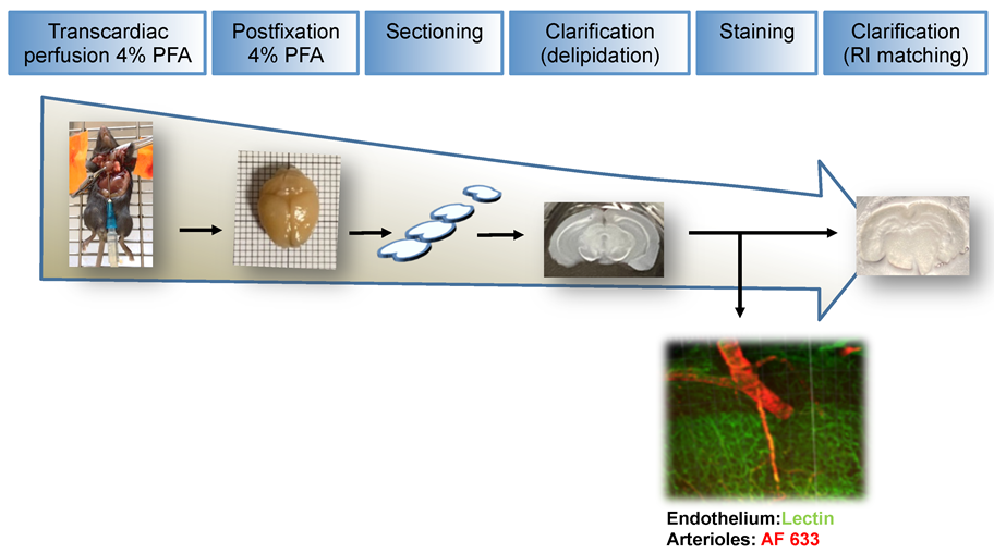
- Fixation: Samples were fixed using paraformaldehyde (PFA) after transcardiacally mice perfusion and dissection before post-fixation with PFA.
- 2.
- Sectioning: Here, m thick brain slices were sectioned using a vibratome.
- 3.
- Clearing: Sections were cleared using the CUBIC protocol.
- 4.
- Staining: Delipidated sections were stained with FITC-Lectin and an arteriole-specific dye Alexa Fluor 633 hydrazide.
- 5.
- Imaging: Here, m slices were analyzed using an advanced two-photon microscopy.
2.1. Fixation, Sectioning and Tissue Optical Clearing
2.2. Tissue Staining
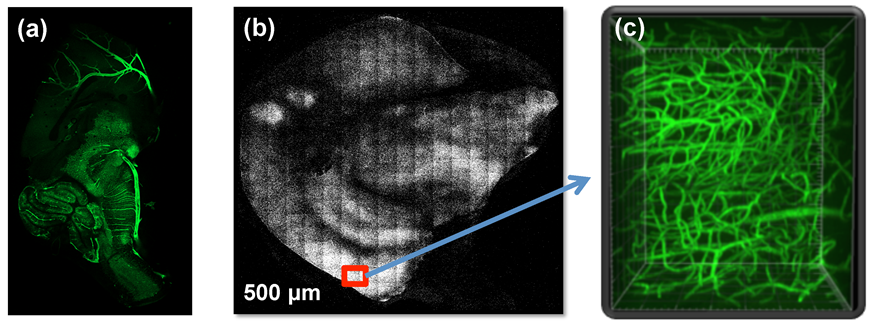
2.3. Two-Photon Excitation Microscopy
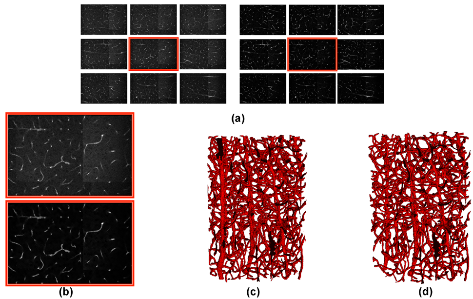
2.4. Image Analysis
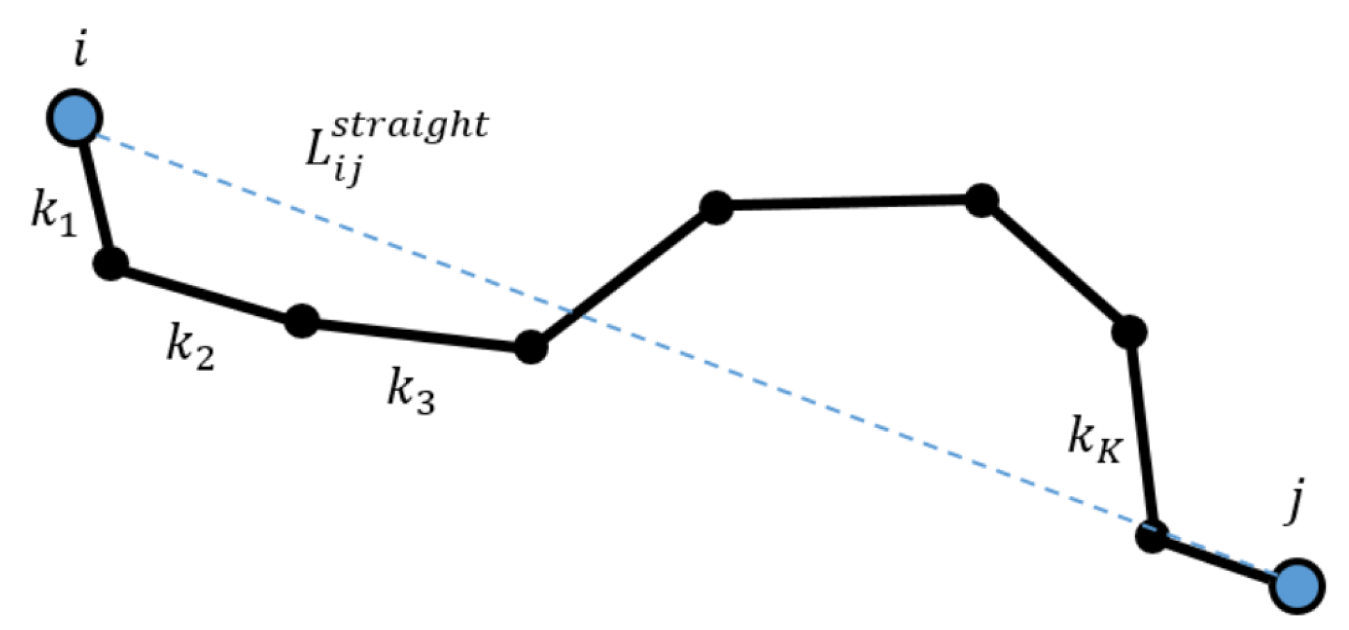
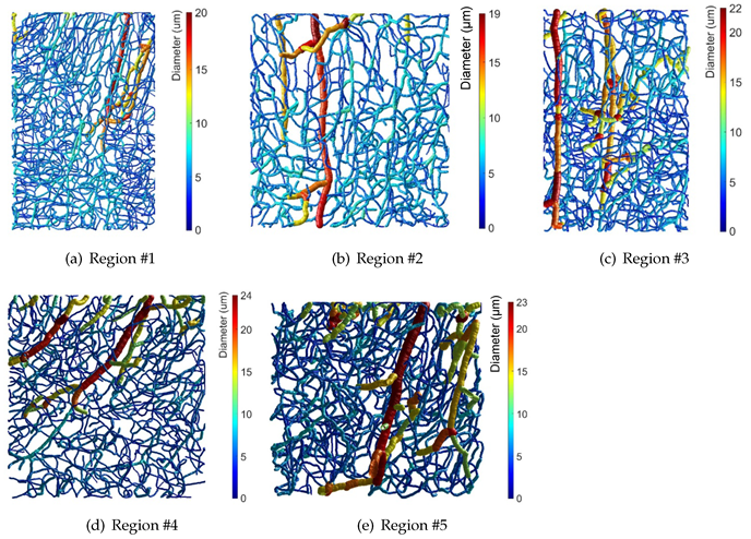
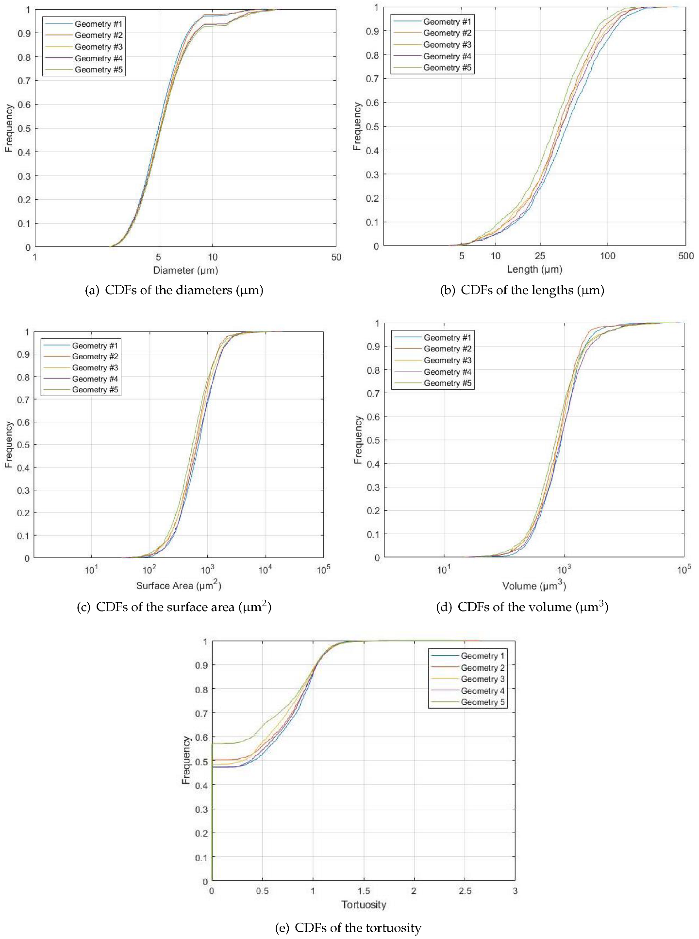
Vessel Measurements
2.5. One-Dimensional (1D) Modeling
2.5.1. Governing Equations
2.5.2. Boundary Conditions
- (a)
- Pressures were imposed at the inlet and outlets. With that, there was no need to know the flow direction in all in- and outflows respectively, as the flow direction in the segments adjusted to fulfill the pressure boundary conditions.
- (b)
- Boundary nodes (1 segment nodes) inside the geometries limits were assigned with a zero flow condition and with zero hematocrit. These nodes show the presence of broken vessels inside the geometry that could be produced during the segmentation. It is important to notice that these vessels have no physiological meaning but need to be treated.
- (c)
- Three different sets of pressure boundary conditions were assigned depending on the segment to which the boundary node was attached to: venule, arteriole or capillary:
- 1.
- At the arterial inflow, a pressure of 50 mmHg was given. The arterial pressure outflow was set to 40 or 45 mmHg depending on its nearness to the inflow. With that, the risk of a short circuit was eliminated.
- 2.
- At the venular outflows, a pressure of 10 mmHg was given.
- 3.
- In the capillary in/outflows, two cases were studied, following Lorthois and coworkers [5]:
- Case 1:
- Zero flow condition: Flow is set to zero in all the capillary outflows. In this case, the flow goes from the arterial inlet passing through the whole geometry until it reaches a venular outlet. As reported [5], this condition would underestimate the flow in the geometry as it isolates it from its virtual neighbors.
- Case 2:
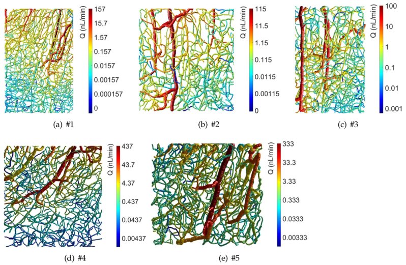
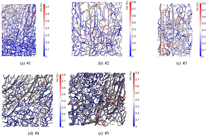
- Constant pressure condition: A constant capillary boundary pressure was calculated so that the net capillary flow (the sum of the flow in all the inlets and outlets) was zero; thus, everything that enters through the arterioles exits through the venules. In other words, this pressure was adjusted such that the total flow entering the arteriolar network was the same as the total flow entering the venular network. In this way, the net flux to all the boundary capillary segments was zero. As a consequence, the net flux leaving the studied brain region through capillaries to supply neighboring areas was exactly compensated by the net flux arriving from neighboring areas through capillaries. As shown in the literature, this condition forces the flux lines to be perpendicular to the ends of the computational domain, maximizing the exchanges of fluid with the neighboring region. For this reason, this condition overestimates the flow in the geometry as it maximizes the flow exchange between the region itself and its virtual neighbors. [64].
- (d)
3. Results
4. Discussion
5. Conclusions
Author Contributions
Funding
Institutional Review Board Statement
Data Availability Statement
Acknowledgments
Conflicts of Interest
References
- Boileau, E.; Nithiarasu, P.; Blanco, P.J.; Muller, L.O.; Eikeland Fossan, F.; Hellevik, L.R.; Donders, W.P.; Huberts, W.; Willemet, M.; Alastruey, J. A benchmark study of numerical schemes for one-dimensional arterial blood flow modelling. Int. J. Numer. Methods Biomed. Eng. 2015, 31, e02732. [Google Scholar] [CrossRef] [Green Version]
- Park, C.S.; Hartung, G.; Alaraj, A.; Du, X.; Charbel, F.T.; Linninger, A.A. Quantification of blood flow patterns in the cerebral arterial circulation of individual (human) subjects. Int. J. Numer. Methods Biomed. Eng. 2020, 36, e3288. [Google Scholar] [CrossRef] [PubMed]
- Cassot, F.; Lauwers, F.; Fouard, C.; Prohaska, S.; Lauwers-Cances, V. A novel three-dimensional computer-assisted method for a quantitative study of microvascular networks of the human cerebral cortex. Microcirculation 2006, 13, 1–18. [Google Scholar] [CrossRef] [PubMed]
- Lauwers, F.; Cassot, F.; Lauwers-Cances, V.; Puwanarajah, P.; Duvernoy, H. Morphometry of the human cerebral cortex microcirculation: General characteristics and space-related profiles. Neuroimage 2008, 39, 936–948. [Google Scholar] [CrossRef] [PubMed]
- Lorthois, S.; Cassot, F.; Lauwers, F. Simulation study of brain blood ow regulation by intra-cortical arterioles in an anatomically accurate large human vascular network: Part I: Methodology and baseline flow. NeuroImage 2011, 54, 1031–1042. [Google Scholar] [CrossRef] [Green Version]
- Lorthois, S.; Cassot, F.; Lauwers, F. Simulation study of brain blood flow regulation by intra-cortical arterioles in an anatomically accurate large human vascular net- work. Part II: Flow variations induced by global or localized modifcations of arteriolar diameters. NeuroImage 2011, 54, 2840–2853. [Google Scholar] [CrossRef] [Green Version]
- Schmid, F.; Reichold, J.; Weber, B.; Jenny, P. The impact of capillary dilation on the distribution of red blood cells in artificial networks. Am. J. Physiol.—Heart Circ. Physiol. 2015, 308, H733–H742. [Google Scholar] [CrossRef] [Green Version]
- Schmid, F.; Tsai, P.S.; Kleinfeld, D.; Jenny, P.; Weber, B. Depth-dependent flow and pressure characteristics in cortical microvascular networks. PLoS Comput. Biol. 2017, 13, e1005392. [Google Scholar] [CrossRef]
- Linninger, A.; Hartung, G.; Badr, S.; Morley, R. Mathematical synthesis of the cortical circulation for the whole mouse brain-part I. theory and image integration. Comput. Biol. Med. 2019, 110, 265–275. [Google Scholar] [CrossRef]
- Kidoguchi, K.T.; Mizobe, M.T.; Koyama, J.; Kondoh, T.; Kohmura, E.; Sakurai, T.; Yokono, K.; Umetani, K. In vivo X-ray angiography in the mouse brain using synchrotron radiation. Stroke 2006, 37, 1856–1861. [Google Scholar] [CrossRef]
- Fang, Q.; Sakadzić, S.; Ruvinskaya, L.; Devor, A.; Dale, A.M.; D, A.B. Oxygen Advection and Diffusion in a Three Dimensional Vascular Anatomical Network. Opt. Express. 2008, 16, 17530–17541. [Google Scholar] [CrossRef] [Green Version]
- Tsai, P.S.; Kaufhold, J.P.; Blinder, P.; Friedman, B.; Drew, P.J.; Karten, H.J.; Lyden, P.D.; Kleinfeld, D. Correlations of neuronal and microvascular densities in murine cortex revealed by direct counting and colocalization of nuclei and vessels. J. Neurosci. 2009, 29, 14553–14570. [Google Scholar] [CrossRef] [Green Version]
- Gould, I.G.; Linninger, A.A. Hematocrit Distribution and Tissue Oxygenation in Large Microcirculatory Networks. Microcirculation 2015, 12, 1–18. [Google Scholar] [CrossRef]
- Gould, I.G.; Tsai, P.; Kleinfeld, D.; Linninger, A. The capillary bed offers the largest hemodynamic resistance to the cortical blood supply. J. Cereb. Blood Flow Metab. 2017, 37, 52–68. [Google Scholar] [CrossRef] [Green Version]
- Gagnon, L.; Smith, A.F.; Boas, D.A.; Devor, A.; Secomb, T.W.; Sakadzić, S. Modeling of Cerebral Oxygen Transport Based on In vivo Microscopic Imaging of Microvascular Network Structure, Blood Flow, and Oxygenation. Front. Comput. Neurosci. 2016, 10, 82. [Google Scholar] [CrossRef] [Green Version]
- Hartung, G.; Badr, S.; Moeini, M.; Lesage, F.; Kleinfeld, D.; Alaraj, A.; Linninger, A. Voxelized simulation of cerebral oxygen perfusion elucidates hypoxia in aged mouse cortex. PLoS Comput. Biol. 2021, 17, 1008584. [Google Scholar] [CrossRef]
- Chen, Q.; Jiang, L.; Li, C.; Hu, D.; Bu, J.; Cai, D.; Du, J. Haemodynamics-driven developmental pruning of brain vasculature in zebrafish. PLoS Biol. 2012, 10, e1001374. [Google Scholar] [CrossRef] [Green Version]
- Blumers, A.L.; Yin, M.; Nakajima, H.; Hasegawa, Y.; Li, Z.; Karniadakis, G.E. Multiscale parareal algorithm for long-time mesoscopic simulations of microvascular blood flow in zebrafish. Comput. Mech. 2021, 68, 1131–1152. [Google Scholar] [CrossRef]
- Roustaei, M.; In Baek, K.; Wang, Z.; Cavallero, S.; Satta, S.; Lai, A.; O’Donnell, R.; Vedula, V.; Ding, Y.; Marsden, A.L.; et al. Computational simulations of the 4D micro-circulatory network in zebrafish tail amputation and regeneration. J. R. Soc. Interface 2022, 19, 29210898. [Google Scholar] [CrossRef]
- Anbazhakan, S.; Rios Coronado, P.E.; Sy-Quia, A.N.L.; Seow, A.; Hands, A.M.; Zhao, M.; Dong, M.L.; Pfaller, M.; Raftrey, B.C.; Cook, C.K.; et al. Blood flow modeling reveals improved collateral artery performance during the regenerative period in mammalian hearts. Nat. Cardiovasc. Res. 2022, 1, 775–790. [Google Scholar] [CrossRef]
- Ronellenfitsch, H.; Katifori, E. Global optimization, local adaptation, and the role of growth in distribution networks. Phys. Rev. Lett. 2016, 117, 138301. [Google Scholar] [CrossRef] [PubMed] [Green Version]
- Rocks, J.; Ronellenfitsch, H.; Liu, A.J.; Katifori, E. Limits of multifunctionality in tunable networks. Proc. Natl. Acad. Sci. USA 2019, 116, 2506–2511. [Google Scholar] [CrossRef] [PubMed] [Green Version]
- Sangiorgi, S.; De Benedictis, A.; Protasoni, M.; Manelli, A.; Reguzzoni, M.; Cividini, A.; Dell’Orbo, C.; Tomei, G.; Balbi, S. Early-stage microvascular alterations of a new model of controlled cortical traumatic brain injury: 3D morphological analysis using scanning electron microscopy and corrosion casting. J. Neurosurg. 2013, 118, 763–774. [Google Scholar] [CrossRef] [PubMed]
- Hartung, G.; Vesel, C.; Morley, R.; Alaraj, A.; Sled, J.; Kleinfeld, D.; Linninger, A. Simulations of blood as a suspension predicts a depth dependent hematocrit in the circulation throughout the cerebral cortex. PLoS Comput. Biol. 2018, 14, e1006549. [Google Scholar] [CrossRef]
- Schmid, F.; Barrett, M.J.P.; Obrist, D.; Weber, B.; Jenny, P. Red blood cells stabilize flow in brain microvascular networks. PLoS Comput. Biol. 2019, 15, e1007231. [Google Scholar] [CrossRef] [Green Version]
- Plouraboue, F.; Cloetens, P.; Fonta, C.; Steyer, A.; Lauwers, F.; Marc-Vergnes, J.P. X-ray high-resolution vascular network imaging. J. Microsc. 2004, 215, 139–148. [Google Scholar] [CrossRef]
- Heinzer, S.; Kuhn, G.; Krucker, T.; Ulmann-Schuler, E.M.A.; Stampanoni, M.; Gassmann, M.; Marti, H.H.; Muller, R.; Vogel, J. Novel three-dimensional analysis tool for vascular trees indicates complete micro-networks, not single capillaries, as the angiogenic endpoint in mice overexpressing human VEGF(165) in the brain. NeuroImage 2008, 39, 1549–1558. [Google Scholar] [CrossRef] [Green Version]
- Reichold, J.; Stampanoni, M.; Keller, L.; Buck, A.; Jenny, P.; Weber, B. Vascular graph model to simulate the cerebral blood flow in realistic vascular networks. J. Cereb. Blood Flow Metab. 2009, 29, 1429–1443. [Google Scholar] [CrossRef] [Green Version]
- Waelchli, T.; Bisschop, J.; Miettinen, A.; Ulmann-Schuler, A.; Hintermueller, C.; Meyer, E.P.; Krucker, T.; Waelchli, R.; Monnier, P.P.; Carmeliet, P.; et al. Hierarchical imaging and computational analysis of three-dimensional vascular network architecture in the entire postnatal and adult mouse brain. Nat. Protoc. 2021, 16, 4564–4610. [Google Scholar] [CrossRef]
- Reichold, J. Cerebral Blood Flow Modeling in Realistic Cortical Microvascular Networks. Ph.D. Thesis, Faculty of Science, ETH Zürich, Zürich, Switzerland, 2011. [Google Scholar]
- Demene, C.; Tiran, E.A.; Sieu, L.; Bergel, A.; Gennisson, J.L.; Pernot, M.; De Eux, T.; Cohen, I.; Tanter, M. 4D microvascular imaging based on ultrafast Doppler tomography. NeuroImage 2016, 127, 472–483. [Google Scholar] [CrossRef]
- Hlushchuk, R.; Haberthuer, D.; Soukup, P.; Barré, S.F.; Khoma, O.Z.; Schittny, J.; Jahromi, N.H.; Bouchet, A.; Engelhardt, B.; Djonov, V. Innovative high-resolution microCT imaging of animal brain vasculature. Brain Struct. Funct. 2020, 225, 2885–2895. [Google Scholar] [CrossRef]
- Ghavanati, S.; Yu, L.X.; Lerch, J.P.; Sled, J.G. A perfusion procedure for imaging of the muse cerebral vasculature by X-ray micro-CT. J. Neurosci. Methods 2014, 221, 70–77. [Google Scholar] [CrossRef] [Green Version]
- Chung, K.; Wallace, J.; Kim, S.Y.; Kalyanasundaram, S.; Andalman, A.S.; Davidson, T.J.; Mirzabekov, J.J.; Zalocusky, K.A.; Mattis, J.; Denisin, A.K.; et al. Structural and molecular interrogation of intact biological systems. Nature 2013, 497, 332–337. [Google Scholar] [CrossRef]
- Susaki, E.A.; Tainaka, K.; Perrin, D.; Kishino, F.; Tawara, T.; Watanabe, T.M.; Yokoyama, C.; Onoe, H.; Eguchi, M.; Yamaguchi, S.; et al. Whole-brain imaging with single-cell resolution using chemical cocktails and computational analysis. Cell 2014, 157, 726–739. [Google Scholar] [CrossRef] [Green Version]
- Dodt, H.U.; Leischner, U.; Schierloh, A.; Jahrling, N.; Mauch, C.P.; Deininger, K.; Deussing, J.M.; Eder, M.; Zieglgansberger, W.; Becker, K. Ultramicroscopy: Three-dimensional visualization of neuronal networks in the whole mouse brain. Nat. Methods 2007, 4, 331–336. [Google Scholar] [CrossRef] [PubMed]
- Ertuerk, A.; Becker, K.; Jaehrling, N.; Mauch, C.P.; Hojer, C.D.; Egen, G.J.; Hellal, F.; Bradke, F.; Sheng, M.; Dodt, H.U. Three-dimensional imaging of solvent-cleared organs using 3DISCO. Nat. Protoc. 2012, 7, 1983–1995. [Google Scholar] [CrossRef]
- Hama, H.; Kurokawa, H.; Kawano, H.; Ando, R.; Shimogori, T.; Noda, H.; Fukami, K.; Sakaue-Sawano, A.; Miyawaki, A. Scale: A chemical approach for fluorescence imaging and reconstruction of transparent mouse brain. Nat. Neurosci. 2011, 14, 1481–1488. [Google Scholar] [CrossRef]
- Ke, M.T.; Fujimoto, S.; Imai, T. SeeDB: A simple and morphology-preserving optical clearing agent for neuronal circuit reconstruction. Nat. Neurosci. 2013, 16, 1154–1161. [Google Scholar] [CrossRef]
- Renier, N.; Wu, Z.; Simon, D.J.; Yang, J.; Ariel, P.; Tessier-Lavigne, M. iDISCO: A simple, rapid method to immunolabel large tissue samples for volume imaging. Cell 2014, 159, 896–910. [Google Scholar] [CrossRef] [Green Version]
- Li, Y.; Xu, J.; Wan, P.; Yu, T.; Zhu, D. Optimization of GFP fluorescence preservation by a modified uDISCO clearing protocol. Front. Neuroanat. 2021, 12, 67. [Google Scholar] [CrossRef] [PubMed]
- Chung, K.; Deisseroth, K. CLARITY for mapping the nervous system. Nat. Methods 2013, 10, 508–513. [Google Scholar] [CrossRef] [PubMed]
- Tomer, R.; Ye, L.; Hsueh, B.; Deisseroth, K. Advanced CLARITY for rapid and high-resolution imaging of intact tissues. Nat. Protoc. 2014, 9, 1682–1697. [Google Scholar] [CrossRef] [Green Version]
- Spence, R.D.; Kurtha, F.; Itoh, N.; Mongerson, C.R.L.; Wailes, S.H.; Peng, M.S.; MacKenzie-Graham, A.J. Bringing CLARITY to gray matter atrophy. NeuroImage 2014, 101, 625–632. [Google Scholar] [CrossRef] [Green Version]
- Zheng, H.; Rinaman, L. Simplified CLARITY for visualizing immunofluorescence labeling in the developing rat brain. Brain Struct. Funct. 2016, 2375–2383, 221. [Google Scholar] [CrossRef] [Green Version]
- Poplawsky, A.J.; Fukuda, M.; Bok-man, K.; Hwan-Kim, J.; Suh, M.; Kim, S.G. Dominance of layer-specific microvessel dilation in contrast-enhanced high-resolution fMRI: Comparison between hemodynamic spread and vascular architecture with CLARITY. NeuroImage 2019, 197, 657–667. [Google Scholar] [CrossRef]
- Martínez-Lorenzana, G.; Gamal-Eltrabily, M.; Tello-García, I.A.; Martínez-Torres, A.; Becerra-González, M.; González-Hernández, A.; Condés-Lara, M. CLARITY with neuronal tracing and immunofluorescence to study the somatosensory system in rats. J. Neurosci. Methods 2020, 350, 109048. [Google Scholar] [CrossRef]
- Ren, Z.; Wu, Y.; Wang, Z.; Hu, Y.; Lu, J.; Liu, J.; Chen, Y.; Yao, M. CUBIC-plus: An optimized method for rapid tissue clearing and decolorization. Biochem. Biophys. Res. Commun. 2021, 568, 116–123. [Google Scholar] [CrossRef]
- Tainaka, K.; Kubota, S.I.; Suyama, T.Q.; Susaki, E.A.; Perrin, D.; Ukai-Tadenuma, M.; Ukai, H.; Ueda, H.R. Whole-body imaging with single-cell resolution by tissue decolorization. Cell 2014, 159, 911–924. [Google Scholar] [CrossRef] [Green Version]
- Susaki, E.A.; Tainaka, K.; Perrin, D.; Yukinaga, H.; Kuno, A.; Ueda, H.R. Advanced CUBIC protocols for whole-brain and whole-body clearing and imaging. Nat. Protoc. 2015, 10, 1709–1727. [Google Scholar] [CrossRef] [Green Version]
- Pinheiro, T.; Mayor, I.; Edwards, S.; Joven, A.; Kantzer, C.G.; Kirkham, M.; Simon, A. CUBIC-f: An optimized clearing method for cell tracing and evaluation of neurite density in the salamander brain. J. Neurosci. Methods 2021, 348, 109002. [Google Scholar] [CrossRef]
- Hasegawa, S.; Susaki, E.A.; Tanaka, T.; Komaba, H.; Wada, T.; Fukagawa, M.R.; Ueda, H.; Nangaku, M. Comprehensive three-dimensional analysis (CUBIC-kidney) visualizes abnormal renal sympathetic nerves after ischemia/reperfusion injury. Kidney Int. 2019, 96, 129–138. [Google Scholar] [CrossRef]
- Murakami, T.C.; Mano, T.; Saikawa, S.; Horiguchi, S.A.; Shigeta, D.; Baba, K.; Sekiya, H.; Shimizu, Y.; Tanaka, K.F.; Kiyonari, H.; et al. A three-dimensional single-cell-resolution whole-brain atlas using CUBIC-X expansion microscopy and tissue clearing. Nat. Neurosci. 2018, 21, 625–637. [Google Scholar] [CrossRef] [PubMed]
- Matsumoto, K.; Mitani, T.T.; Horiguchi, S.A.; Kaneshiro, J.; Murakami, T.C.; Mano, T.; Fujishima, H.; Konno, A.; Watanabe, T.M.; Hirai, H.; et al. Advanced CUBIC tissue clearing for whole-organ cell profiling. Nature Protocols 2021, 14, 3506–3537. [Google Scholar] [CrossRef] [PubMed]
- Karc, R.; Neumann, F.; Neumann, M.; Schreiner, W. Staged growth of optimized arterial model trees. Ann. Biomed. Eng. 2000, 28, 495–511. [Google Scholar] [CrossRef] [PubMed]
- Karch, R.; Neumann, F.; Podesser, B.K.; Neumann, M.; Szawlowski, P.; Schreiner, W. Fractal properties of perfusion heterogeneity in optimized arterial trees: A model study. J. Gen. Physiol. 2003, 122, 307–322. [Google Scholar] [CrossRef] [Green Version]
- Schreiner, W.; Karch, R.; Neumann, M.; Neumann, F.; Roedler, S.M.; Heinze, G. Heterogeneous perfusion is a consequence of uniform shear stress in optimized arterial tree models. J. Theor. Biol. 2003, 3, 285–301. [Google Scholar] [CrossRef] [Green Version]
- Sakadzic, S.; Roussakis, E.; Yaseen, M.A.; Mandeville, E.T.; Srinivasan, V.J.; Arai, K.; Ruvinskaya, S.; Devor, A.; Lo, E.H.; Vinogradov, S.A.; et al. Two-photon high-resolution measurement of partial pressure of oxygen in cerebral vasculature and tissue. Nat. Methods 2010, 7, 755–759. [Google Scholar] [CrossRef] [Green Version]
- Blinder, P.; Shih, A.Y.; Rafie, C.; Kleinfeld, D. Topological basis for the robust distribution of blood to rodent neocortex. Proc. Natl. Acad. Sci. USA 2010, 107, 12670–12675. [Google Scholar] [CrossRef] [Green Version]
- Keller, A.L.; Schuz, A.; Logothetis, N.K.; Weber, B. Vascularization of cytochrome oxidase-rich blobs in the primary visual cortex of squirrel and macaque monkeys. J. Neurosci. 2011, 31, 1246–1253. [Google Scholar] [CrossRef] [Green Version]
- Kasischke, K.A.; Lambert, E.M.; Panepento, B.; Sun, A.; Gelbard, H.A.; Burgess, R.W.; Foster, T.H.; Nedergaard, M. Two-photon NADH imaging exposes boundaries of oxygen diffusion in cortical vascular supply regions. J. Cereb. Blood Flow Metab. 2011, 31, 68–81. [Google Scholar] [CrossRef]
- Sherwin, S.J.; Franke, V.; Peiró, J.; Parker, K. One-dimensional modelling of a vascular network in space-time variables. J. Eng. Math. 2003, 47, 217–250. [Google Scholar] [CrossRef]
- Boas, D.A.; Jones, S.R.; Devor, A.; Huppert, T.J.; Dale, A.M. A vascular anatomical network model of the spatio-temporal response to brain activation. NeuroImage 2008, 40, 1116–1129. [Google Scholar] [CrossRef] [PubMed] [Green Version]
- Lorthois, S.; Cassot, F. Fractal analysis of vascular networks: Insights from morphogenesis. J. Theor. Biol. 2010, 262, 614–633. [Google Scholar] [CrossRef] [PubMed] [Green Version]
- Peyrounette, M.; Davit, Y.; Quintard, M.; Lorthois, S. Multiscale modelling of blood ow in cerebral microcirculation: Details at capillary scale control accuracy at the level of the cortex. PLoS ONE 2018, 13, e0189474. [Google Scholar] [CrossRef] [PubMed]
- Linninger, A.A.; Gould, I.G.; Marinnan, T.; Hsu, C.Y.; Chojecki, M.; Alaraj, A. Cerebral Microcirculation and Oxygen Tension in the Human Secondary Cortex. Ann. Biomed. Eng. 2013, 41, 2264–2284. [Google Scholar] [CrossRef] [PubMed]
- Hsu, C.Y.; Schneller, B.; Alaraj, A.; Flannery, M.; Zhou, X.J.; Linninger, A. Automatic recognition of subject-specifc cerebrovascular trees. Magn. Reson. Med. 2016, 77, 398–410. [Google Scholar] [CrossRef] [Green Version]
- Hsu, C.Y.; Ghaffari, M.; Alaraj, A.; Flannery, M.; Zhou, X.J.; Linninger, A. Gap-free segmentation of vascular networks with automatic image processing pipeline. Comput. Biol. Med. 2017, 82, 29–39. [Google Scholar] [CrossRef] [Green Version]
- Buades, A.; Coll, B.; Morel, J.M. A Non-Local Algorithm for Image Denoising. IEEE Comput. Soc. Conf. Comput. Vis. Pattern Recognit. 2005, 2, 60–65. [Google Scholar]
- Hasinoff, S.W. Photon, Poisson Noise. In Computer Vision; Ikeuchi, K., Ed.; Springer: Boston, MA, USA, 2014. [Google Scholar]
- Zana, F.; Klein, J.C. Segmentation of vessel-like patterns using mathematical morphology and curvature evaluation. IEEE Trans. Image Process. 2001, 10, 1010–1019. [Google Scholar]
- Bradley, D.; Roth, G. Adapting Thresholding Using the Integral Image. J. Graph. Tools 2007, 12, 13–21. [Google Scholar] [CrossRef]
- Soille, P. Morphological Image Analysis: Principles and Applications; Springer: Berlin/Heidelberg, Germany, 1999. [Google Scholar]
- Lee, T.C.; Kashyap, R.L.; Chu, C.N. Building skeleton models via 3-D medial surface/axis thinning algorithms. Comput. Vis. Graph. Image Process. 1994, 56, 462–478. [Google Scholar] [CrossRef]
- Kerschnitzki, M.; Kollmannsberger, P.; Burghammer, M.; Duda, G.N.; Weinkamer, R.; Wagermaier, W.; Fratzl, P. Architecture of the osteocyte network correlates with bone material quality. J. Bone Miner. Res. 2013, 28, 1837–1845. [Google Scholar] [CrossRef]
- Pries, A.R.; Secomb, T.W. Blood Flow in Microvascular Networks. In Microcirculation; Elsevier: Amsterdam, The Netherlands, 2008; pp. 3–36. [Google Scholar]
- Schmid, F. Cerebral Blood Flow Modeling with Discrete Red Blood Cell Tracking Analyzing Microvascular Networks and Their Perfusion. Ph.D. Thesis, Faculty of Science. ETH Zurich, Zürich, Switzerland, 2017. [Google Scholar]
- Pries, A.R.; Secomb, T.W.; Gebner, T.; Sperandio, M.B.; Gross, J.F.; Gaehtgens, P. Resistance to Blood Flow in Microvessels In Vivo. Circ. Res. 1994, 75, 904–915. [Google Scholar] [CrossRef] [Green Version]
- Shapiro, H.M.; Stromberg, D.D.; Lee, D.R.; Wiederhielm, C.A. Dynamic pressures in the pill arterial microcirculation. Am. J. Physiol.-Leg. Content 1971, 221, 279–283. [Google Scholar] [CrossRef]
- Bullit, E.; Gerig, G.; Pizer, S.M.; Lin, W.; Aylward, S.R. Measuring tortuosity of the intracerebral vasculature from MRA images. IEEE Trans. Med. Imaging 2003, 22, 1163–1171. [Google Scholar] [CrossRef] [Green Version]
- Su, S.W.; Catherall, M.; Payne, S. The influence of network structure on the transport of blood in the human cerebral microvasculature. Microcirculation 2012, 19, 175–187. [Google Scholar] [CrossRef]
- Lee, R.M. Morphology of cerebral arteries. Pharmacol. Ther. 1995, 66, 149–173. [Google Scholar] [CrossRef]
- Olufsen, M.S. A structured tree outflow condition for blood flow in larger systemic arteries. Am. J. Physiol. 1999, 276, H257–H268. [Google Scholar] [CrossRef]
- Olufsen, M.S.; Peskins, C.S.; Kim, W.Y.; Pedersen, E.M.; Nadim, A.; Larsen, J. Numerical simulation and experimental validation of blood flow in arteries with structured tree outflow conditions. Ann. Biomed. Eng. 2000, 28, 1281–1299. [Google Scholar] [CrossRef]
- Malvè, M.; Chandra, S.; García, A.; Mena, A.; Martínez, M.A.; Finol, E.A.; Doblaré, M. Impedance-based outflow boundary conditions for human carotid haemodynamics. Comput. Methods Biomech. Biomed. Eng. 2014, 17, 1248–1260. [Google Scholar] [CrossRef]
- El-Bouri, W.K.; Payne, S.J. Multi-scale homogenization of blood ow in 3-dimensional human cerebral microvascular networks. J. Theor. Biol. 2015, 380, 40–47. [Google Scholar] [CrossRef] [PubMed]
- Bui, A.V.; Manasseh, R.; Liffman, K.; Šutalo, I.D. Development of optimized vascular fractal tree models using level set distance function. Med. Eng. Phys. 2010, 32, 790–794. [Google Scholar] [CrossRef] [PubMed]


| Region | Nodes | Boundary Nodes | Segments | Dimensions (m) |
|---|---|---|---|---|
| 1250 | 210 | 1561 | ||
| 751 | 136 | 932 | ||
| 968 | 134 | 1265 | ||
| 948 | 198 | 1164 | ||
| 999 | 72 | 1292 |
Publisher’s Note: MDPI stays neutral with regard to jurisdictional claims in published maps and institutional affiliations. |
© 2022 by the authors. Licensee MDPI, Basel, Switzerland. This article is an open access article distributed under the terms and conditions of the Creative Commons Attribution (CC BY) license (https://creativecommons.org/licenses/by/4.0/).
Share and Cite
Mañosas, S.; Sanz, A.; Ederra, C.; Urbiola, A.; Rojas-de-Miguel, E.; Ostiz, A.; Cortés-Domínguez, I.; Ramírez, N.; Ortíz-de-Solórzano, C.; Villanueva, A.; et al. An Image-Based Framework for the Analysis of the Murine Microvasculature: From Tissue Clarification to Computational Hemodynamics. Mathematics 2022, 10, 4593. https://doi.org/10.3390/math10234593
Mañosas S, Sanz A, Ederra C, Urbiola A, Rojas-de-Miguel E, Ostiz A, Cortés-Domínguez I, Ramírez N, Ortíz-de-Solórzano C, Villanueva A, et al. An Image-Based Framework for the Analysis of the Murine Microvasculature: From Tissue Clarification to Computational Hemodynamics. Mathematics. 2022; 10(23):4593. https://doi.org/10.3390/math10234593
Chicago/Turabian StyleMañosas, Santiago, Aritz Sanz, Cristina Ederra, Ainhoa Urbiola, Elvira Rojas-de-Miguel, Ainhoa Ostiz, Iván Cortés-Domínguez, Natalia Ramírez, Carlos Ortíz-de-Solórzano, Arantxa Villanueva, and et al. 2022. "An Image-Based Framework for the Analysis of the Murine Microvasculature: From Tissue Clarification to Computational Hemodynamics" Mathematics 10, no. 23: 4593. https://doi.org/10.3390/math10234593