Quantitative Criteria for the Degree of Pathological Remodeling of the Aortic Duct

Abstract

Analysis of the properties of the aorta was carried out by numerous researchers using several parameters. However, the general laws of change in the dynamic geometry of the aortic flow channel in connection with the hydrodynamics of the swirling blood flow have not been studied properly. Therefore, at present, attempts to correct various diseases are carried out based on the location of the aneurysm, and not in accordance with the general patterns of changes in the dynamic geometry of the entire aortic channel. For a proper understanding of the aortic flow channel remodeling mechanisms, it is necessary to determine the quantitative parameters that formalize the geometry of this channel. The geometric shape of the aorta primarily depends on the hydrodynamics of the flow inside the aortic flow channel, which is the only source of force impact on its walls. The main result of the present study was that we obtained the new quantitative parameters that characterize the normal aorta and the degree of its shape deviations caused by pathological changes of the aortic duct. These parameters were calculated based on the software processing of the three-dimensional aortic reconstruction in normal conditions and in the case of differently localized aortic aneurysm.

1. Introduction

Any perturbations in the blood stream, which is a biologically active fluid flowing in a channel with biologically active walls, inevitably lead to the activation of the body’s defense systems and/or damage to the walls of the flow channel. Therefore, the main hypothesis is that the blood flow in the central parts of the circulatory system (heart and great vessels) is carried out without the formation of separation and stagnant zones, that is, it is a potential flow. In such a flow, by definition, any types of interaction are minimized both in the flow core and on the walls of the flow channel.

The cellular composition of the walls [1,2], their biomechanical properties [1], the distribution of velocities and shear stresses [3,4], and metabolism [5,6] were studied. Many model studies of the aorta have been carried out [7]. However, by present days there are no proper quantitative criterions that allow one to formalize the degree of aortic duct pathological remodeling. In the present study these parameters have been obtained by considering analytical solutions for the velocity vector of swirling blood flow in the heart and great vessels.

2. Materials and Methods

In previously published works [8,9,10], it has been shown that the dynamic geometry of the heart and great vessels corresponds with a high degree of accuracy to the direction of streamlines of swirling flows described by exact solutions of the Navier-Stokes and continuity equations for a class of self-organizing tornado-like flows of a viscous fluid. These solutions were obtained in 1986 by G.I. Kiknadze and Yu.K. Krasnov [11] and are generally expressed by relation (1).

$$\{\begin{array}{c}{u}_r=C_0\left(t\right)r+\frac{C_1}{r}\\ u_z=-2C_0\left(t\right)z+C_2\left(t\right)\\ u_{\phi }\left(r,t\right)=\frac{1}{r}\ast \left(A_1+A_2\Gamma \left(1+\frac{C_1}{2\upsilon }, \alpha \left(0\right)\ast r^2\right)\right),\end{array}$$

(1)

Here $C_0\left(t\right)$ and $C_2\left(t\right)$ are time-dependent functions, $A_1$, $A_2$, and $C_1$ are constants, and $\alpha \left(t\right)$ is a function that has the following form:

$$\alpha \left(t\right)=\frac{e^{-2{{\displaystyle \int }}_0^t{C}_0\left({\tau }_1\right)d{\tau }_1}}{B_1-A{{\displaystyle \int }}_0^t{e}^{-2{{\displaystyle \int }}_0^{\tau }{C}_0\left({\tau }_2\right)d{\tau }_2}d{\tau }_1}$$

Here $B_1$—is the arbitrary constant.

In the steady state, the swirling flow under consideration can be described by the relations for the Burgers vortex [12]:

$$\{\begin{array}{c}{u}_r=-C_0\ast r\\ u_z=2C_0\ast z\\ u_{\phi }=\frac{{\Gamma }_0}{2\pi r}\ast \left(1-e^{-\frac{C_0^2\ast r}{2\nu }}\right)\end{array}$$

(2.1)

However, it is known that the blood flow is roughly unsteady and occurs in a pulsating regime. Previously, it has been shown [13,14] that the geometry of the flow channel during the entire cardiac cycle corresponds to the direction of the streamlines described by these solutions. Therefore, we used these solutions as quasi-stationary, if only $C_0\left(t\right)$ and ${\Gamma }_0\left(t\right)$ depend on time. In this case, relation (2.1) may be transformed as follows:

$$\{\begin{array}{c}{u}_r=-C_0\left(t\right)\ast r\\ u_z=2C_0\left(t\right)\ast z\\ u_{\phi }=\frac{{\Gamma }_0\left(t\right)}{2\pi r}\ast \left(1-e^{-\frac{C_0^2\left(t\right)\ast r}{2\nu }}\right)\end{array}$$

(2.2)

Here, only the azimuthal velocity component depends on the viscosity; therefore, the modulus of this component decreases with the evolution of the flow.

The geometry of the flow channel must correspond to the direction of the streamlines of the swirling flow inside. Expression (2.2) includes two functions of time—$C_0\left(t\right)$ and ${\Gamma }_0\left(t\right)$. To use these solutions as quasi-stationary in a non-stationary pulsating flow, the cardiac cycle was considered as a sequence of discrete states, in each of which the flow is described by relations (2.1). In this case, the instantaneous values of $C_0\left(t\right)$ and ${\Gamma }_0\left(t\right)$ are described by the measured geometric characteristics of the flow channel.

The instantaneous position of the streamlines of the considered flow in the longitudinal-radial projection is described by the following relation:

$$z{r}^2=\beta \left(t\right)$$

(3)

$\beta \left(t\right)$—a time-dependent function, the instantaneous value of which is determined by the choice of values $C_0$ and ${\Gamma }_0$ at a given time.

Streamlines in a fixed position of the flow channel of the heart and aorta in the axial-radial projection are described by the following expression:

$$\phi =\frac{{\Gamma }_0}{2\pi C_0}\ast \left(\frac{1}{r}+\sqrt{\frac{\pi C_0}{2\upsilon }}\ast \underset{0}{\overset{\sqrt{\frac{C_0}{2\upsilon }}r}{{\displaystyle \int }}}{e}^{-t^2}dt-\frac{1}{r}\ast e^{-\frac{C_0{r}^2}{2\upsilon }}\right)+{\phi }_0$$

(4)

As has been shown already, the aorta retains the shape of a converging canal throughout the entire cardiac cycle [13]. According to our assumptions, the pulse oscillations of the aortic wall are much less than the geometric transformations that occur in the process of remodeling. Therefore, the aortic flow channel was normally considered as a tube with almost constant geometric characteristics. As a result, fluctuations in the values of the characteristics $C_0$ and ${\Gamma }_0$ were considered negligible.

Since the streamlines are an evolution of the hyperbolic helix (4), continuous flow along such streamlines is possible only in a channel that has the form of a lower order hyperbolic right-handed helix (with fewer turns per aortic length). To approximate the shape of the aortic flow channel, a flat hyperbolic spiral of the following form was used:

$$r={\left(\frac{a}{\phi }\right)}^{power}+bias$$

Here $\left(r, \varphi \right)$ are the radial and longitudinal coordinates, and $\left(a, power, bias\right)$ are the parameters by which the approximation is carried out.

As a result, the obtained quantitative characteristics of the shape of the aorta are composed of two components, which are the values taken by the constants $C_0$ and ${\Gamma }_0$ and the parameters describing the helical properties of the aortic flow channel.

Let us consider 2 sections of the aortic flow channel outlying at a distance $z_1$ and $z_2$ respectively from the plane of the aortic valve. The corresponding aortic radiuses on these sections are $r_1$ and $r_2$. For $z_1<z_2$ it follows that $r_1>r_2$ due to the convergence of the flow channel. Since the specific spatial location of the point of origin of the cylindrical coordinate system in which the parameters of the aortic flow channel were calculated is unclear, a fictitious point of origin was introduced into consideration, which is located at a distance z0 from the plane of the aortic valve inside the cavity of the left ventricle. This point can change its position during the entire cardiac cycle, however, within the framework of this work, it was assumed to be immobile. It can be considered as the point of origin of the swirling blood flow. Then relation (3) for the sections under consideration can be written as follows:

$$\left(z_0+z_1\right)\ast r_1^2=\left(z_0+z_2\right)\ast r_2^2\iff z_0=\frac{z_2{r}_2^2-z_1{r}_1^2}{r_1^2-r_2^2}$$

(5)

From (2.2) it can be derived that the contribution of the azimuthal component in the total swirling flow velocity vector decreases with the distance from the origin point. Thus, if a certain section of the aortic flow channel $S_1$ is closer to the point of origin than the section $S_2$, the corresponding value of the modulus of the azimuth component can be expressed as follows: $u_{\varphi ,1}>u_{\varphi ,2}$. Accordingly, the minimum value of $\left|u_{\varphi }\right|$ occurs near the end of the aorta. For simplicity it can be stated as $\left|u_{\varphi }\right|=0$. Then the total velocity vector through the section $S_2$ at the end of the aorta will be written as follows:

$$u_2=\sqrt{u_z^2+u_r^2}=C_0\sqrt{4{\left(z_0+z_2\right)}^2+r_2^2}\iff C_0=\frac{u_2}{\sqrt{4{\left(z_0+z_2\right)}^2+r_2^2}}$$

(6)

Considering the section $S_1$, the derived expression for the linear velocity of the swirling flow through this section can be written as follows:

$$\begin{array}{c}{u}_1=\sqrt{u_z^2+u_r^2+u_{\phi }^2}\iff u_{\phi }^2=u_1^2-u_z^2-u_r^2\iff {\left(\frac{{\Gamma }_0}{2\pi r}\ast \left(1-e^{-\frac{C_0^2\ast r_1}{2\nu }}\right)\right)}^2\\ =u_1^2-4C_0^2{\left(z_0+z_1\right)}^2-C_0^2{r}_1^2\end{array}$$

Expanding the brackets and simplifying the expression above, we get:

$${\Gamma }_0=\frac{\sqrt{4\pi r_1^2{u}_1^2-4\pi r_1^2{C}_0^2\left(4{\left(z_0+z_1\right)}^2+r_1^2\right)}}{\left(1-e^{-\frac{C_0^2\ast r_1}{2\nu }}\right)}$$

(7)

For the correct reconstruction of a parametric spatial curve approximating the shape of the aortic flow channel, it is necessary to reconstruct the central line of the aorta first.

The central line is a spatial curve drawn between two planes cutting through an extended cavity in such a way that the distance from this line to the boundaries of the cavity is the maximum.

To construct the central line, 2 planes were used that cut the aortic flow channel perpendicular to the direction of the swirling blood flow. For all studied aortas, one of these planes is the plane that includes the aortic valve. The algorithm for choosing another plane depends on the type of aorta. For a relatively healthy aorta, the second plane should coincide with the section of the aorta in a bifurcation zone; for an aorta with a pathological disorder of the vascular bed, the plane was chosen approximately at the level of 2/3 of the aorta length, counting from the aortic valve. This is due to a large distortion of the geometry of the aortic flow channel in the abdominal region, which is associated with serious errors in the reconstruction of the required central line. Then, points were fixed on the selected planes in the central region of the cutting planes (one for each plane). These points (labeled as $p_1$ and $p_2$) were used to construct the required center line.

To determine the central line, it is necessary to determine the trajectory $C=C\left(s\right)$ connecting the selected points $p_1$ and $p_2$. This trajectory should ensure the minimization of the value of the following functional:

$$I_{centerline}\left(C\right)={{\displaystyle \int }}_{C^{-1}\left(p_1\right)}^{C^{-1}\left(p_2\right)}F\left(C\left(s\right)\right)ds$$

(8)

In the written expression, $F\left(x\right)$ is a certain scalar field, the value of which at points lying closer to the center of the cavity is less than at points far from the center. The simplest example is a function whose value at a point is inversely proportional to the distance from this point to the boundary of the cavity. Such a function can be represented by the following relation:

$$DT\left(x\right)=\underset{y\in d\Omega }{min}\left(\left|x,y\right|\right)$$

(9)

In this relation, $\left|\left(x,y\right)\right|$ is the Euclidean distance from the point x to the point y, $d\Omega$ is the boundary of the cavity $\Omega$, corresponding to the radius of the channel at this point. Choosing the scalar field $F\left(x\right)=D{T}^{-1}\left(x\right)$ defined by expression (8), the central lines will need to be located on the medial axis of the given cavity $\Omega$. The medial axis of the cavity is defined as the set of ball centers inscribed in a given cavity, where the size of the inscribed ball will be the maximum only if it in turn is not inscribed in another such ball. The construction of such a medial axis and the central line associated with it is carried out using the Voronoi diagram [15]. In the three-dimensional case, the Voronoi diagram is a surface composed of convex polygons whose vertices are the centers of the maximum inscribed balls.

The construction of the Voronoi diagram was performed by Delaunay triangulation [16], which was accompanied by the removal of polygons that partially fell out of the given cavity. This method allowed us to reformulate the problem described by expression (6) in the form of an eikonal equation, a non-linear partial differential equation:

$$\left|\nabla T\left(x\right)=F\left(x\right)\right|$$

(10)

The boundary condition for the written equation is $T\left(p_1\right)=0$. Such an equation can be solved using the fast sweep method. As soon as the solution of equation (8) was obtained for the entire Voronoi diagram, the backpropagation method was used to construct a trajectory from point $p_1$ to point $p_2$ in the direction of the maximum decrease in the value of the scalar field (i.e., in the direction of the medial axis of the cavity).

Central lines have been constructed using The Vascular Modelling Toolkit (vmtk).

All required data engineering and math computations has been done using standard python packages—pandas, numpy, scipy, scikit-learn and vmtk.

3. Results

3.1. Computation of $C_0$ and ${\Gamma }_0$

Eighteen aortic conditions were studied in 14 patients, of which 4 had normal aortas, 6 had lesions located in the proximal regions, and 4 had lesions localized in the distal regions. Three-dimensional reconstructions of the aortas were obtained using MSCT.

Each reconstruction is a surface in STL format. The surfaces presented in this format are a set of conjugated triangles with indication of the normal to them. The following algorithm was used to calculate the $C_0$ and ${\Gamma }_0$ values for these reconstructions:

1. The initial matrix with the coordinates of the triangles that make up the surface of the aortic duct was presented as a matrix A with dimensions [num_rows, num_features]. Here num_rows is the total number of triangles that make up the surface, and num_features is the number of points representing each such triangle (num_features = 9 for 3D space).

2. The computed matrix A was projected onto a plane by the PCA method (there was a decrease in the dimension from 9 to 2). Next, the length of the 2d-projection of the aortic flow channel was measured, and on the distance from the beginning of the aorta by 10% and 90% of the entire length of the aorta, the aortic radius was measured. Thus, two pairs of values $\left(z_1,r_1\right)$ and $\left(z_2,r_2\right)$ were obtained, which are important for $C_0$ and ${\Gamma }_0$ computation according to expressions (5) and (6).

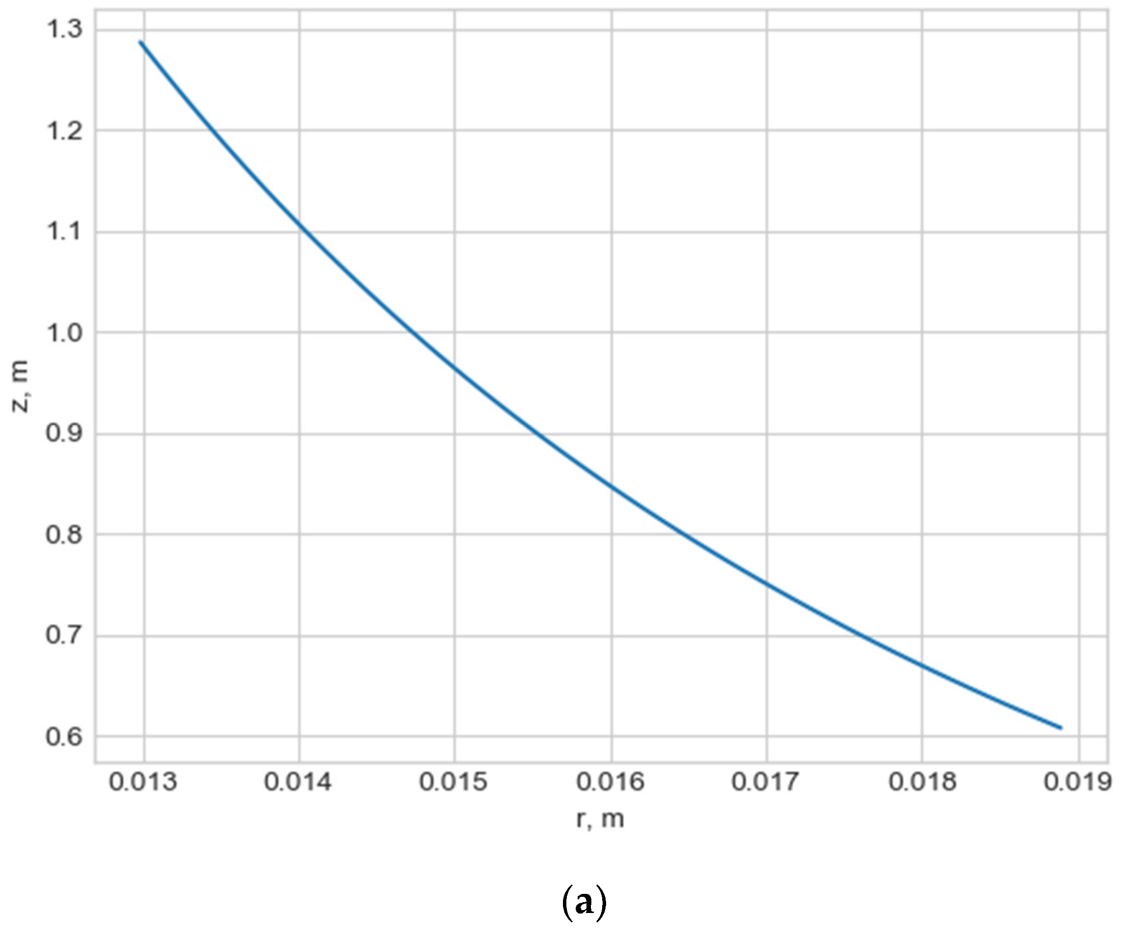
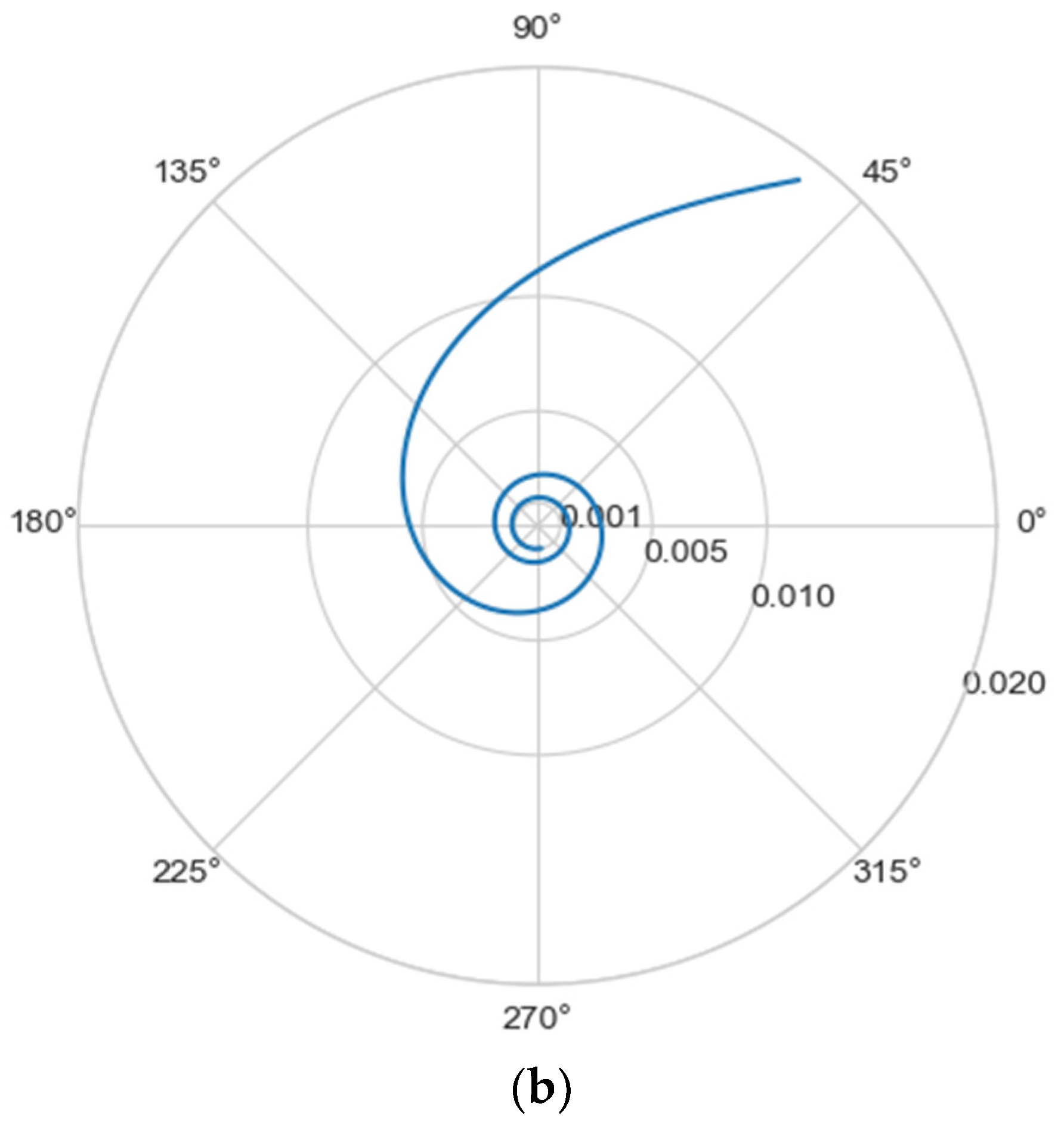
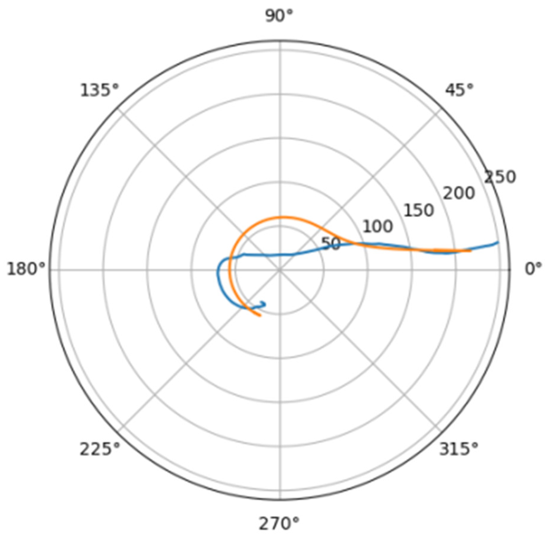
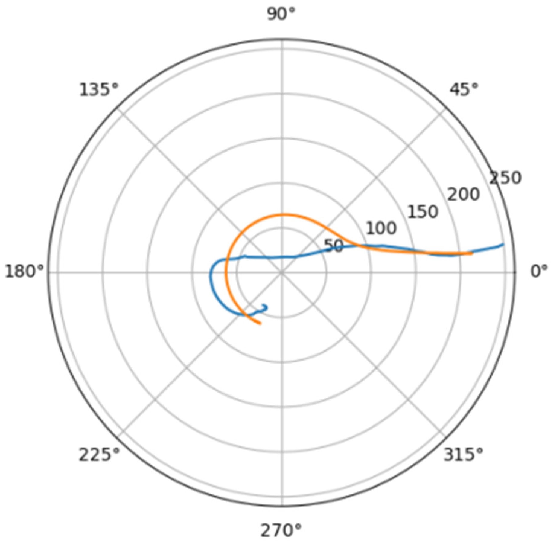
Normally, for patients without obvious aortic pathology, the streamlines can be plotted as follows (Figure 1a,b).

Figure 1b shows a plot of $C_0$ and ${\Gamma }_0$ values depending on the location of aortic pathology.

Table 1. Values of constants $C_0$ and ${\Gamma }_0$ for the studied aortas, ‘loc’—localization of aortic lesion (down—distal aneurysm, up—proximal aneurysm, norm—no pathology).

Name	${\mathit{C}}_0$ (s−1)	${\mathbf{\Gamma }}_0$ (m2/s)	loc
lar_s	0.301	0.046	up
hom_a	0.357	0.058	up
are_d	0.537	0.073	down
ino_d	0.407	0.070	down
mir_s	0.460	0.037	norm
lar_d	0.307	0.048	up
she_a	0.243	0.071	down
mal_a	0.135	0.076	down
zag_a	0.368	0.041	norm
mir_d	0.427	0.037	norm
are_s	0.378	0.068	down
pav_a	0.218	0.071	down
bor_a	0.545	0.089	down
gor_d	0.314	0.041	norm
poz_a	0.255	0.044	norm
bar_a	0.564	0.039	up
ino_s	0.396	0.072	down
bru_a	0.484	0.052	up

shows the corresponding values of the parameters $C_0$ and ${\Gamma }_0$.

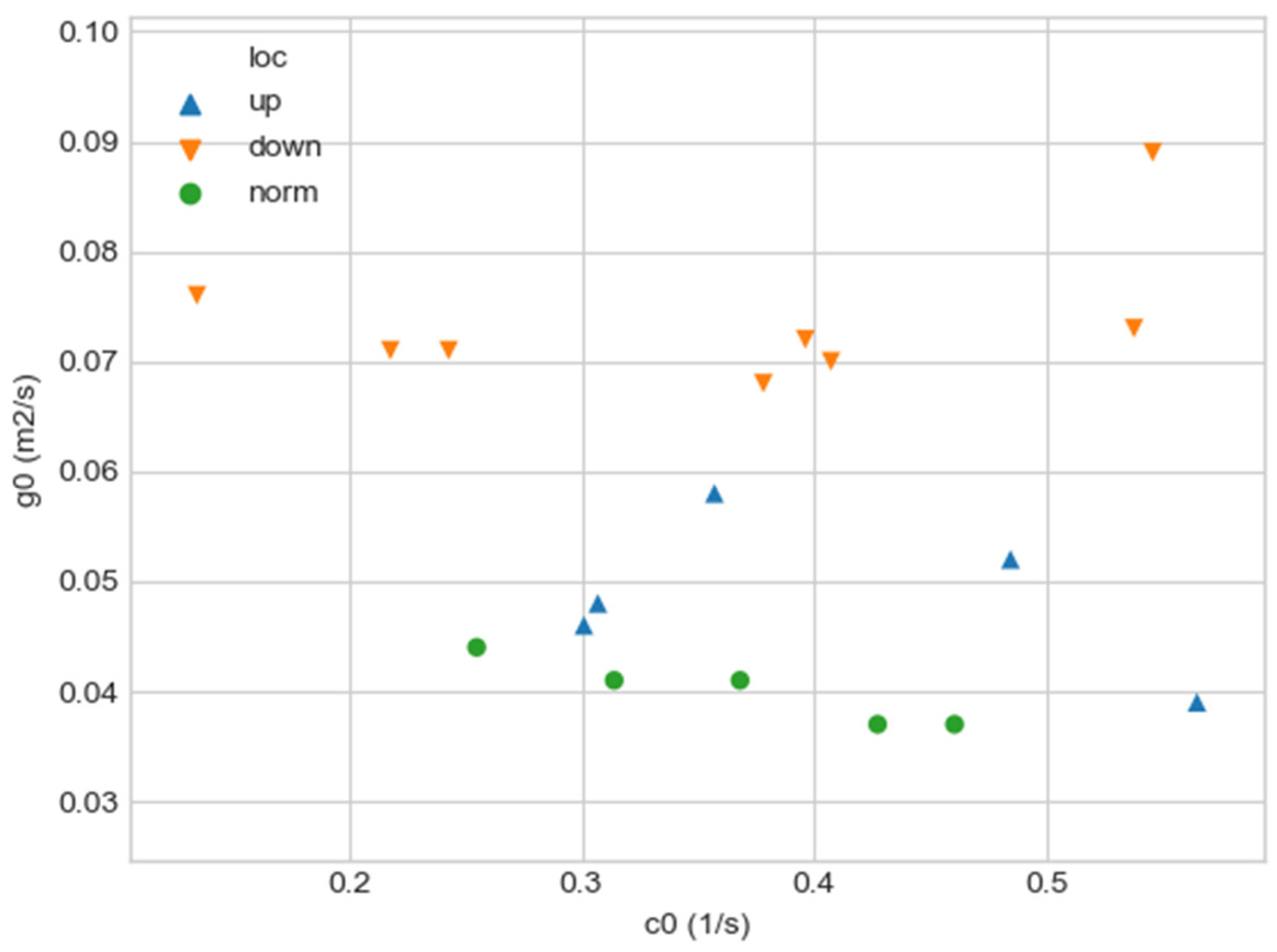
As can be seen in Figure 2, a pair of $C_0$ and ${\Gamma }_0$ values can serve as a quantitative criterion for identifying aortic pathology. All three considered cases (pathology in the descending aorta, pathology in the ascending aorta and the norm) are linearly separable.

In the case of a pathological disturbance of the vascular bed in the descending section, the value of the circulation ${\Gamma }_0$ of the swirling flow increases significantly. At the same time, a $C_0$ raising can be observed followed by the increase in the transverse gradients of the blood flow velocity. Fluctuations of $C_0$ and ${\Gamma }_0$ values may reflect the action of compensatory and regulatory mechanisms of the cardiovascular system. However, the actions of these mechanisms are inevitably associated with excessive energy consumption to maintain the flow structure and can also lead to an increased force impact on the aortic wall.

In the case of pathology in the ascending region, one can observe a slight increase in the ${\Gamma }_0$ value and a relatively small (compared with the pathology of the descending region) increase in $C_0$ value.

However, the parameters $C_0$ and ${\Gamma }_0$ do not unequivocally allow the establishment of the fact of pathological remodeling of the aortic duct. In Figure 1a,b, the dots representing aortas with distal damage lie very close to the dots corresponding to the normal aorta.

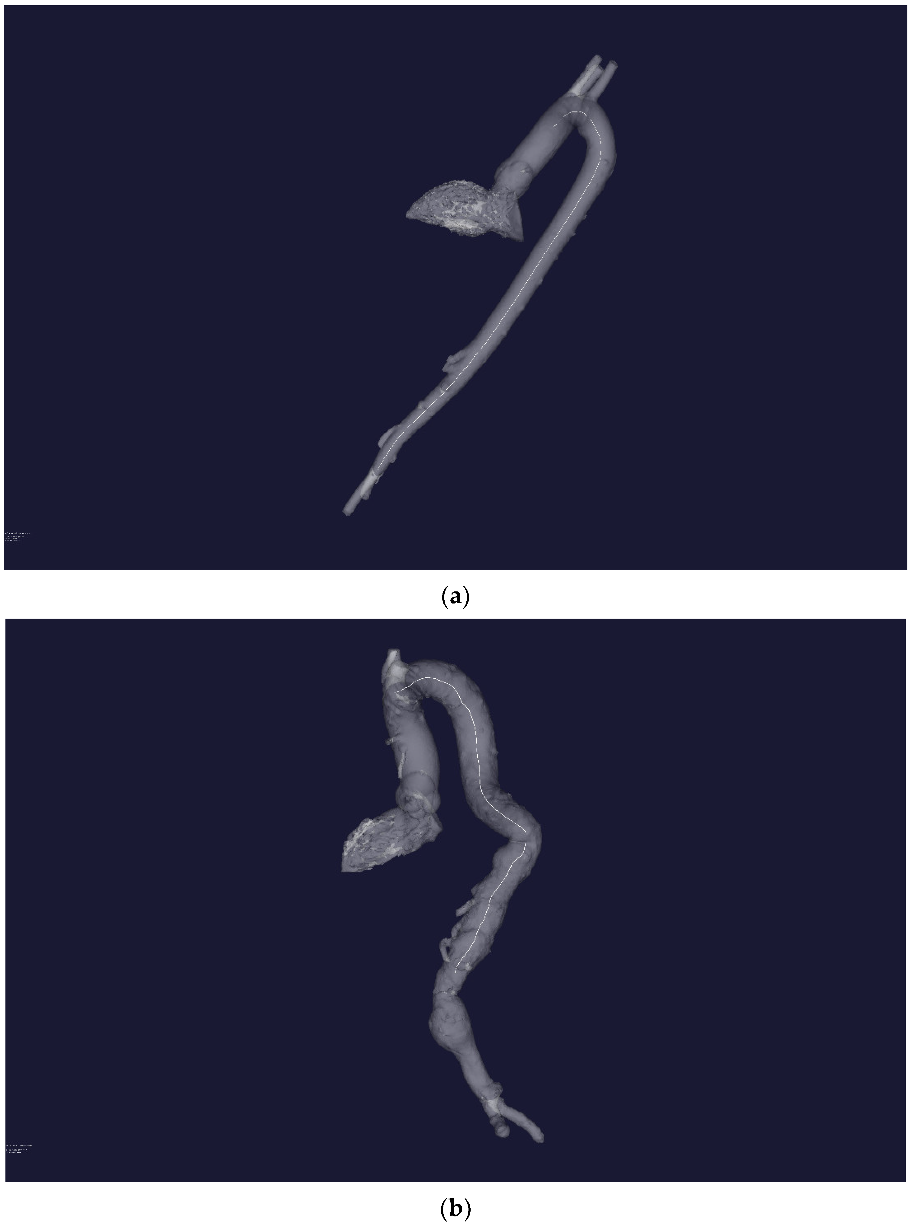
3.2. Approximation of the Aorta Flow Channel by a Parametric Spiral

Figure 3a,b show the result of plotting the central line for an aorta with no obvious pathological disorders and an aorta with pathology, respectively.

Each center line is a matrix with dimensions [num_points, 3], where num_points is the number of points in the center line, and 3 is the number of spatial dimensions in the Cartesian coordinate system. The resulting lines must be approximated by some spiral curves to obtain the characteristic parameters. The search for spirals was carried out in the class of hyperbolic spirals described by the following relation in the polar coordinate system:

$$r={\left(\frac{a}{\phi }\right)}^{power}+bias$$

(11)

In relation (11), the unknown parameters are $\left(a, power, bias\right)$.

The hyperbolic class of spirals was chosen since the streamlines of the swirling blood flow in the aorta in the radial-axial projection are described by a hyperbolic spiral, and the similarity principle indicates that the flow channel, in which the flow evolves without the formation of separation and stagnant zones, must have similar geometry.

For each central line, an approximating spiral was constructed in accordance with the following algorithm:

• The original [num_points, 3] centerline was projected onto a plane using the PCA method to obtain a [num_points, 2] matrix, where 2 is the (x, y) coordinates. The resulting projection is labeled centerline_proj.
• The coordinates of the resulting line centerline_proj were converted to the polar coordinate system $\left(r, \phi \right)$ using the following expressions:

  $$\begin{array}{c}r=\sqrt{x^2+y^2}\\ \phi =atan2\left(y, x\right)\end{array}$$

Here $atan2\left(y, x\right)$—2-argument arctangent used to translate Cartesian coordinates into polar coordinates. This arctangent can be stated as follows:

$$atan2\left(y, x\right)=\{\begin{array}{c}2arctan\left(\frac{y}{\sqrt{x^2+y^2}+x}\right), if x>0 and y\ne 0,\\ \pi , if x<0 and y=0,\\ undefined, if x=0 and y=0\end{array}$$

Using the least squares method, the parameters $\left(a, power, bias\right)$ from expression (11) were selected in such a way that the polar representation of the centerline_proj line is most accurately described by the parametric hyperbolic spiral (11).

The obtained parameters of the approximating spiral $\left(a, power, bias\right)$, the coefficient of determination $R^2$, and the standard deviation (mae) of the real line centerline_proj from the approximating spiral were entered in the resulting table.

Based on the calculated five parameters $\left(a, power, bias, R^2, mae\right)$. 2 synthetic parameters were calculated by the PCA method (feature_1, feature_2). These parameters store all the necessary information about the quantitative differences in the parameters $\left(a, power, bias, R^2, mae\right)$ for the normal aorta and in the presence of a pathological change in the vascular bed and allow visual interpretation of these differences.

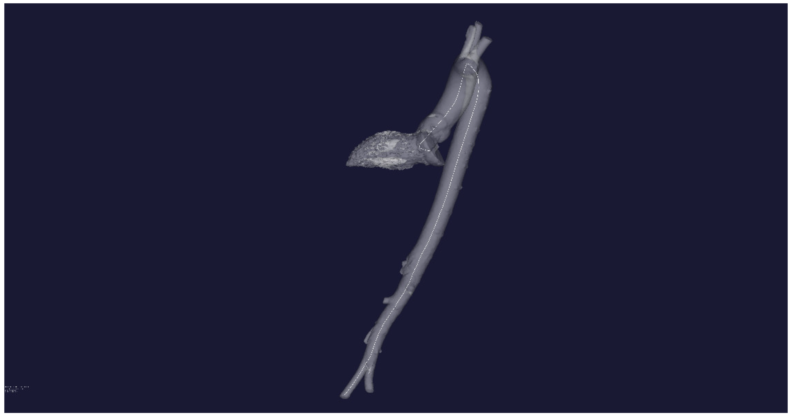
The application of the formulated algorithm for one central line looks like this:

The plotting of the initial three-dimensional central line centerline (white line) is performed in Figure 4.

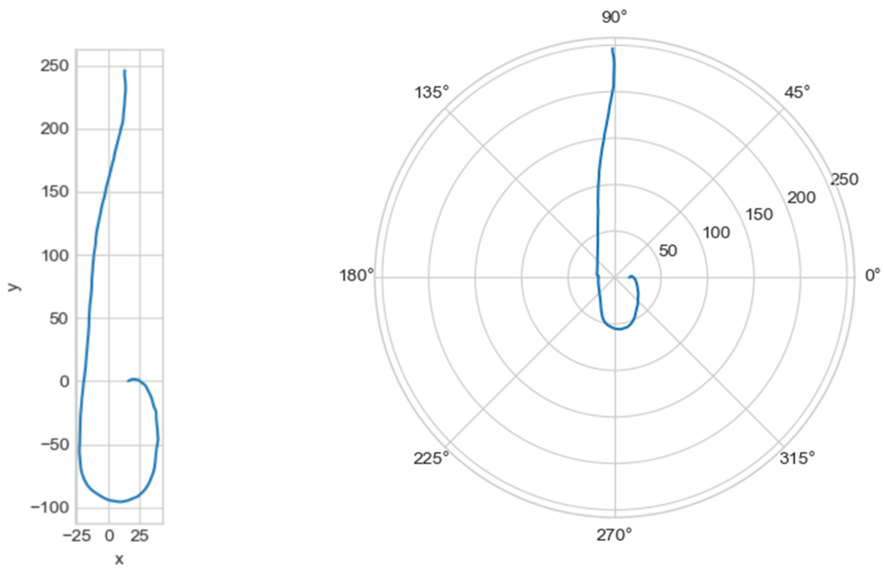
The graph of the line centerline_proj was plotted, with the projection of the central line onto the plane in Cartesian and polar coordinate systems (Figure 5).

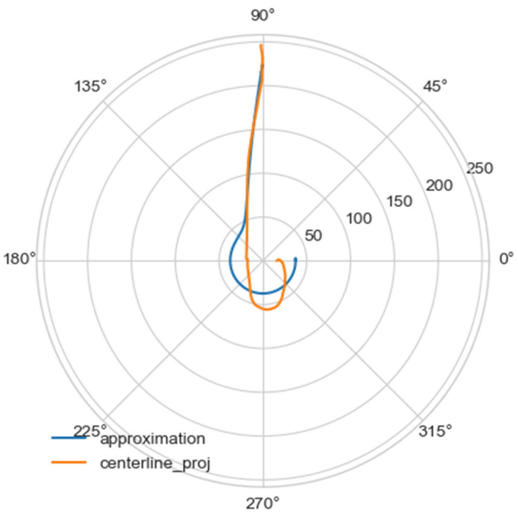
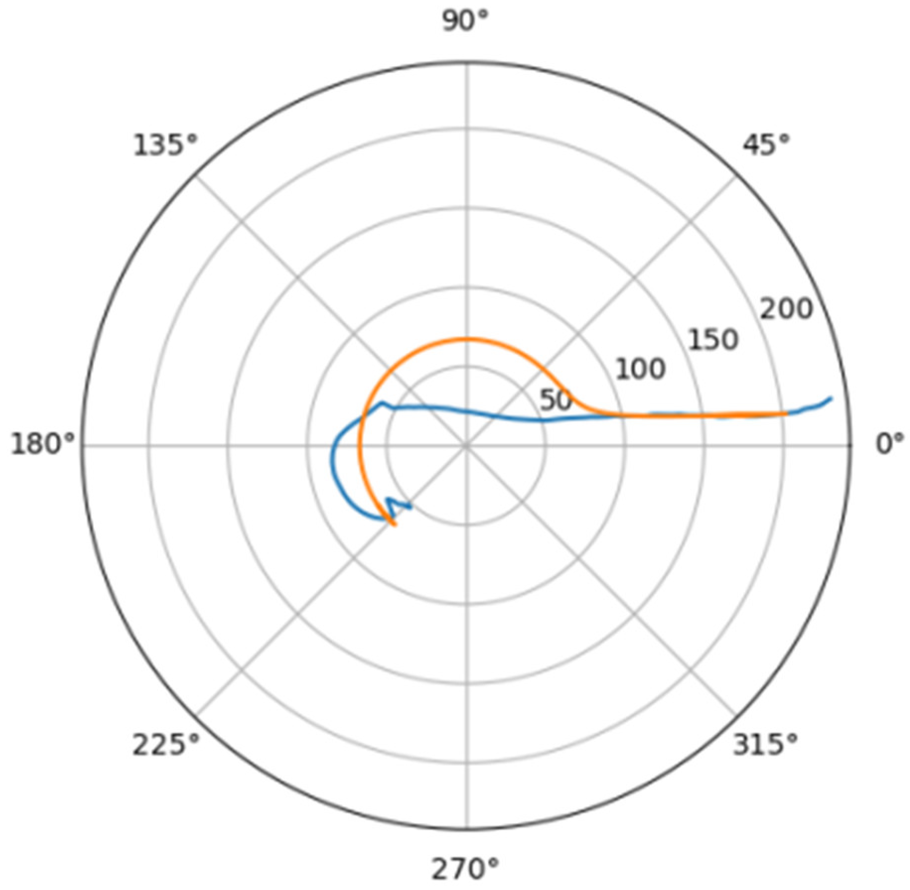
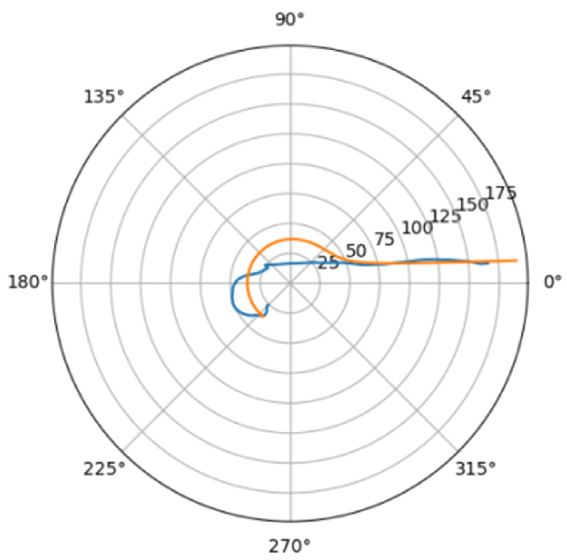
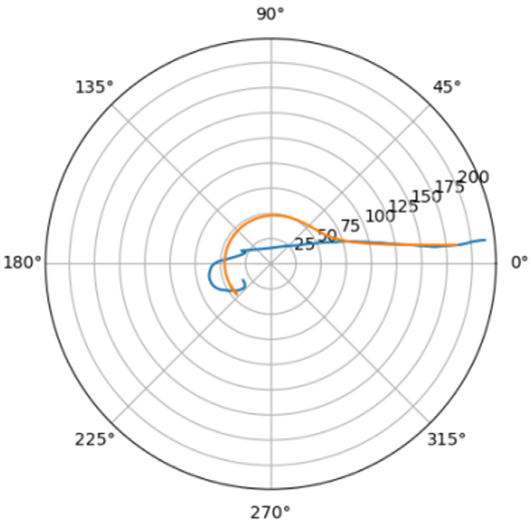
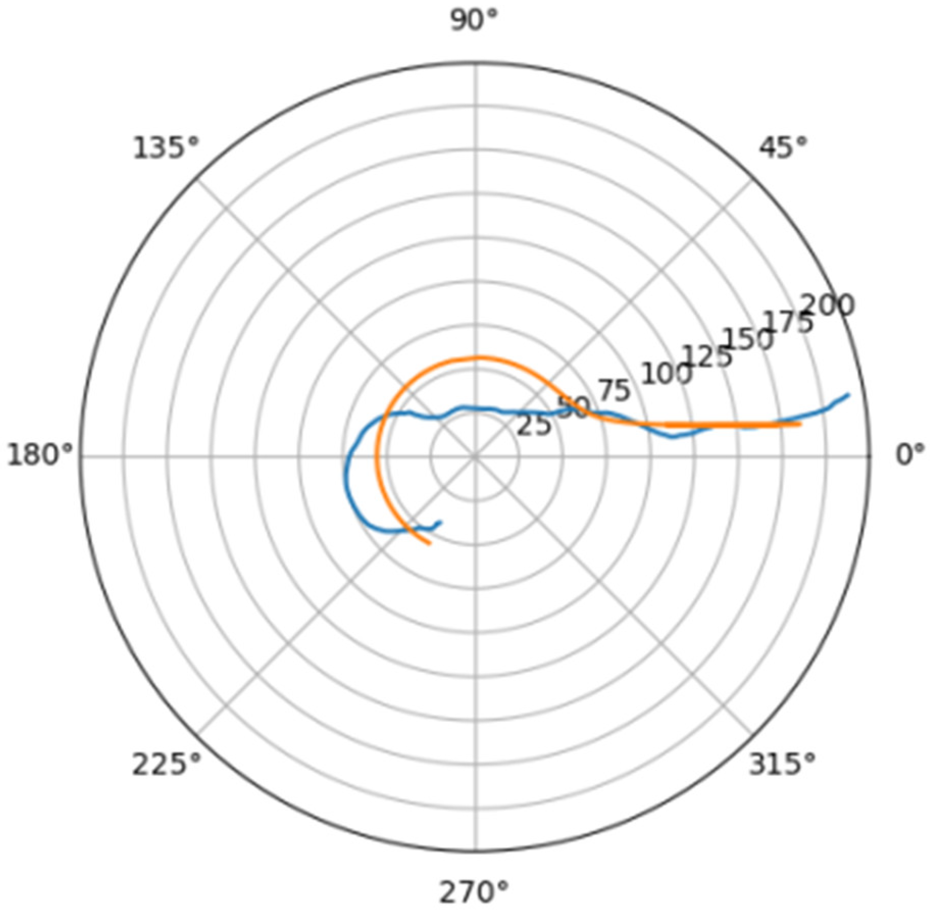
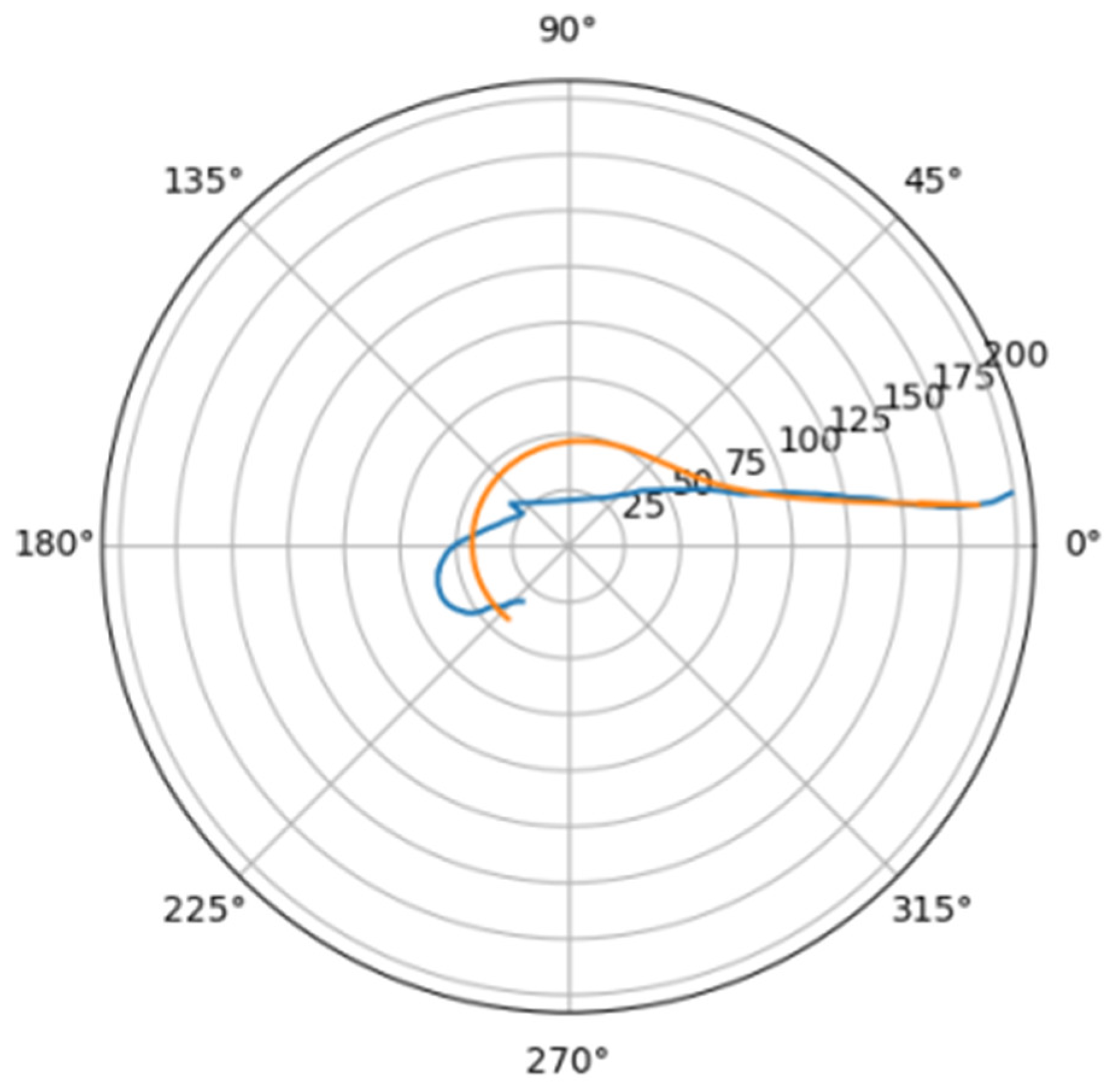
Using the least squares method, the parameters of the approximating spiral were calculated. In Figure 6, the original curve and its approximation are plotted in the polar coordinate system.

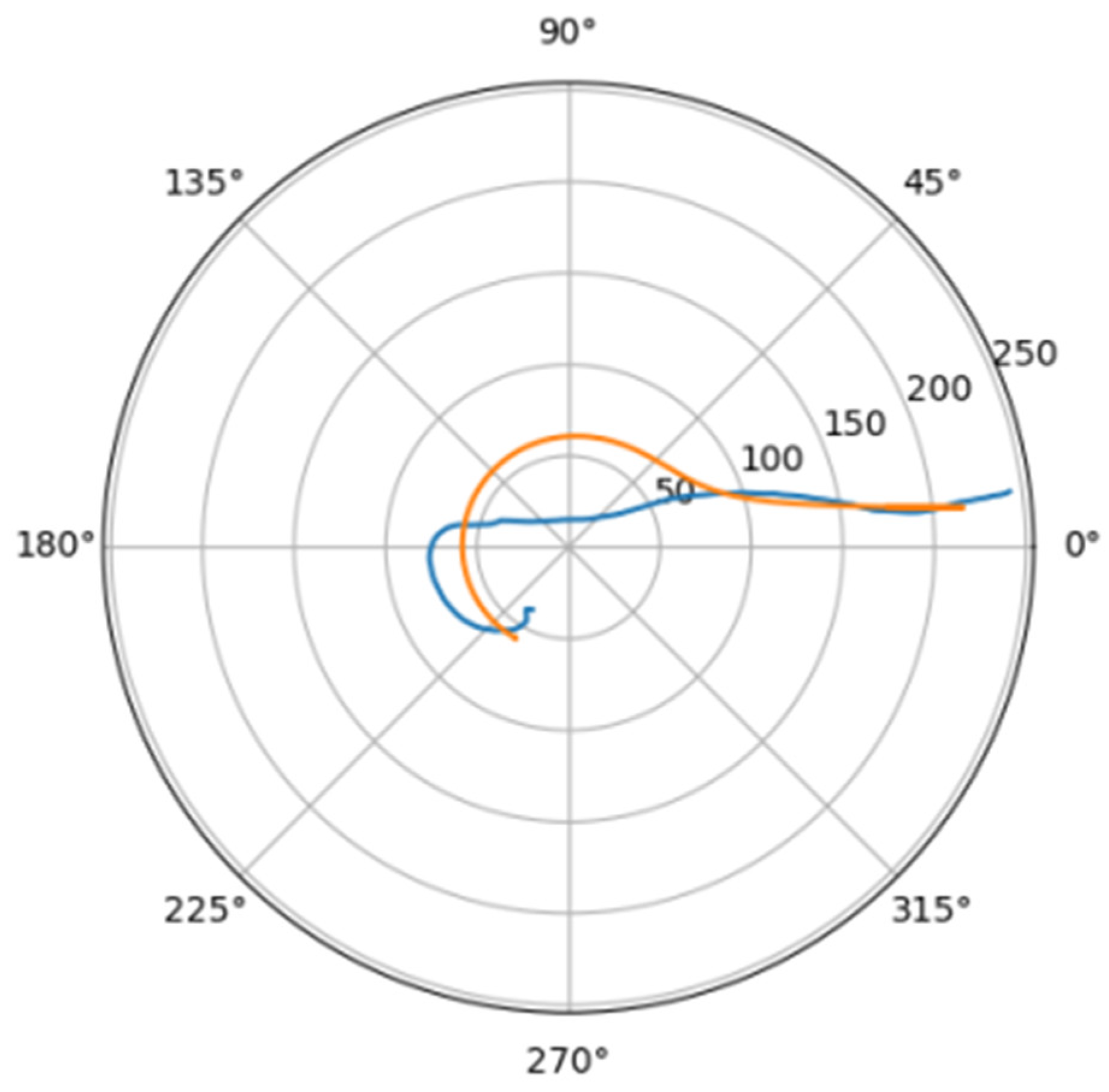
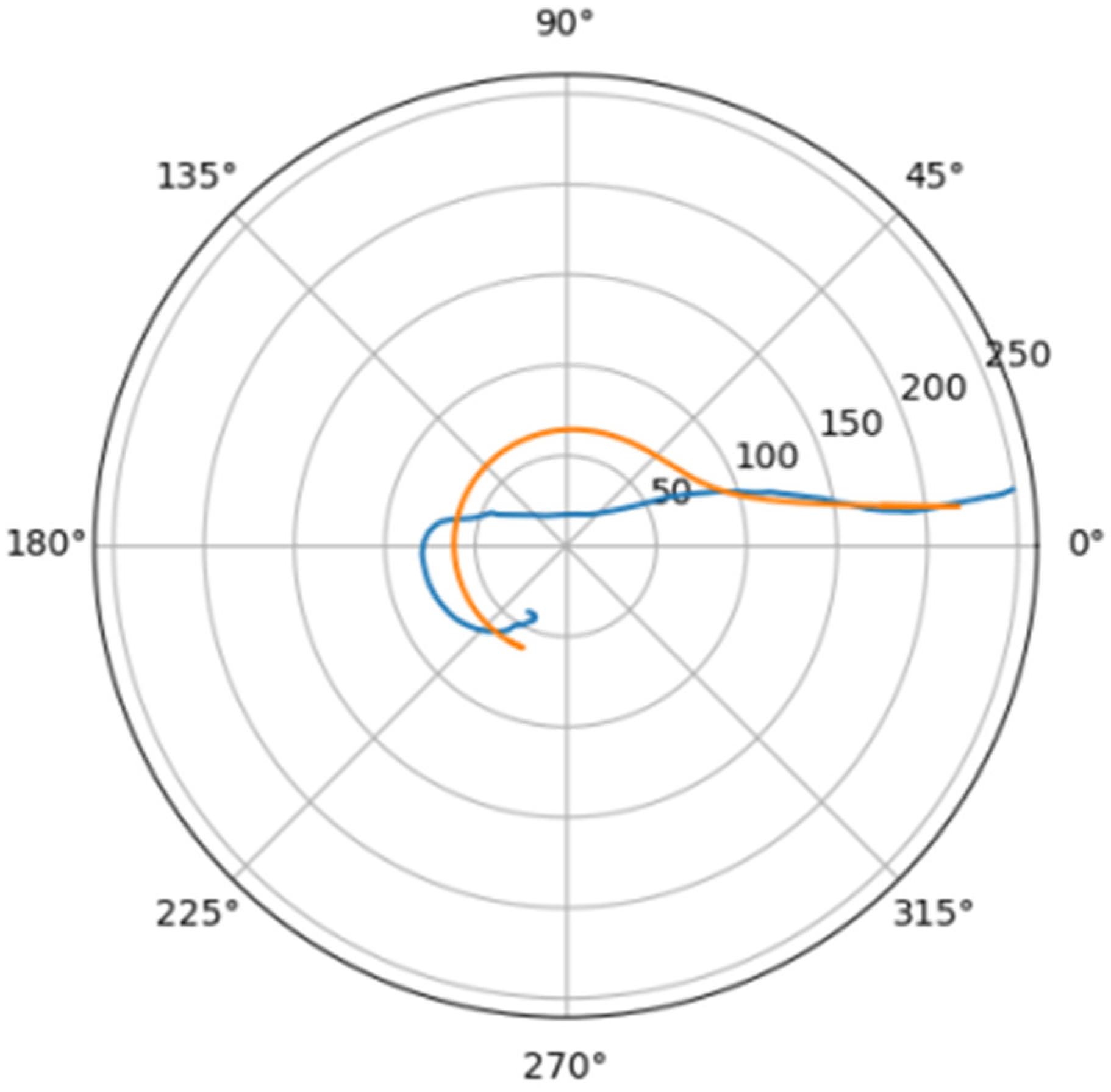
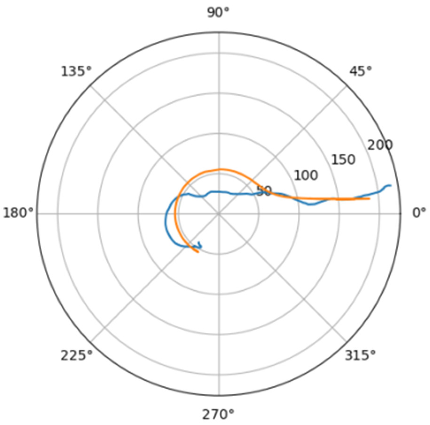
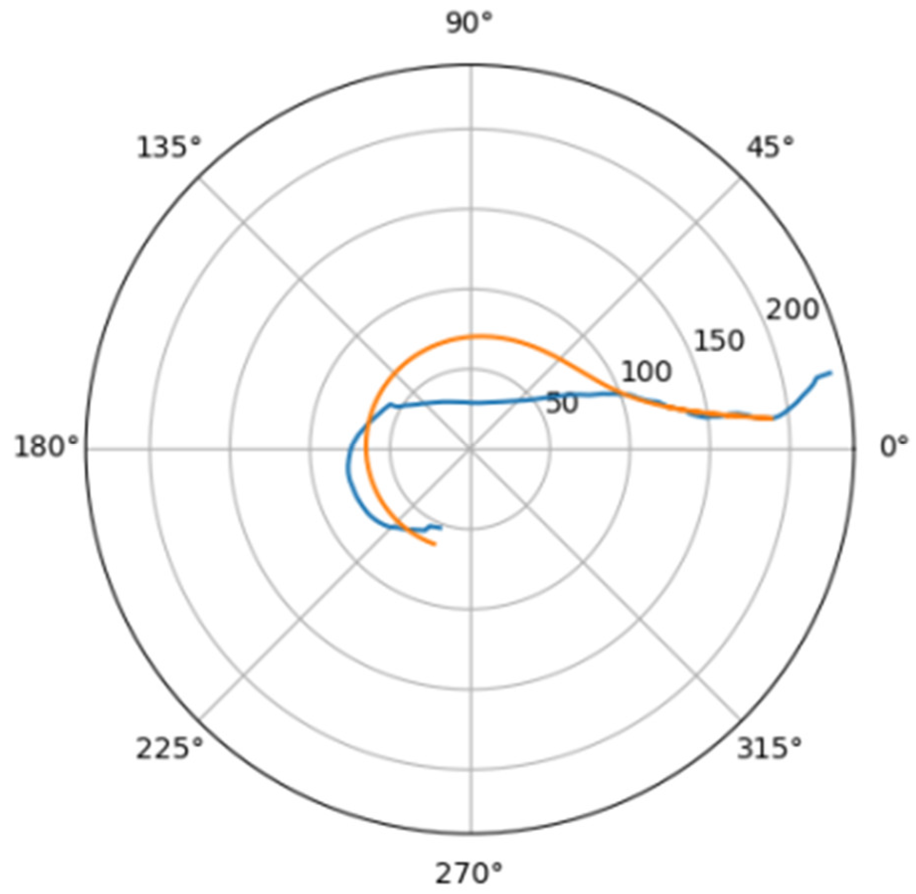
Approximating spirals for all central lines were constructed using an identical algorithm. The results obtained are shown in

Table 2. Comparison of the geometric characteristics of the approximation of the central line of the aorta.

Name	a	Power	bias	mae	${\mathit{R}}^2$	loc	feature_1	feature_2
are_s	2.896	7.893	−16.042	14.877	0.885	down	8.541	1.131
ino_s	4.008	5.256	−3.502	22.912	0.798	down	−3.933	9.622
ino_d	3.894	5.215	1.000	23.025	0.779	down	−8.834	9.775
she_a	3.125	6.702	0.993	15.979	0.894	down	−8.471	2.855
are_d	2.579	9.392	1.000	14.694	0.881	down	−8.522	0.384
bor_a	2.703	8.728	−131.587	14.359	0.925	down	124.059	−0.879
mal_a	3.009	7.190	1.000	13.648	0.892	down	−8.493	0.580
pav_a	0.426	17.357	1.000	18.678	0.810	down	−8.627	−0.195
mir_s	2.509	11.196	1.000	8.989	0.973	norm	−8.566	−5.461
bar_a	2.276	12.468	3.263	7.553	0.968	norm	−10.852	−7.325
zag_a	2.626	9.523	1.000	8.622	0.973	norm	−8.543	−4.959
mir_d	2.470	11.583	7.610	9.403	0.971	norm	−15.179	−5.227
gor_d	2.097	17.613	1.000	10.575	0.951	norm	−8.654	−7.230
poz_a	2.735	9.002	0.931	14.640	0.908	up	−8.447	0.539
hom_a	2.790	8.040	1.270	18.492	0.806	up	−8.760	4.365
lar_s	2.441	11.655	1.034	17.337	0.908	up	−8.580	1.574
lar_d	2.475	10.675	1.000	15.498	0.918	up	−8.538	0.452

$\left(\mathrm{a},\mathrm{power},\mathrm{bias}\right)$—parameters of the approximating hyperbolic spiral for the projection of the central line from expression (11), mae—the value of the standard deviation of the approximating curve from the projection of the central line, ${\mathrm{R}}^2$—coefficient of determination for a specific approximation, feature_1, feature_2—derived parameters, obtained from $\left(\mathrm{a},\mathrm{power},\mathrm{bias},{\mathrm{R}}^2,\mathrm{mae}\right)$ by PCA method.

.

As can be seen from the table, the value of the coefficient of determination $R^2$ for aortas without noticeable remodeling is higher, and the value of the standard deviation of the approximation mae is lower than for aortas with pathological disorders of the vascular bed. For normal aortas, the coefficient of determination exceeds 0.95, which indicates high approximation accuracy. For aortas with severe pathology of the vascular bed, the coefficient of determination exceeds 0.77, which indicates the significance of the chosen approximation method.

In Figure 6 was depicted approximation for normal aorta denoted as mir_s in Table 2. Other approximations are depicted on Figure 7, Figure 8, Figure 9, Figure 10, Figure 11, Figure 12, Figure 13, Figure 14, Figure 15, Figure 16, Figure 17, Figure 18, Figure 19, Figure 20, Figure 21 and Figure 22 The notations and lines color are the same, as on Figure 6.

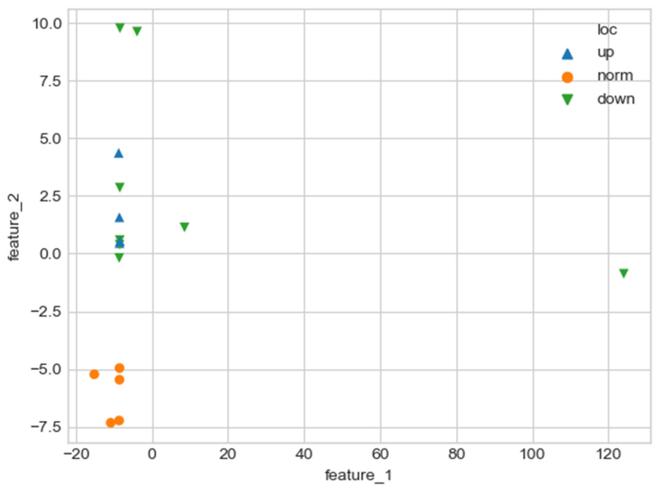
The values of the derived quantitative features feature_1 and feature_2 make it possible to unambiguously separate aortas without a noticeable pathological disorder and aortas with a violation of the geometry of the vascular bed (Figure 23).

The values of quantitative features (feature_1, feature_2), which were calculated by approximating the central line of the aortic flow channel with a hyperbolic spiral, make it possible to clearly separate the aorta without pronounced pathological remodeling and the aorta with pathological disturbance of the vascular bed. However, the obtained parameters do not allow one to reliably divide aortas according to the type of pathological remodeling (lesion in the proximal or distal sections).

As one can see, there is one obvious outlier on a plot from Figure 23. It is caused by a severely damaged aortic duct in the distal regions. As a result, the proposed algorithm can’t properly handle such altered geometry and issues biased values for features.

With a pathological violation of the geometry of the flow channel of the aorta, an area is formed in the local section of the channel, the radius of which significantly exceeds the radius of the same section in the norm. As follows from relations (2.1), for the volume of the swirling flow that fills this additional “pathological” region, at constant values of $C_0$ and ${\Gamma }_0$ the radial and azimuthal velocity components will be higher than in the normal case. An increase in the total linear velocity vector in the presence of severe pathological remodeling of the aortic duct was experimentally confirmed. However, if we assume that the parameters $C_0$ and ${\Gamma }_0$ for a pathological case normally coincide, the increase in the total vector of blood flow velocity in pathology will exceed the experimentally observed changes. Therefore, the value of ${\Gamma }_0$ in case of a pathological violation of the geometry of the flow channel will exceed the normal values to compensate for the increase in the radial size of the area with the aneurysm. The value of $C_0$ with pathology will increase slightly. This will lead to an insignificant increase in the radial and longitudinal departure velocity, which will cause an increase in the energy spent to maintain the evolution of the swirling flow. However, at the same time, an increase in the value of $C_0$ leads to a decrease in the viscous radius of the swirling flow (the region in which the influence of viscosity is strong). This will inevitably lead to a decrease in the energy spent on maintaining the twist. As a result, in case of a pathological violation of the geometry of the flow channel, we will get a small increase in the energy spent on maintaining the swirling blood flow; however, this value lies within the limits that approximately correspond to indirect observations.

4. Discussion

The geometric configuration of the aorta undergoes significant changes in various pathological conditions, such as hypertension, atherosclerosis, some infectious diseases, etc. At the same time, it is difficult to determine the stage at which changes in the geometry of the aortic flow channel are still compensatory in nature, and at which they are a manifestation of decompensation. There is no formal approach to the analysis of the geometric configuration of the aorta because the fields of force impact on the aortic wall, both in normal conditions and in the development of pathology, have not been sufficiently studied. The only source of force can be the flow of blood in the lumen of the aorta. However, there is still a discussion about the structure of this flow. Previously published papers have argued that the swirling flow pattern is of fundamental importance for adequate unseparated blood flow along the aorta. The shape of the lumen (longitudinal-radial size and distribution of elasticity along the aorta) corresponds with high accuracy to the directions of streamlines of the swirling flow described earlier using quasi-stationary equations (2.2). In the present study, an analysis of the spatial geometric configuration of the aorta in normal conditions and in lesions of predominantly proximal or distal sections was carried out. This analysis showed that the factors of the flow structure ($C_0$ and ${\Gamma }_0$) and the parameters of approximation of the projection of the aorta on the frontal plane of the human body by a hyperbolic spiral together make it possible to separate these states according to a formal feature.

As a result, new quantitative parameters characterizing the degree of pathological remodeling of the aortic duct and a method for their calculation were proposed. This method is based on a complex analysis of the geometry of the aortic flow channel. This analysis makes it possible to determine the hydrodynamic parameters of the swirling blood flow inside the aortic flow channel, the geometric correspondence of the shape of the flow channel to the direction of the swirling flow streamlines, and to formalize the geometry of the flow channel itself.

The field of shear stresses arising on the channel walls in a swirling flow regime differs significantly from the stresses arising in a fluid flow in laminar or turbulent regimes. Therefore, to analyze the impact of the flow on the walls of blood vessels, it is necessary to consider the twisted structure of the flow and to analyze the shape of the aorta parameters characterizing the degree of this twist—$C_0$ and ${\Gamma }_0$. The shape of the aorta is also determined by the nature of the swirling blood flow, so the channel geometry was approximated to a hyperbolic spiral. Only in a channel whose shape corresponds to a hyperbolic spiral is it possible to preserve the potentiality of the flow.

In this work, we used the geometric characteristics of the canal associated with the swirling blood flow in the canal lumen ($C_0$ and ${\Gamma }_0$), which made it possible to divide the aortas into 2 groups: the first group included normal aortas and aortas with pathology localized in the distal sections, and the second group included aorta with localization of pathology in the proximal sections. The construction of the central line and the approximation of this line to a hyperbolic spiral made it possible to further divide the aorta into 2 groups—the first included normal aorta, the second—aorta with lesions in the proximal and distal sections. At the same time, the error of the results does not exceed the threshold value adopted in experimental medicine (5%). The registered shifts in the values of the given parameters may reflect the type and severity of the pathology and may be considered predictors of critical conditions leading to the formation of aneurysms, dissections, and ruptures of the aortic wall.

5. Conclusions

New quantitative parameters were obtained, reflecting the degree of pathological remodeling of the aortic duct, as well a method for their calculation. These parameters can be useful for analyzing the mechanisms of aortic remodeling, determining the limits of compensatory changes in its geometry, and assessing the risks of decompensation leading to the formation of an aneurysm, dissection, or rupture of the aortic wall.